Non-Proportionality Indices and Error Constraint in Modal Analysis of Viscously Damped Linear Structures
Abstract
Featured Application
Abstract
1. Introduction
2. Materials and Methods
2.1. Proportional and Non-Proportional Damping
2.2. Indices to Measure Damping Non-Proportionality
- Nair and Singh (1986), INS1 [38].
2.3. Numerical Study
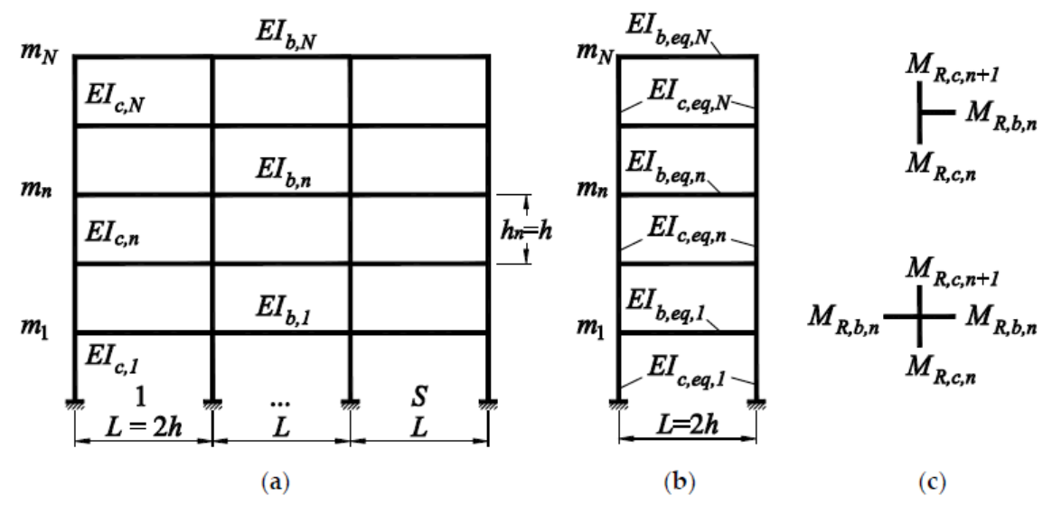
2.3.1. Systems Analyzed
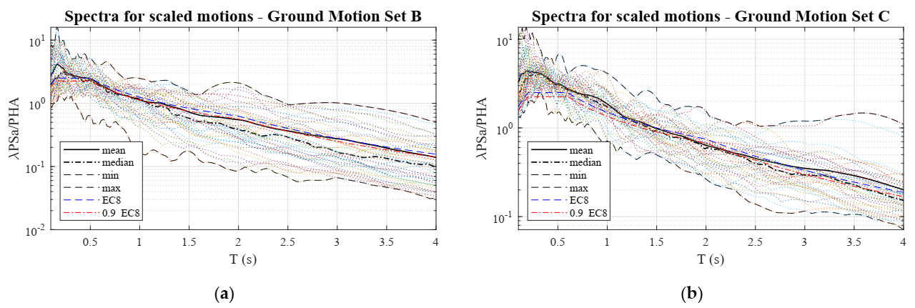
2.3.2. Ground Motions
2.3.3. Cases Examined
- Shear-type systems: B0-∞, B3-∞, B5-∞, C0-∞, C3-∞, C5-∞.
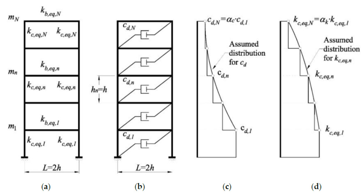
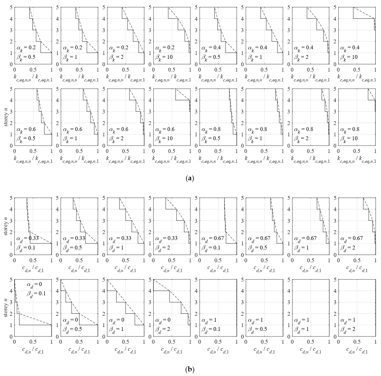
- Frame-type systems: B3-0.1, B3-0.5, B3-1, B3-2, B3-10, B0-1, B5-1, C3-1.
2.3.4. Procedures and Response Variables
- (1)
- Time-History (TH): the complete response ,, (relative displacement, relative velocity, and absolute acceleration, respectively) of the system defined by nsm, nsk and nsc (non-classically damped system) to each scaled register r in the GMS is calculated by the central difference step-by-step method [14]. The corresponding restoring forces and damping forces are obtained as and , respectively. Other variables are derived from these. The peak response for each variable and story is preserved.
- (2)
- Time-history modal analysis (THMA): the complete response , of the system defined by nsm, nsk and nscapprox (approximate classically damped system) to each scaled register r in the GMS, are calculated adding the responses obtained for each mode at each instant by the central difference step-by-step method. As in the previous procedure, restoring forces and damping forces are obtained as and , respectively; the forces obtained for every time-step are not in equilibrium, because is calculated using nsc whereas and are calculated using nscapprox, as is usual in design applications. Peak responses for every variable and story are preserved. THMA avoids the inaccuracies involved in the use of approximate modal combination rules, therefore only the first type of error discussed in Section 2.1 (due to neglected off-diagonal terms of the modal damping matrix) is present; this procedure is identified by subscript ‘1’.
- (3)
- Response spectrum analysis (RSA-SRSS and RSA-CQC): for every mode j of system ns defined by nsm, nsk and nscapprox (approximate classically damped system), and for every register r in the GMS, the modal peak relative displacement , modal peak relative velocity , and modal peak absolute acceleration , are found using the piecewise step-by-step method [43]. These vectors contain the peak values for every story at mode j, for example , etc. The modal peak values of restoring forces (= ) and damping forces (= ) are found. The modal peak values of other variables are derived from these. The peak response for every variable and story is obtained applying the SRSS rule (RSA-SRSS), identified with subscript ‘2’, or CQC rule (RSA-CQC), identified with subscript ‘3’. This option corresponds closely with the Response Spectrum Procedure defined in Chapter 18 of ASCE-SEI 7/16 [8], except that here it is applied only to linear systems. The SRSS [19] and CQC [20,21] rules are defined hereby for completeness:
2.3.5. Measure of Response Errors
3. Results
4. Discussion
4.1. Error Results for THMA (Error 1)
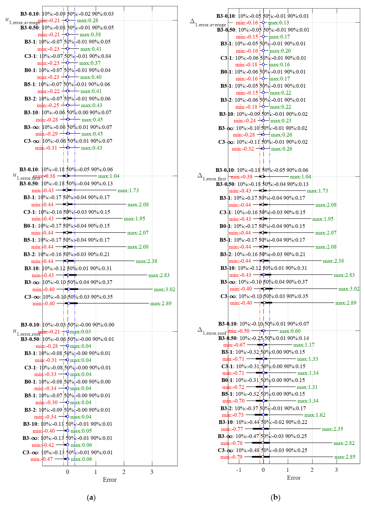
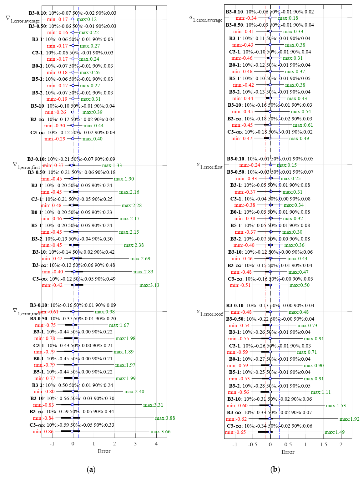
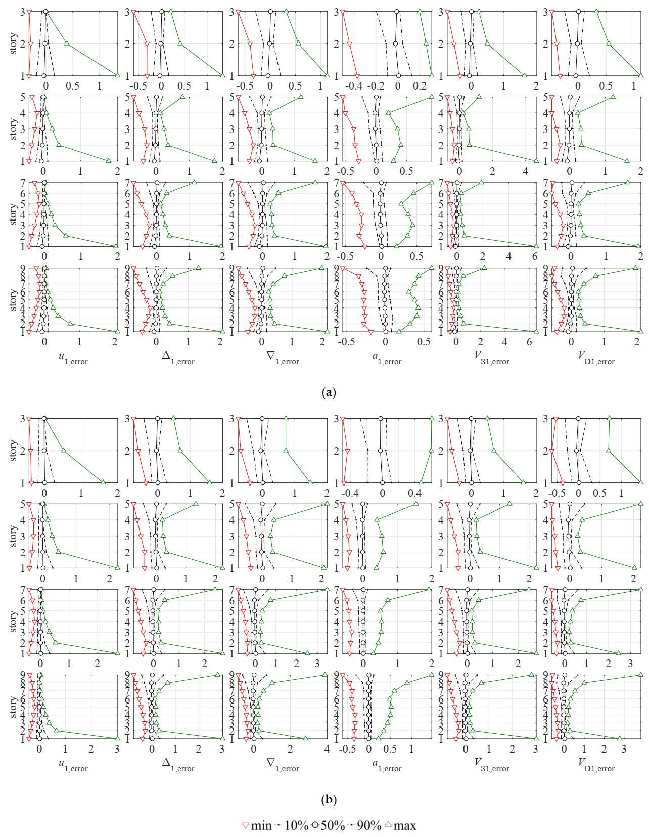
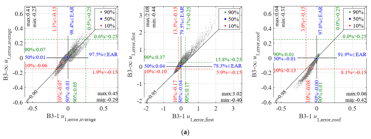
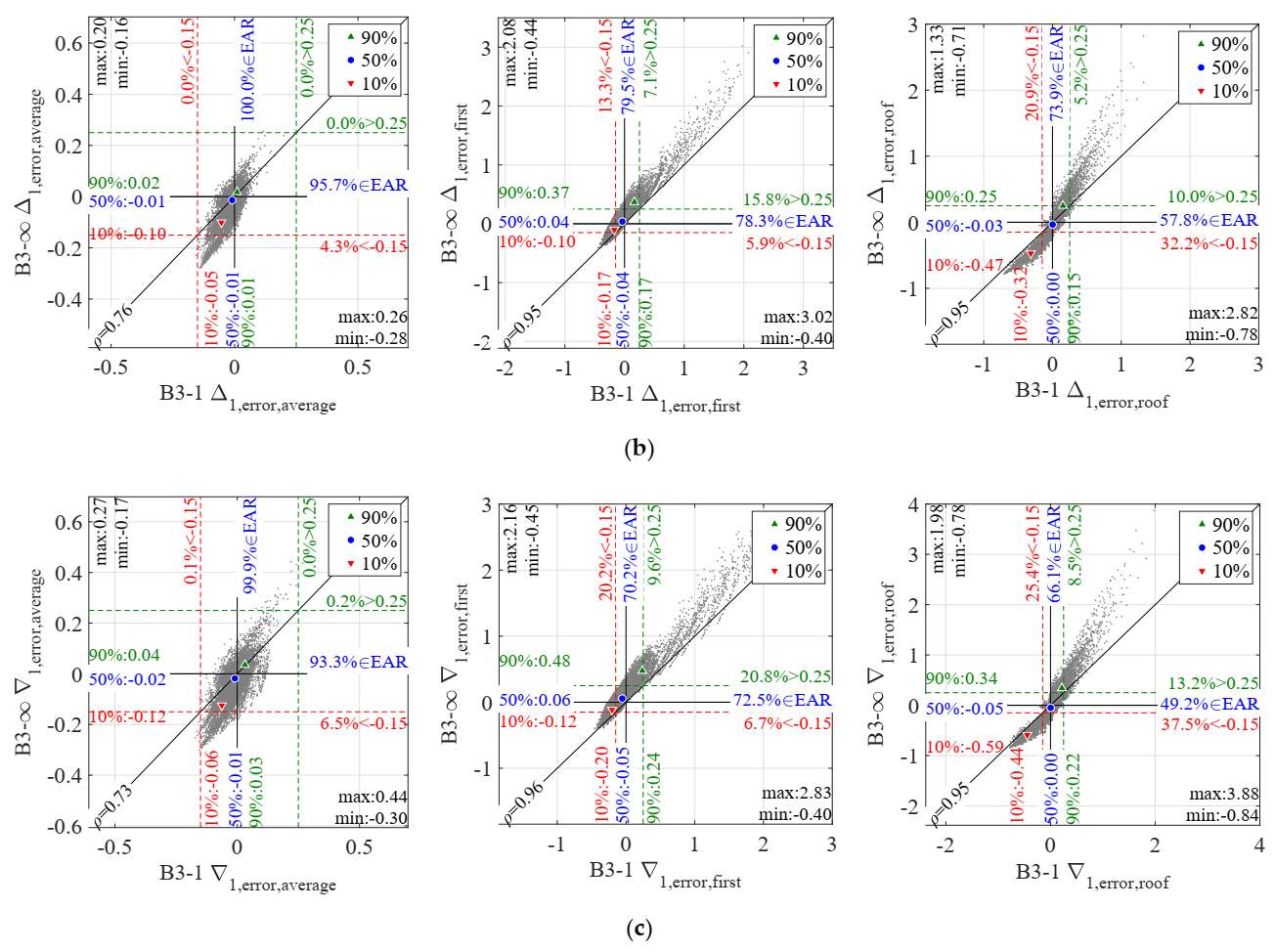
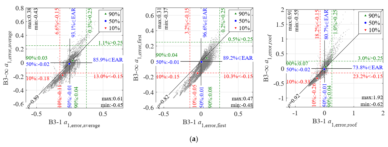
- As shown in Figure 3 and Figure A3, Figure A4 and Figure A5, Table 2 and Table 3, the median x50 for all cases, variables and stories is very close to 0, and the percentiles x10 and x90 are approximately contained within the indicative EAR [0.15; +0.25] except at roof, where a tendency for under-prediction (x10 below 0.15) exists for all variables except u1,error,roof; for this variable the prediction is excellent, as expected from the fact that the roof displacement is the key variable in the modal method. Indeed, the relative velocity error v1,error,roof is also very small. However, this is not the case for a1,error,roof.
- In general, the dispersion for all variables (except u1 and v1) is smaller in central stories of the frame and increases at the top and bottom (Figure 3); the 3-story frame is an exception where x90 and max generally diminish at the top.
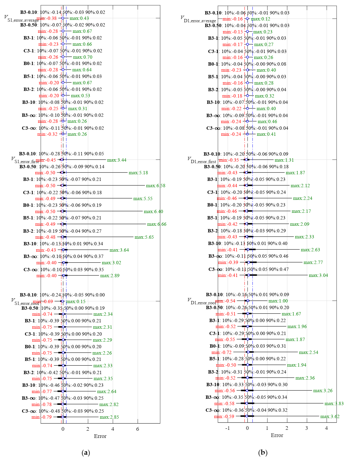
- When the average across stories is examined (Figure A3, Figure A4 and Figure A5, Table 2 and Table 3), THMA offers a reasonable accuracy for all variables analyzed. The behavior is particularly good for Δ1,error,average, and for the static variables VS1,error,average and VD1,error,average. The worst behavior is observed for a1,error,average, with a tendency to under-prediction. In all cases, a reduced number of extreme values give errors well outside the indicative EAR. Extreme errors are more pronounced for shear-type systems except for VS1,error,average.
- When the first story error is examined, larger extreme errors are found, particularly for the maximum in all variables except a1,error,first. The over-conservative error reaches particularly high values (up to 6.66 for B5-1) for VS1,error,first. For other variables, approximately up to 3. Remarkable minimum extreme errors are also found.
- When the roof error is examined (except for variable u1,error,roof), results present a larger dispersion, and in general are more un-conservative than those of the average or first story. The minimum errors are more extreme for this story, and in fact x10 for most cases generally falls below 0.15; large maximum errors are also found, in some variables (a1,error,roof, VD1,error,roof) even above the corresponding maxima of the first story error.
- Regarding the influence of inherent damping, comparison of results between B0-1, B3-1 and B5-1 in Figure A3, Figure A4 and Figure A5, are virtually identical for all variables and stories, showing that this parameter does not influence the error; because inherent damping has been modeled as modal damping this result was expected.
- Regarding the influence of ground type, comparison of error results between B3-1 vs. C3-1, and B3-∞ vs. C3-∞ show that this parameter exerts a very mild influence on the error. The influence is only apparent in the extreme errors, particularly in the maximum error, but x10, x50 and x90 are virtually unaffected. This influence is due to the mean spectrum peculiarities of each set.
- Shear-type and frame-type systems render similar median errors, but with a larger dispersion in the former. As is clear in Figure A3, Figure A4 and Figure A5, the median value x50 is quite stable across cases, but the min and x10 decrease for shear-type systems, whereas the max and x90 increase. These differences are also clear in Figure 3. Therefore, the maximum and minimum errors expected are those corresponding to shear-type systems, except for VS1,error,first, where frame-type systems present more extreme max and min errors. It is worth noticing that Δ1,error and VS1,error are equal in shear-type systems, whereas they differ in frame-type systems.
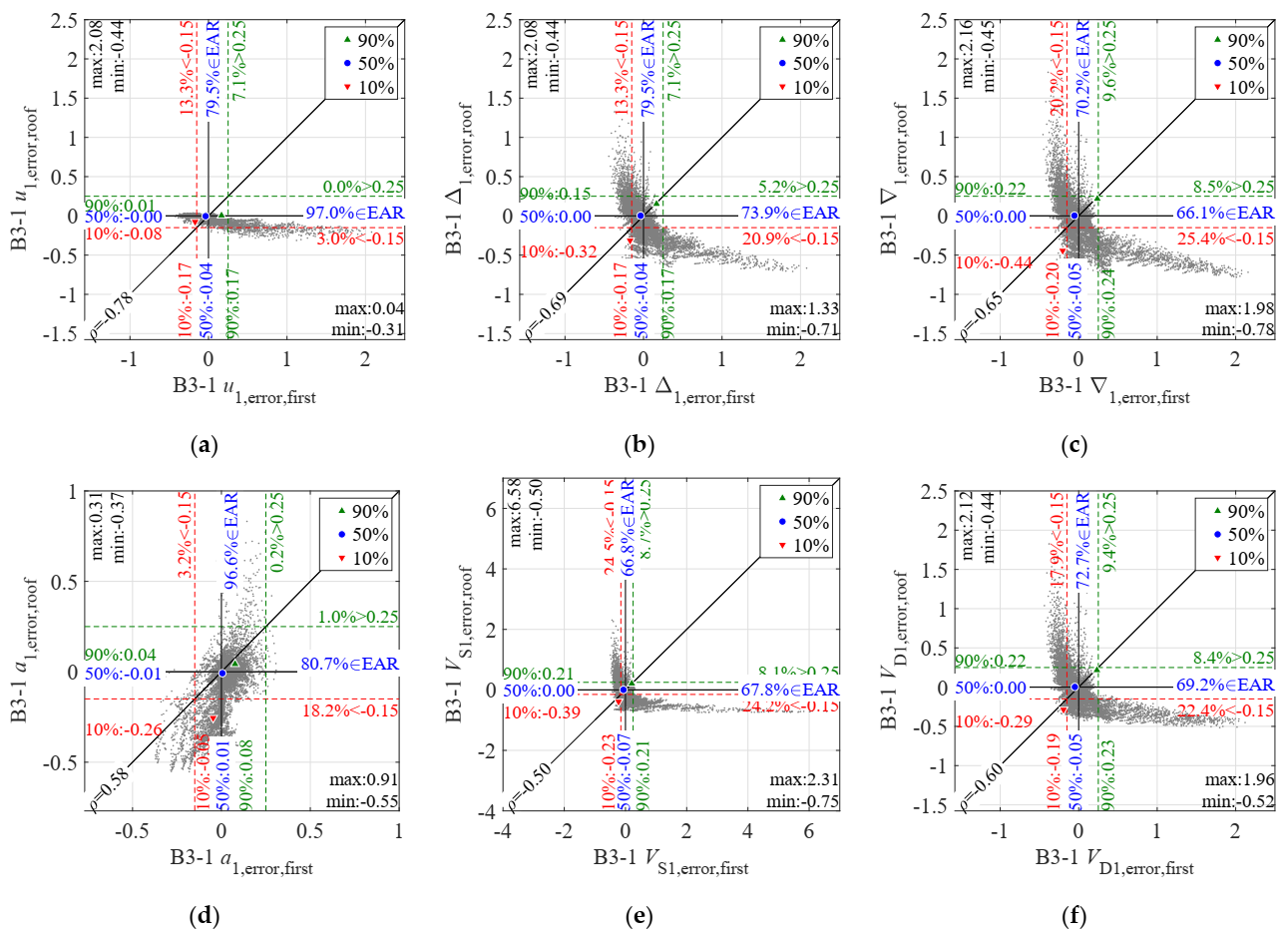
- It is concluded that although average errors across the system height tend to be centered around 0, individual stories (particularly first story and roof) will present large errors; the tendency of average errors to be small is due to the negative correlation between errors at the first story and roof; this trend is clear in Figure 6, where a scatter plot of first story THMA error (error 1) versus THMA roof error for all variables is presented; the plot shows that positive errors at roof are generally accompanied by negative errors at first story, and conversely; due to the different sign of top and bottom error, the average across stories is small. This stands for all variables except displacement u1 (due to the small error at roof) and acceleration a1.
4.2. Error Results for RSA-SRSS (Error 2) and RSA-CQC (Error 3)
- The general trends are very similar between both combination rules and THMA, except for a larger dispersion in most of the variables, and substantial differences in a.
- Considering the average across stories, the median x50 is close to 0 and the dispersion (measured by x10 and x90) is moderate, except for ∇, a, and VS. The over-conservative error (max) is considerably smaller for all variables (except u and v) when the RSA-CQC method (error 3) is used.
- Considering the first story error, the median x50 is negative with both methods and for all variables, indicating that both RSA-SRSS and RSA-CQC tend to under-predict results at this story. However, RSA-SRSS (error 2) renders slightly more un-conservative results, therefore more extreme min values. However, larger over-conservative results for x90 and max are obtained with RSA-CQC (error 3).
- Considering the roof error, both methods tend to conservative (>0) median x50 results. More extreme un-conservative results min and x10 are obtained with RSA-CQC (error 3), but more extreme conservative results x90 and max are obtained with RSA-SRSS (error 2).
- The influence of inherent damping, type of system (shear-type or frame-type) and ground type follows the same trends as in THMA.
- As a conclusion, RSA-SRSS and RSA-CQC methods are expected to render reasonable average results across stories but generally produce un-conservative results for first story and over-conservative results for the roof. Dispersion (measured as x90-x10) is larger for RSA-SRSS. Overall, both methods are very similar for u and v. RSA-CQC offers better results for all other variables.
4.3. Identification of Significant Parameters
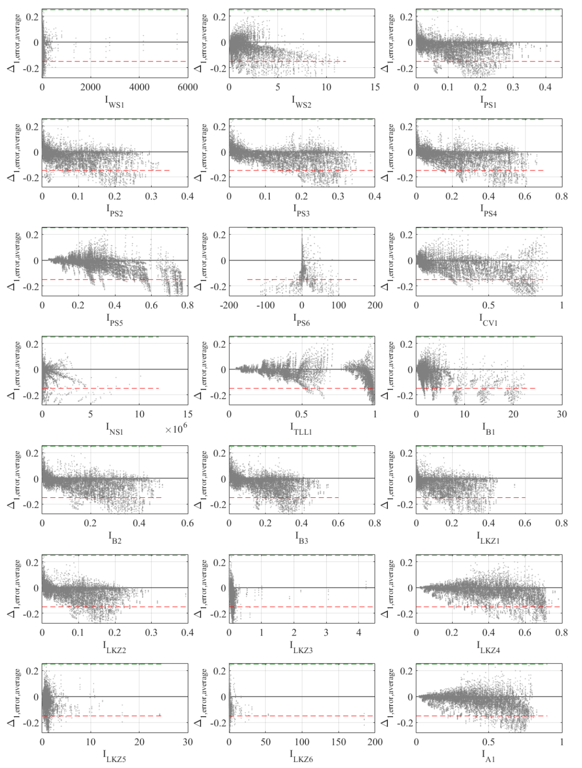
4.4. Correlation of Error Results with Existing Non-Proportionality Indices
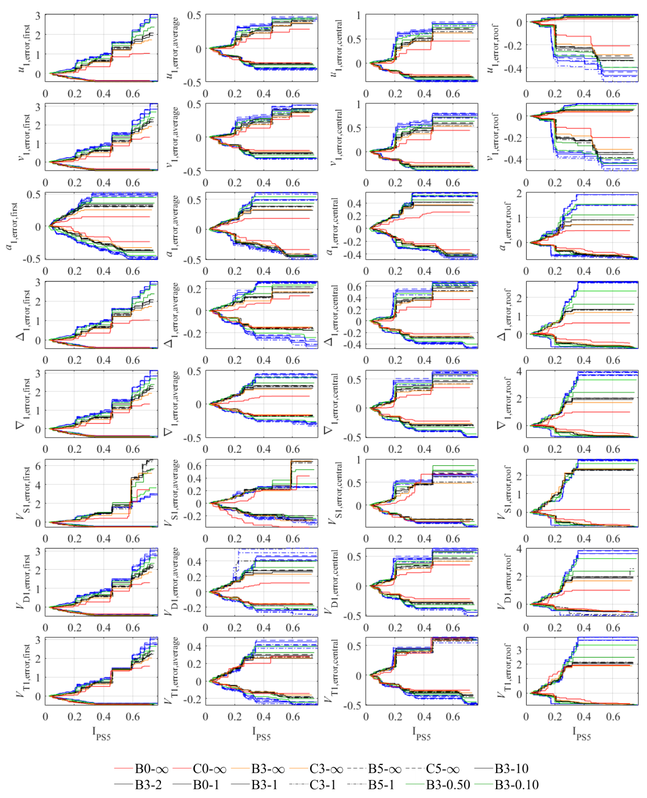
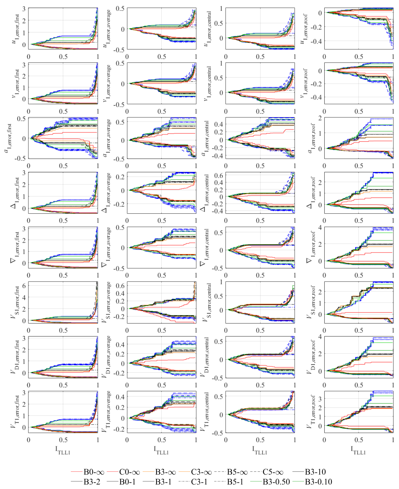
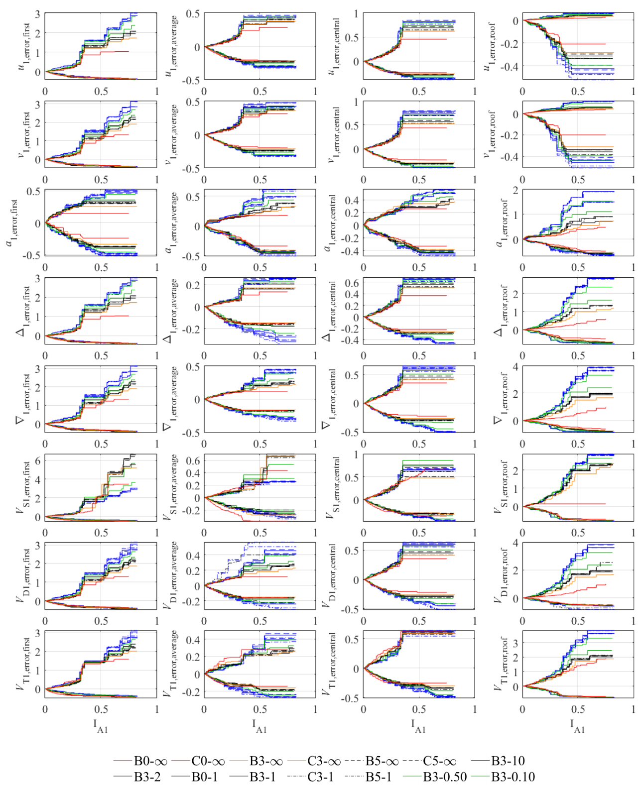
- The relationship between THMA error for a certain variable at a certain story and the same NPI follows similar trends for all cases in the study, regardless of the index considered. The curves corresponding to different cases are, in all cases, closely squeezed together.
- The differences between cases are mostly due to model type: shear-type cases (B0-∞, B3-∞, B5-∞, C0-∞, C3-∞, C5-∞) present more extreme errors and generally correspond to the outermost curve; contrariwise, the extreme case of frame-type system (B3-0.10) presents the innermost curve of the collection. The only exception is VS1,average where for all indices the min un-conservative error corresponds to B3-0.10.
- Inherent damping and ground type exert a very mild influence; for the same λ, the curves corresponding to different inherent damping ratios are practically identical, as are the curves corresponding to different ground types. An exception happens at VD1,error,average with indices IPS5 and IA1, where the 0% case presents a steeper increase of conservative error. This trend is not detected in index ITLL1.
- The absolute value of un-conservative error is, in general, much smaller than the conservative error. However, for some specific variables and stories, similar orders of magnitude are obtained for both extreme errors.
5. Conclusions
- (1)
- The error in THMA is only mildly dependent on inherent damping and ground type; its median value is close to 0 and generally 80% of the results are within a range of [0.15; +0.25]; conservative (max) errors are larger than un-conservative (min) errors. Large error dispersion occurs at the bottom and top of the frames, with a negative correlation between both stories. Shear-type systems present, in general, larger extreme errors than frame-type systems.
- (2)
- RSA present similar trends to THMA, but with larger dispersion and a tendency to un-conservative errors at first story and over-conservative errors at the roof. RSA-CQC offers a smaller dispersion than RSA-SRSS.
- (3)
- To keep the error under a certain threshold in THMA and RSA, simple criteria based on frame and damping system properties cannot be proposed from the data available, as parameters that are significant for the response averaged through stories, central story, first story and roof are generally different. Moreover, values of parameters that reduce the response error in one story might trigger a large error in another.
- (4)
- A correlation of the max and min error in THMA and RSA with four existing non-proportionality indices has been empirically proved and can be used as an alternative method to keep the error under control, especially for THMA. Tabulated data for different error thresholds are provided.
Supplementary Materials
Author Contributions
Funding
Institutional Review Board Statement
Informed Consent Statement
Data Availability Statement
Conflicts of Interest
Appendix A. Description of Non-Proportionality Indices
Appendix A.1. Warburton and Soni
Appendix A.2. Prater and Singh
Appendix A.3. Nair and Singh
Appendix A.4. Claret and Venancio-Filho
Appendix A.5. Tong, Liang and Lee
Appendix A.6. Bhaskar
Appendix A.7. Liu, Kujath and Zheng
Appendix A.8. Prells and Friswell
Appendix A.9. Adhikari
Appendix B. Determination of Range for Parameter λ
- (1)
- MR,c,n = MR,c,n+1 leading to the condition MR,c,n ≥ 1.3MR,b,n;
- (2)
- MR,c,n >> MR,c,n+1 leading to the condition MR,c,n ≥ 2.6MR,b,n.
| S | Scenario #1 MR,c,n = MR,c,n+1 ⇒ MR,c,n ≥ 1.3MR,b,n | Scenario #2 MR,c,n >> MR,c,n+1 ⇒ MR,c,n ≥ 2.6MR,b,n | ||||
|---|---|---|---|---|---|---|
| μ | σ | cv = σ/μ | μ | σ | cv = σ/μ | |
| 1 | 0.90 | 0.11 | 0.12 | 0.35 | 0.05 | 0.14 |
| 2 | 1.20 | 0.14 | 0.12 | 0.47 | 0.07 | 0.15 |
| 3 | 1.35 | 0.16 | 0.12 | 0.52 | 0.07 | 0.13 |
| 4 | 1.44 | 0.17 | 0.12 | 0.56 | 0.08 | 0.14 |
| 10 | 1.64 | 0.19 | 0.12 | 0.64 | 0.09 | 0.14 |
Appendix C. Ground Motion Selection
| Name | Station | Date | Fault | Mw | Epic. Dist. (km) | PHAX (g) | PHAY (g) | Prescaleλx (1) | Prescaleλy (1) |
|---|---|---|---|---|---|---|---|---|---|
| Friuli (aftershock) | Forgaria-Cornio | 15.09.1976 | thrust | 6 | 17 | 0.264 | 0.218 | 2.861 | 2.085 |
| Friuli (aftershock) | Forgaria-Cornio | 15.09.1976 | thrust | 6 | 17 | 0.346 | 0.336 | 2.230 | 1.537 |
| Montenegro | Bar-SkupstinaOpstine | 15.04.1979 | thrust | 6.9 | 16 | 0.375 | 0.363 | 0.909 | 0.720 |
| Montenegro (aftershock) | Tivat-Aerodrom | 24.05.1979 | thrust | 6.2 | 21 | 0.166 | 0.133 | 2.481 | 2.198 |
| Montenegro (aftershock) | Petrovac-Hotel Oliva | 15.05.1979 | oblique | 5.8 | 24 | 0.099 | 0.089 | 1.451 | 1.211 |
| Campano Lucano | Calitri | 23.11.1980 | normal | 6.9 | 16 | 0.156 | 0.176 | 0.707 | 0.768 |
| Kalamata | Kalamata-Prefecture | 13.09.1986 | normal | 5.9 | 10 | 0.215 | 0.297 | 0.819 | 0.982 |
| Kyllini | Zakynthos-OTE Building | 16.10.1988 | strike slip | 5.9 | 14 | 0.151 | 0.146 | 0.685 | 1.367 |
| Erzincan | Erzincan-Meteorologij | 13.03.1992 | strike slip | 6.6 | 13 | 0.389 | 0.513 | 0.765 | 1.164 |
| Tithorea | Aigio-OTE Building | 18.11.1992 | normal | 5.9 | 25 | 0.038 | 0.028 | 0.807 | 1.932 |
| Umbria Marche | Gubbio-Piana | 26.09.1997 | normal | 6 | 38 | 0.091 | 0.097 | 0.838 | 0.760 |
| Potenza | Brienza | 05.05.1990 | strike slip | 5.8 | 28 | 0.096 | 0.080 | 2.208 | 1.534 |
| AnoLlosia | Athens 2 (Chalandri District) | 07.09.1999 | normal | 6 | 20 | 0.110 | 0.161 | 2.121 | 2.411 |
| Griva | Edessa-Prefecture | 21.12.1990 | normal | 6.1 | 36 | 0.101 | 0.096 | 0.899 | 1.100 |
| South Aegean | Heraklio-Technical University | 23.05.1994 | oblique | 6.1 | 45 | 0.061 | 0.041 | 1.212 | 0.814 |
| Strofades | Zakynthos-OTE Building | 18.11.1997 | oblique | 6.6 | 38 | 0.131 | 0.116 | 1.152 | 1.542 |
| Kozani | Kastoria-OTE Building | 13.05.1995 | normal | 6.5 | 50 | 0.019 | 0.020 | 1.024 | 1.272 |
| Aigion | Patra-San Dimitrios Church | 15.06.1995 | normal | 6.5 | 43 | 0.084 | 0.093 | 0.713 | 0.976 |
| Duzce 1 | LDEO Station No C1058 BV | 12.11.1999 | oblique | 7.2 | 11 | 0.111 | 0.073 | 1.257 | 1.044 |
| Firuzabad | Firoozabad | 20.06.1994 | strike slip | 5.9 | 22 | 0.250 | 0.278 | 3.366 | 3.481 |
| Name | Station | Date | Fault | Mw | Epic. Dist. (km) | PHAX (g) | PHAY (g) | Prescaleλx (1) | Prescaleλy (1) |
|---|---|---|---|---|---|---|---|---|---|
| Ionian | Lefkada-OTE Building | 04.11.1973 | thrust | 5.8 | 15 | 0.525 | 0.255 | 1.576 | 1.604 |
| Friuli | Buia | 15.09.1976 | thrust | 6 | 11 | 0.083 | 0.090 | 1.472 | 1.858 |
| Volvi | Thessaloniki-City Hotel | 20.06.1978 | normal | 6.2 | 29 | 0.139 | 0.146 | 1.612 | 1.741 |
| Alkion | Korinthos-OTE Building | 24.02.1981 | normal | 6.6 | 20 | 0.230 | 0.299 | 1.394 | 1.900 |
| Alkion | Korinthos-OTE Building | 25.02.1981 | normal | 6.3 | 25 | 0.117 | 0.120 | 1.336 | 1.161 |
| Spitak | Gukasian | 07.12.1988 | thrust | 6.7 | 36 | 0.183 | 0.183 | 1.708 | 1.427 |
| Spitak (aftershock) | Gukasian | 07.12.1988 | thrust | 5.8 | 36 | 0.147 | 0.103 | 1.896 | 1.987 |
| Umbria Marche | Matelica | 26.09.1997 | normal | 5.7 | 27 | 0.046 | 0.049 | 2.235 | 2.241 |
| Umbria Marche | Matelica | 26.09.1997 | normal | 6 | 27 | 0.117 | 0.109 | 2.409 | 2.088 |
| Umbria Marche (aftershock) | Colfiorito | 14.10.1997 | normal | 5.6 | 13 | 0.092 | 0.068 | 1.705 | 1.450 |
| Sicilia-Orientale | Catania-Piana | 13.12.1990 | strike slip | 5.6 | 24 | 0.253 | 0.182 | 4.148 | 3.449 |
| Izmit | Yarimca-Petkim | 17.08.1999 | strike slip | 7.6 | 20 | 0.296 | 0.244 | 1.178 | 1.107 |
| Duzce | Bolu-Bayindirlik | 12.11.1999 | oblique | 7.2 | 39 | 0.745 | 0.800 | 1.803 | 1.864 |
| Ano Liosia | Athens-Neo Psihiko | 07.09.1999 | normal | 6 | 19 | 0.083 | 0.101 | 2.122 | 1.999 |
| Cubuklu | Muradiye-Meteoroloji | 20.04.1998 | oblique | 5.5 | 34 | 0.042 | 0.045 | 1.181 | 0.902 |
| Filippias | Lefkada-Hospital | 16.06.1990 | thrust | 5.5 | 44 | 0.020 | 0.031 | 1.121 | 1.197 |
| Kyllini | Pyrgos-Agriculture Bank | 16.10.1988 | strike slip | 5.9 | 49 | 0.025 | 0.030 | 1.357 | 1.847 |
| Duzce 3 (aftershock) | Duzce-Meteoroloji | 23.08.2000 | strike slip | 5.5 | 41 | 0.023 | 0.017 | 3.166 | 2.522 |
| Bovec | Gemona-Scugelars | 12.04.1998 | strike slip | 5.6 | 38 | 0.024 | 0.040 | 2.044 | 4.122 |
| Izmit (aftershock) | Yarimca-Petkim | 13.09.1999 | oblique | 5.8 | 27 | 0.088 | 0.092 | 1.742 | 1.745 |
Appendix D. Additional Plots
References
- Soong, T.; Dargush, G.F. Passive Energy Dissipation Systems in Structural Engineering, 1st ed.; Wiley: Hoboken, NJ, USA, 1997. [Google Scholar]
- Christopoulos, C.; Filiatrault, A. Principles of Passive Supplemental Damping and Seismic Isolation; Iuss Press: Pavia, Italy, 2006. [Google Scholar]
- Symans, M.D.; Charney, F.A.; Whittaker, A.S.; Constantinou, M.C.; Kircher, C.A.; Johnson, M.W.; McNamara, R.J. Energy dissipation systems for seismic applications: Current practice and recent developments. J. Struct. Eng. 2008, 134, 3–21. [Google Scholar] [CrossRef]
- Constantinou, M.C.; Symans, M.D. Experimental and Analytical Investigation of Seismic Response of Structures with Supplemental Fluid Viscous Dampers; National Center for Earthquake Engineering Research: Buffalo, NY, USA, 1992. [Google Scholar]
- Seleemah, A.A.; Constantinou, M.C. Investigation of Seismic Response of Buildings with Linear and Nonlinear Fluid Viscous Dampers; National Center for Earthquake Engineering Research: Buffalo, NY, USA, 1997. [Google Scholar]
- Caughey, T.K.; O’Kelly, M.E.J. Classical normal modes in damped linear dynamic systems. J. Appl. Mech. 1965, 32, 583–588. [Google Scholar] [CrossRef]
- Federal Emergency Management Agency. FEMA 273: NEHRP Guidelines for the Seismic Rehabilitation of Buildings; FEMA: Washington, DA, USA, 1997.
- American Society of Civil Engineers (ASCE), A.S.O.C. Minimum Design Loads and Associated Criteria for Buildings and Other Structures; American Society of Civil Engineers (ASCE): Reston, VA, USA, 2017. [Google Scholar] [CrossRef]
- Labbé, P. Outlines of the revision of the Eurocode 8, part 1-generic clauses. In Proceedings of the 16th European Conference on Earthquake Engineering, Thessaloniki, Greece, 18–21 June 2018. [Google Scholar]
- Foss, K.A. Coordinates which uncouple the equations of motion of damped linear dynamic systems. J. Appl. Mech. 1958, 25, 361–364. [Google Scholar] [CrossRef]
- Veletsos, A.S.; Ventura, C.E. Modal analysis of non-classically damped linear systems. Earthq. Eng. Struct. Dyn. 1986, 14, 217–243. [Google Scholar] [CrossRef]
- Hanson, R.D.; Soong, T.T. Seismic Design with Supplemental Energy Dissipation Devices; Earthquake Engineering Research Institute: Oakland, CA, USA, 2001. [Google Scholar]
- Ramirez, O.M.; Constantinou, M.C.; Kircher, C.A.; Whittaker, A.; Johnson, M.; Gomez, J.D.; Chrysostomou, C.Z. Development and Evaluation of Simplified Procedures of Analysis and Design for Structures with Passive Energy Dissipation Systems; Technical Report No. MCEER-00–0010, Revision 1; Multidisciplinary Center for Earthquake Engineering Research, University of Buffalo: Buffalo, NY, USA, 2001. [Google Scholar]
- Clough, R.W.; Penzien, J. Dynamics of Structures, 3rd ed.; Computers and Structures: Berkeley, CA, USA, 2013. [Google Scholar]
- Kasai, K.; Fu, Y.; Watanabe, A. Passive Control Systems for Seismic Damage Mitigation. J. Struct. Eng. 1998, 124, 501–512. [Google Scholar] [CrossRef]
- Guo, J.W.W.; Christopoulos, C. Performance Spectra Based Method for the Seismic Design of Structures equipped with Passive Supplemental Damping Systems. Earthq. Eng. Struct. Dyn. 2013, 42, 935–952. [Google Scholar] [CrossRef]
- Chopra, A.K. Dynamics of Structures: Theory and Applications to Earthquake Engineering, 3rd ed.; Pearson Prentice Hall: Hoboken, NJ, USA, 2007. [Google Scholar]
- Caughey, T.K. Classical normal modes in damped linear dynamic systems. J. Appl. Mech. 1960, 27, 269–271. [Google Scholar] [CrossRef]
- Goodman, L.E.; Rosenblueth, E.; Newmark, N.M. Aseismic Design of Elastic Structures Founded on Firm Ground; Civil Engineering Studies SRS-026; University of Illinois Engineering Experiment Station, College of Engineering, University of Illinois at Urbana-Champaign: Urbana, IL, USA, 1952. [Google Scholar]
- Der Kiureghian, A. On Response of Structures to Stationary Excitation; University of California, Earthquake Engineering Research Center: Berkeley, CA, USA, 1979. [Google Scholar]
- Der Kiureghian, A. A Response Spectrum Method for Random Vibrations; University of California, Earthquake Engineering Research Center: Berkeley, CA, USA, 1980. [Google Scholar]
- Falsone, G.; Muscolino, G. New real-value modal combination rules for non-classically damped structures. Earthq. Eng. Struct. Dyn. 2004, 33, 1187–1209. [Google Scholar] [CrossRef]
- De Domenico, D.; Falsone, G.; Ricciardi, G. Improved response-spectrum analysis of base-isolated buildings: A substructure-based response spectrum method. Eng. Struct. 2018, 162, 198–212. [Google Scholar] [CrossRef]
- De Domenico, D.; Ricciardi, G.; Takewaki, I. Design strategies of viscous dampers for seismic protection of building structures: A review. Soil Dyn. Earthq. Eng. 2019, 118, 144–165. [Google Scholar] [CrossRef]
- Conde, J. Seismic Response of Structures Equipped with Passive Energy Dissipation Systems Using Simplified Methods Based on Equivalent Effective Properties. Ph.D. Thesis, Universidad Politécnica de Madrid (UPM), Madrid, Spain, 2020. [Google Scholar] [CrossRef]
- Liang, Z.; Lee, G.C. Damping of Structures: Part 1-Theory of Complex Damping; National Center for Earthquake Engineering Research, University of Buffalo: Buffalo, NY, USA, 2001. [Google Scholar]
- Luo, D.Z. A graphic explanation of undamped and damped mode shapes and its application. J. Sound Vib. 1989, 135, 351–356. [Google Scholar] [CrossRef]
- Warburton, G.B.; Soni, S.R. Errors in response calculations for non-classically damped structures. Earthq. Eng. Struct. Dyn. 1977, 5, 365–376. [Google Scholar] [CrossRef]
- Prater, G., Jr.; Singh, R. Quantification of the extent of non-proportional viscous damping in discrete vibratory systems. J. Sound Vib. 1986, 104, 109–125. [Google Scholar] [CrossRef]
- Claret, A.M.; Venancio-Filho, F. A modal superposition pseudo-force method for dynamic analysis of structural systems with non-proportional damping. Earthq. Eng. Struct. Dyn. 1991, 20, 303–315. [Google Scholar] [CrossRef]
- Tong, M.; Liang, Z.; Lee, G.C. An index of damping non-proportionality for discrete vibrating systems. J. Sound Vib. 1994, 174, 37–55. [Google Scholar] [CrossRef]
- Bhaskar, A. Estimates of errors in the frequency response of non-classically damped systems. J. Sound Vib. 1995, 184, 59–72. [Google Scholar] [CrossRef]
- Bhaskar, A. Mode shapes during asynchronous motion and non-proportionality indices. J. Sound Vib. 1999, 224, 1–16. [Google Scholar] [CrossRef][Green Version]
- Liu, K.; Kujath, M.R.; Zheng, W. Quantification of non-proportionality of damping in discrete vibratory systems. Comput. Struct. 2000, 77, 557–570. [Google Scholar] [CrossRef]
- Liu, K.; Kujath, M.R.; Zheng, W. Evaluation of damping non-proportionality using identified modal information. Mech. Syst. Signal Process. 2001, 15, 227–242. [Google Scholar] [CrossRef]
- Prells, U.; Friswell, M.I. A measure of non-proportional damping. Mech. Syst. Signal Process. 2000, 14, 125–137. [Google Scholar] [CrossRef][Green Version]
- Adhikari, S. Optimal complex modes and an index of damping non-proportionality. Mech. Syst. Signal Process. 2004, 18, 1–27. [Google Scholar] [CrossRef]
- Nair, S.S.; Singh, R. Examination of the validity of proportional damping approximations with two further numerical indices. J. Sound Vib. 1986, 104, 348–350. [Google Scholar] [CrossRef]
- Conde, J.; Bernabeu, A. Influence of Maxwell Stiffness in Damage Control and Analysis of Structures with Added Viscous Dampers. Appl. Sci. 2021, 11, 3089. [Google Scholar] [CrossRef]
- Ambraseys, N.; Smit, P.; Douglas, J.; Margaris, B.; Sigbjörnsson, R.; Olafsson, S.; Suhadolc, P.; Costa, G. Internet site for European strong-motion data. Boll. Geofis. Teor. Appl. 2004, 45, 113–129. [Google Scholar]
- ESD, European Strong-Motion Database. Available online: http://www.isesd.hi.is/ESD_Local/frameset.htm (accessed on 9 February 2021).
- European Committee for Standardization. En-1998-1: 2004. Eurocode 8: Design of Structures for Earthquake Resistance. Part 1: General Rules, Seismic Actions and Rules for Buildings; CEN: Brussels, Belgium, 2004. [Google Scholar]
- Nigam, N.C.; Jennings, P.C. Calculation of response spectra from strong-motion earthquake records. Bull. Seismol. Soc. Am. 1969, 59, 909–922. [Google Scholar]
- Guyader, A.C.; Iwan, W.D. Determining equivalent linear parameters for use in a capacity spectrum method of analysis. J. Struct. Eng. 2006, 132, 59–67. [Google Scholar] [CrossRef]
- Nakashima, M.; Ogawa, K.; Inoue, K. Generic frame model for simulation of earthquake responses of steel moment frames. Earthq. Eng. Struct. Dyn. 2002, 31, 671–692. [Google Scholar] [CrossRef]

| Procedure | TH | THMA | RSA-SRSS (**) |
| Description. | Time history step-by-step analysis | Time history modal analysis | Response spectrum analysis |
| System ns definition (ns = 1 to 13312). | nsm, nsk, nsc | nsm, nsk, nscapprox | nsm, nsk, nscapprox |
| Analysis method. | Central difference applied to complete system. | Central difference applied to complete system. | Exact piecewise applied to each mode. |
| Solution type (for register r in case nc). | Complete solution. . | Complete solution. . | Peak modal solution (mode j). . |
| Total damping forces (for register r in case nc). | . | . | |
| Variables derived from solution (for register r in case nc). | , , | ||
| Peak solution (for register r in case nc and story s). | . Similar for other variables. | . Similar for other variables. | . Similar for other variables (**). |
| Error for register r in case nc and story s. | Does not apply | . Similar for other variables. | . Similar for other variables. |
| Significant stories considered. | Does not apply | First: . Central: . Roof: . Average: . Similar for other variables. | First: . Central: . Roof: . Average: . Similar for other variables. |
| Final error for system ns and case nc at story s. | Does not apply | , where s = first, central, average, roof.Similar for other variables. | , where s = first, central, average, roof.Similar for other variables |
| First Story | Average Across Stories | Roof | ||||||||||||||
|---|---|---|---|---|---|---|---|---|---|---|---|---|---|---|---|---|
| min | x10 | x50 | x90 | max | min | x10 | x50 | x90 | max | min | x10 | x50 | x90 | max | ||
| μ | u1 | −0.44 | −0.17 | −0.04 | 0.16 | 2.05 | −0.23 | −0.07 | −0.01 | 0.05 | 0.40 | −0.32 | −0.08 | 0.00 | 0.01 | 0.04 |
| v1 | −0.46 | −0.20 | −0.05 | 0.24 | 2.17 | −0.24 | −0.08 | −0.01 | 0.08 | 0.38 | −0.35 | −0.09 | −0.01 | 0.01 | 0.05 | |
| a1 | −0.37 | −0.05 | 0.01 | 0.08 | 0.31 | −0.44 | −0.11 | −0.01 | 0.04 | 0.37 | −0.56 | −0.26 | −0.01 | 0.04 | 0.88 | |
| Δ1 | −0.44 | −0.17 | −0.04 | 0.16 | 2.05 | −0.16 | −0.05 | −0.01 | 0.01 | 0.19 | −0.71 | −0.31 | 0.00 | 0.15 | 1.35 | |
| ∇1 | −0.46 | −0.20 | −0.05 | 0.24 | 2.17 | −0.17 | −0.06 | −0.01 | 0.03 | 0.26 | −0.78 | −0.44 | 0.00 | 0.22 | 1.98 | |
| VS1 | −0.49 | −0.22 | −0.06 | 0.20 | 6.00 | −0.24 | −0.07 | −0.01 | 0.02 | 0.65 | −0.75 | −0.39 | 0.00 | 0.20 | 2.31 | |
| VD1 | −0.44 | −0.19 | −0.05 | 0.23 | 2.14 | −0.18 | −0.05 | −0.01 | 0.04 | 0.29 | −0.55 | −0.25 | 0.01 | 0.23 | 2.05 | |
| σ | u1 | 0.01 | 0.01 | 0.01 | 0.03 | 0.21 | 0.01 | 0.00 | 0.00 | 0.01 | 0.02 | 0.02 | 0.01 | 0.00 | 0.00 | 0.00 |
| v1 | 0.01 | 0.01 | 0.01 | 0.04 | 0.16 | 0.02 | 0.00 | 0.00 | 0.01 | 0.02 | 0.03 | 0.01 | 0.00 | 0.00 | 0.01 | |
| a1 | 0.02 | 0.01 | 0.00 | 0.00 | 0.04 | 0.02 | 0.01 | 0.00 | 0.00 | 0.04 | 0.02 | 0.02 | 0.00 | 0.00 | 0.14 | |
| Δ1 | 0.01 | 0.01 | 0.01 | 0.03 | 0.21 | 0.01 | 0.00 | 0.00 | 0.00 | 0.02 | 0.02 | 0.04 | 0.00 | 0.01 | 0.15 | |
| ∇1 | 0.01 | 0.01 | 0.01 | 0.04 | 0.16 | 0.01 | 0.01 | 0.00 | 0.00 | 0.03 | 0.02 | 0.04 | 0.01 | 0.01 | 0.24 | |
| VS1 | 0.01 | 0.02 | 0.01 | 0.04 | 0.62 | 0.04 | 0.00 | 0.00 | 0.00 | 0.06 | 0.01 | 0.02 | 0.00 | 0.01 | 0.03 | |
| VD1 | 0.02 | 0.01 | 0.01 | 0.03 | 0.16 | 0.03 | 0.00 | 0.00 | 0.02 | 0.06 | 0.08 | 0.08 | 0.01 | 0.04 | 0.33 | |
| μ | u2 | −0.60 | −0.29 | −0.09 | 0.09 | 1.19 | −0.28 | −0.11 | −0.03 | 0.03 | 0.19 | −0.29 | −0.04 | 0.01 | 0.05 | 0.12 |
| v2 | −0.70 | −0.43 | −0.18 | 0.10 | 1.12 | −0.28 | −0.13 | −0.05 | 0.03 | 0.19 | −0.34 | −0.03 | 0.05 | 0.19 | 0.34 | |
| a2 | −0.68 | −0.62 | −0.49 | −0.22 | 0.00 | −0.26 | −0.08 | 0.06 | 0.96 | 1.81 | −0.23 | 0.03 | 0.34 | 1.71 | 4.34 | |
| Δ2 | −0.60 | −0.29 | −0.09 | 0.09 | 1.19 | −0.15 | −0.04 | 0.00 | 0.09 | 0.40 | −0.49 | −0.16 | 0.11 | 0.66 | 2.98 | |
| ∇2 | −0.70 | −0.43 | −0.18 | 0.10 | 1.12 | −0.16 | −0.02 | 0.08 | 0.57 | 1.51 | −0.50 | −0.12 | 0.41 | 2.37 | 8.78 | |
| VS2 | −0.67 | −0.37 | −0.14 | 0.08 | 3.48 | −0.27 | −0.05 | 0.02 | 0.17 | 0.75 | −0.57 | −0.18 | 0.19 | 1.07 | 5.71 | |
| VD2 | −0.68 | −0.41 | −0.17 | 0.10 | 1.09 | −0.16 | −0.01 | 0.08 | 0.56 | 1.50 | −0.46 | −0.07 | 0.38 | 2.33 | 8.71 | |
| σ | u2 | 0.01 | 0.01 | 0.01 | 0.01 | 0.14 | 0.01 | 0.00 | 0.00 | 0.00 | 0.01 | 0.03 | 0.01 | 0.00 | 0.00 | 0.00 |
| v2 | 0.01 | 0.01 | 0.01 | 0.01 | 0.13 | 0.02 | 0.00 | 0.00 | 0.00 | 0.01 | 0.03 | 0.00 | 0.01 | 0.00 | 0.01 | |
| a2 | 0.01 | 0.00 | 0.00 | 0.01 | 0.02 | 0.02 | 0.01 | 0.02 | 0.11 | 0.17 | 0.04 | 0.02 | 0.04 | 0.19 | 0.38 | |
| Δ2 | 0.01 | 0.01 | 0.01 | 0.01 | 0.14 | 0.02 | 0.01 | 0.01 | 0.02 | 0.04 | 0.02 | 0.03 | 0.02 | 0.07 | 0.19 | |
| ∇2 | 0.01 | 0.01 | 0.01 | 0.01 | 0.13 | 0.02 | 0.01 | 0.02 | 0.09 | 0.14 | 0.03 | 0.02 | 0.07 | 0.24 | 0.70 | |
| VS2 | 0.01 | 0.02 | 0.02 | 0.02 | 0.39 | 0.04 | 0.01 | 0.01 | 0.02 | 0.09 | 0.02 | 0.03 | 0.02 | 0.10 | 0.72 | |
| VD2 | 0.02 | 0.01 | 0.01 | 0.01 | 0.13 | 0.04 | 0.00 | 0.02 | 0.09 | 0.13 | 0.12 | 0.02 | 0.06 | 0.23 | 0.68 | |
| μ | u3 | −0.55 | −0.26 | −0.07 | 0.10 | 1.32 | −0.30 | −0.11 | −0.02 | 0.03 | 0.20 | −0.29 | −0.04 | 0.00 | 0.05 | 0.09 |
| v3 | −0.59 | −0.35 | −0.13 | 0.15 | 1.45 | −0.27 | −0.12 | −0.04 | 0.04 | 0.24 | −0.35 | −0.04 | 0.04 | 0.18 | 0.32 | |
| a3 | −0.50 | −0.27 | −0.17 | −0.09 | 0.13 | −0.30 | −0.08 | 0.00 | 0.40 | 0.68 | −0.31 | −0.01 | 0.19 | 1.09 | 2.07 | |
| Δ3 | −0.55 | −0.26 | −0.07 | 0.10 | 1.32 | −0.16 | −0.05 | 0.00 | 0.05 | 0.20 | −0.55 | −0.22 | 0.05 | 0.42 | 1.79 | |
| ∇3 | −0.59 | −0.35 | −0.13 | 0.15 | 1.45 | −0.18 | −0.04 | 0.04 | 0.39 | 0.74 | −0.58 | −0.23 | 0.22 | 1.33 | 4.10 | |
| VS3 | −0.59 | −0.31 | −0.10 | 0.12 | 4.54 | −0.28 | −0.06 | 0.00 | 0.08 | 0.44 | −0.63 | −0.29 | 0.08 | 0.57 | 3.14 | |
| VD3 | −0.57 | −0.34 | −0.12 | 0.14 | 1.42 | −0.18 | −0.02 | 0.05 | 0.40 | 0.75 | −0.48 | −0.10 | 0.23 | 1.33 | 4.11 | |
| σ | u3 | 0.02 | 0.01 | 0.01 | 0.01 | 0.16 | 0.02 | 0.00 | 0.00 | 0.00 | 0.02 | 0.03 | 0.01 | 0.00 | 0.01 | 0.00 |
| v3 | 0.02 | 0.01 | 0.01 | 0.02 | 0.14 | 0.01 | 0.00 | 0.00 | 0.00 | 0.01 | 0.03 | 0.00 | 0.01 | 0.01 | 0.01 | |
| a3 | 0.03 | 0.01 | 0.01 | 0.01 | 0.04 | 0.02 | 0.01 | 0.01 | 0.07 | 0.09 | 0.04 | 0.02 | 0.05 | 0.15 | 0.38 | |
| Δ3 | 0.02 | 0.01 | 0.01 | 0.01 | 0.16 | 0.01 | 0.01 | 0.00 | 0.02 | 0.02 | 0.03 | 0.04 | 0.01 | 0.06 | 0.15 | |
| ∇3 | 0.02 | 0.01 | 0.01 | 0.02 | 0.14 | 0.01 | 0.01 | 0.02 | 0.04 | 0.05 | 0.02 | 0.04 | 0.04 | 0.08 | 0.27 | |
| VS3 | 0.01 | 0.02 | 0.02 | 0.02 | 0.41 | 0.04 | 0.01 | 0.00 | 0.02 | 0.07 | 0.03 | 0.03 | 0.01 | 0.07 | 0.27 | |
| VD3 | 0.02 | 0.01 | 0.01 | 0.02 | 0.13 | 0.03 | 0.00 | 0.02 | 0.04 | 0.05 | 0.10 | 0.03 | 0.04 | 0.08 | 0.26 | |
| First Story | Average Across Stories | Roof | ||||||||||||||
|---|---|---|---|---|---|---|---|---|---|---|---|---|---|---|---|---|
| min | x10 | x50 | x90 | max | min | x10 | x50 | x90 | max | min | x10 | x50 | x90 | max | ||
| μ | u1 | −0.40 | −0.10 | 0.03 | 0.36 | 2.95 | −0.30 | −0.06 | 0.01 | 0.07 | 0.44 | −0.46 | −0.13 | −0.01 | 0.01 | 0.06 |
| v1 | −0.41 | −0.12 | 0.05 | 0.48 | 2.98 | −0.32 | −0.06 | 0.01 | 0.10 | 0.45 | −0.46 | −0.13 | −0.01 | 0.02 | 0.11 | |
| a1 | −0.49 | −0.16 | −0.01 | 0.04 | 0.49 | −0.46 | −0.18 | −0.02 | 0.03 | 0.55 | −0.63 | −0.34 | −0.02 | 0.07 | 1.70 | |
| Δ1 | −0.40 | −0.10 | 0.03 | 0.36 | 2.95 | −0.30 | −0.11 | −0.01 | 0.02 | 0.26 | −0.79 | −0.47 | −0.03 | 0.25 | 2.83 | |
| ∇1 | −0.41 | −0.12 | 0.05 | 0.48 | 2.98 | −0.30 | −0.12 | −0.02 | 0.03 | 0.42 | −0.85 | −0.59 | −0.05 | 0.33 | 3.76 | |
| VS1 | −0.40 | −0.10 | 0.03 | 0.36 | 2.95 | −0.30 | −0.11 | −0.01 | 0.02 | 0.26 | −0.79 | −0.47 | −0.03 | 0.25 | 2.83 | |
| VD1 | −0.40 | −0.11 | 0.05 | 0.46 | 2.92 | −0.26 | −0.08 | −0.01 | 0.05 | 0.47 | −0.66 | −0.30 | −0.02 | 0.36 | 3.72 | |
| σ | u1 | 0.00 | 0.00 | 0.00 | 0.02 | 0.07 | 0.01 | 0.00 | 0.00 | 0.01 | 0.02 | 0.05 | 0.01 | 0.00 | 0.00 | 0.00 |
| v1 | 0.01 | 0.00 | 0.00 | 0.01 | 0.16 | 0.01 | 0.00 | 0.00 | 0.01 | 0.03 | 0.04 | 0.01 | 0.00 | 0.00 | 0.00 | |
| a1 | 0.02 | 0.00 | 0.00 | 0.00 | 0.02 | 0.03 | 0.01 | 0.00 | 0.00 | 0.06 | 0.03 | 0.02 | 0.00 | 0.01 | 0.23 | |
| Δ1 | 0.00 | 0.00 | 0.00 | 0.02 | 0.07 | 0.03 | 0.01 | 0.00 | 0.00 | 0.01 | 0.01 | 0.01 | 0.00 | 0.00 | 0.03 | |
| ∇1 | 0.01 | 0.00 | 0.00 | 0.01 | 0.16 | 0.02 | 0.01 | 0.00 | 0.00 | 0.03 | 0.01 | 0.01 | 0.00 | 0.01 | 0.12 | |
| VS1 | 0.00 | 0.00 | 0.00 | 0.02 | 0.07 | 0.03 | 0.01 | 0.00 | 0.00 | 0.01 | 0.01 | 0.01 | 0.00 | 0.00 | 0.03 | |
| VD1 | 0.01 | 0.00 | 0.00 | 0.01 | 0.16 | 0.04 | 0.00 | 0.00 | 0.02 | 0.06 | 0.13 | 0.07 | 0.04 | 0.04 | 0.11 | |
| μ | u2 | −0.56 | −0.24 | −0.03 | 0.20 | 1.77 | −0.36 | −0.11 | −0.01 | 0.03 | 0.20 | −0.44 | −0.08 | 0.01 | 0.06 | 0.15 |
| v2 | −0.65 | −0.35 | −0.10 | 0.22 | 1.70 | −0.37 | −0.12 | −0.02 | 0.03 | 0.21 | −0.44 | −0.06 | 0.04 | 0.19 | 0.37 | |
| a2 | −0.73 | −0.61 | −0.50 | −0.26 | 0.12 | −0.34 | −0.12 | 0.02 | 0.67 | 1.64 | −0.32 | −0.02 | 0.29 | 1.51 | 4.32 | |
| Δ2 | −0.56 | −0.24 | −0.03 | 0.20 | 1.77 | −0.29 | −0.09 | 0.01 | 0.13 | 0.52 | −0.58 | −0.31 | 0.13 | 0.81 | 4.34 | |
| ∇2 | −0.65 | −0.35 | −0.10 | 0.22 | 1.70 | −0.29 | −0.06 | 0.09 | 0.63 | 1.61 | −0.59 | −0.27 | 0.41 | 2.50 | 10.50 | |
| VS2 | −0.56 | −0.24 | −0.03 | 0.20 | 1.77 | −0.29 | −0.09 | 0.01 | 0.13 | 0.52 | −0.58 | −0.31 | 0.13 | 0.81 | 4.34 | |
| VD2 | −0.64 | −0.34 | −0.10 | 0.21 | 1.65 | −0.26 | −0.03 | 0.09 | 0.62 | 1.59 | −0.57 | −0.10 | 0.39 | 2.44 | 10.35 | |
| σ | u2 | 0.01 | 0.01 | 0.01 | 0.00 | 0.02 | 0.01 | 0.00 | 0.00 | 0.00 | 0.02 | 0.05 | 0.01 | 0.00 | 0.00 | 0.01 |
| v2 | 0.00 | 0.00 | 0.01 | 0.00 | 0.05 | 0.01 | 0.00 | 0.00 | 0.00 | 0.01 | 0.04 | 0.01 | 0.01 | 0.00 | 0.01 | |
| a2 | 0.00 | 0.00 | 0.01 | 0.01 | 0.02 | 0.03 | 0.01 | 0.02 | 0.12 | 0.23 | 0.06 | 0.04 | 0.06 | 0.25 | 0.55 | |
| Δ2 | 0.01 | 0.01 | 0.01 | 0.00 | 0.02 | 0.03 | 0.01 | 0.01 | 0.02 | 0.03 | 0.04 | 0.03 | 0.03 | 0.07 | 0.17 | |
| ∇2 | 0.00 | 0.00 | 0.01 | 0.00 | 0.05 | 0.02 | 0.01 | 0.03 | 0.10 | 0.19 | 0.02 | 0.03 | 0.08 | 0.29 | 1.08 | |
| VS2 | 0.01 | 0.01 | 0.01 | 0.00 | 0.02 | 0.03 | 0.01 | 0.01 | 0.02 | 0.03 | 0.04 | 0.03 | 0.03 | 0.07 | 0.17 | |
| VD2 | 0.01 | 0.01 | 0.00 | 0.01 | 0.07 | 0.06 | 0.01 | 0.02 | 0.10 | 0.18 | 0.16 | 0.04 | 0.06 | 0.28 | 1.03 | |
| μ | u3 | −0.52 | −0.19 | −0.01 | 0.24 | 2.10 | −0.36 | −0.10 | 0.00 | 0.03 | 0.26 | −0.45 | −0.09 | 0.00 | 0.04 | 0.11 |
| v3 | −0.55 | −0.28 | −0.05 | 0.28 | 2.15 | −0.37 | −0.11 | −0.02 | 0.04 | 0.26 | −0.45 | −0.07 | 0.03 | 0.17 | 0.34 | |
| a3 | −0.63 | −0.32 | −0.17 | −0.08 | 0.33 | −0.36 | −0.14 | −0.03 | 0.22 | 0.66 | −0.42 | −0.09 | 0.12 | 0.85 | 2.21 | |
| Δ3 | −0.52 | −0.19 | −0.01 | 0.24 | 2.10 | −0.30 | −0.10 | 0.00 | 0.06 | 0.32 | −0.68 | −0.39 | 0.03 | 0.47 | 3.19 | |
| ∇3 | −0.55 | −0.28 | −0.05 | 0.28 | 2.15 | −0.30 | −0.08 | 0.04 | 0.39 | 0.84 | −0.69 | −0.42 | 0.19 | 1.32 | 5.48 | |
| VS3 | −0.52 | −0.19 | −0.01 | 0.24 | 2.10 | −0.30 | −0.10 | 0.00 | 0.06 | 0.32 | −0.68 | −0.39 | 0.03 | 0.47 | 3.19 | |
| VD3 | −0.54 | −0.27 | −0.05 | 0.27 | 2.10 | −0.26 | −0.04 | 0.05 | 0.40 | 0.84 | −0.60 | −0.15 | 0.20 | 1.31 | 5.45 | |
| σ | u3 | 0.03 | 0.01 | 0.01 | 0.01 | 0.18 | 0.01 | 0.00 | 0.00 | 0.00 | 0.04 | 0.05 | 0.01 | 0.00 | 0.01 | 0.01 |
| v3 | 0.02 | 0.00 | 0.01 | 0.00 | 0.14 | 0.01 | 0.00 | 0.00 | 0.00 | 0.01 | 0.04 | 0.01 | 0.01 | 0.01 | 0.02 | |
| a3 | 0.02 | 0.00 | 0.02 | 0.02 | 0.06 | 0.04 | 0.02 | 0.01 | 0.06 | 0.11 | 0.05 | 0.04 | 0.04 | 0.20 | 0.53 | |
| Δ3 | 0.03 | 0.01 | 0.01 | 0.01 | 0.18 | 0.03 | 0.01 | 0.00 | 0.02 | 0.01 | 0.03 | 0.02 | 0.01 | 0.06 | 0.07 | |
| ∇3 | 0.02 | 0.00 | 0.01 | 0.00 | 0.14 | 0.02 | 0.01 | 0.02 | 0.07 | 0.09 | 0.02 | 0.02 | 0.05 | 0.15 | 0.24 | |
| VS3 | 0.03 | 0.01 | 0.01 | 0.01 | 0.18 | 0.03 | 0.01 | 0.00 | 0.02 | 0.01 | 0.03 | 0.02 | 0.01 | 0.06 | 0.07 | |
| VD3 | 0.02 | 0.00 | 0.00 | 0.01 | 0.15 | 0.04 | 0.01 | 0.02 | 0.07 | 0.10 | 0.16 | 0.04 | 0.04 | 0.15 | 0.25 | |
| First | Average | Central | Roof | |||||||||||||
|---|---|---|---|---|---|---|---|---|---|---|---|---|---|---|---|---|
| min | x10 | x90 | max | min | x10 | x90 | max | min | x10 | x90 | max | min | x10 | x90 | max | |
| T1 | 0.09 | 0.22 | 0.44 | 0.37 | 0.08 | 0.07 | 0.47 | 0.31 | 0.07 | 0.13 | 0.59 | 0.38 | 0.11 | 0.25 | 0.25 | 0.25 |
| ξa,1 | 0.26 | 0.39 | 0.50 | 0.39 | 0.22 | 0.29 | 0.96 | 0.67 | 0.30 | 0.31 | 0.20 | 0.53 | 0.17 | 0.47 | 0.65 | 0.66 |
| N | 0.05 | 0.20 | 0.11 | 0.27 | 0.06 | 0.22 | 0.55 | 0.21 | 0.09 | 0.20 | 0.63 | 0.71 | 0.02 | 0.01 | 0.48 | 0.61 |
| αk | 0.63 | 0.84 | 0.08 | 0.12 | 0.02 | 0.19 | 0.48 | 0.78 | 0.02 | 0.59 | 0.39 | 0.77 | 0.02 | 0.01 | 0.90 | 1.00 |
| βk | 0.07 | 0.32 | 0.11 | 0.09 | 0.04 | 0.18 | 0.26 | 0.19 | 0.03 | 0.18 | 0.41 | 0.16 | 0.02 | 0.02 | 0.32 | 0.45 |
| αd | 0.36 | 1.08 | 1.36 | 1.40 | 0.32 | 0.75 | 1.08 | 0.32 | 0.17 | 0.39 | 1.42 | 1.44 | 1.01 | 1.39 | 1.17 | 0.77 |
| βd | 0.00 | 0.08 | 0.83 | 0.82 | 0.13 | 0.49 | 0.10 | 0.00 | 0.11 | 0.56 | 0.89 | 0.20 | 0.05 | 0.18 | 0.13 | 0.00 |
| First | Average | Central | Roof | Count (Excluding Average) | |||||||||||||||||
|---|---|---|---|---|---|---|---|---|---|---|---|---|---|---|---|---|---|---|---|---|---|
| min | x10 | x90 | max | min | x10 | x90 | max | min | x10 | x90 | max | min | x10 | x90 | max | min | x10 | x90 | max | All | |
| T1 | 0 | 0 | 0 | 0 | 0 | 0 | 0 | 0 | 0 | 0 | 0 | 0 | 0 | 0 | 0 | 0 | 0 | 0 | 0 | 0 | 0 |
| ξa,1 | 0 | 0 | 0 | 0 | 6 | 0 | 6 | 6 | 6 | 0 | 0 | 0 | 6 | 6 | 0 | 0 | 12 | 6 | 0 | 0 | 18 |
| N | 0 | 0 | 0 | 0 | 0 | 0 | 0 | 0 | 0 | 0 | 2 | 4 | 0 | 0 | 0 | 0 | 0 | 0 | 2 | 4 | 6 |
| αk | 6 | 6 | 0 | 0 | 0 | 0 | 0 | 6 | 0 | 6 | 0 | 2 | 0 | 0 | 6 | 6 | 6 | 12 | 6 | 8 | 32 |
| βk | 0 | 0 | 0 | 0 | 0 | 0 | 0 | 0 | 0 | 0 | 0 | 0 | 0 | 0 | 0 | 0 | 0 | 0 | 0 | 0 | 0 |
| αd | 6 | 6 | 6 | 6 | 6 | 6 | 6 | 0 | 6 | 0 | 6 | 6 | 6 | 6 | 6 | 6 | 18 | 12 | 18 | 18 | 66 |
| βd | 0 | 0 | 6 | 6 | 0 | 6 | 0 | 0 | 0 | 6 | 4 | 0 | 0 | 0 | 0 | 0 | 0 | 6 | 10 | 6 | 22 |
| First Story | Average Across Stories | Central Story | Roof | |||||||||||||||||
|---|---|---|---|---|---|---|---|---|---|---|---|---|---|---|---|---|---|---|---|---|
| αk | αd | αd | ξa1 | ξa1 | αd | αd | ξa1 | |||||||||||||
| min | 0 | 1/3 | 2/3 | 1 | 10% | 20% | 30% | 40% | 0 | 1/3 | 2/3 | 1 | 10% | 20% | 30% | 40% | ||||
| 0.20 | −0.16 | −0.29 | −0.36 | −0.41 | 0 | −0.18 | −0.24 | −0.28 | −0.31 | 10% | −0.22 | −0.13 | −0.14 | −0.17 | 0 | −0.53 | −0.67 | −0.75 | −0.79 | |
| 0.40 | −0.06 | −0.15 | −0.22 | −0.27 | 1/3 | −0.09 | −0.11 | −0.12 | −0.14 | 20% | −0.36 | −0.23 | −0.22 | −0.25 | 1/3 | −0.14 | −0.24 | −0.34 | −0.41 | |
| 0.60 | −0.01 | −0.05 | −0.11 | −0.16 | 2/3 | −0.11 | −0.14 | −0.18 | −0.20 | 30% | −0.43 | −0.30 | −0.29 | −0.33 | 2/3 | −0.04 | −0.08 | −0.12 | −0.15 | |
| 0.80 | 0.00 | 0.00 | −0.02 | −0.07 | 1 | −0.13 | −0.17 | −0.22 | −0.24 | 40% | −0.48 | −0.34 | −0.34 | −0.39 | 1 | −0.01 | −0.01 | 0.00 | 0.03 | |
| x10 | αd | αk | αd | βd | αk | βd | αd | ξa1 | ||||||||||||
| 0.20 | 0.40 | 0.60 | 0.80 | 0.10 | 0.50 | 1.00 | 2.00 | 0.10 | 0.50 | 1.00 | 2.00 | 10% | 20% | 30% | 40% | |||||
| 0 | 0.01 | 0.03 | 0.03 | 0.04 | 0 | −0.25 | −0.14 | −0.12 | −0.10 | 0.20 | −0.28 | −0.21 | −0.21 | −0.21 | 0 | −0.30 | −0.50 | −0.62 | −0.71 | |
| 1/3 | −0.13 | −0.03 | 0.01 | 0.02 | 1/3 | −0.07 | −0.06 | −0.05 | −0.05 | 0.40 | −0.26 | −0.09 | −0.07 | −0.07 | 1/3 | −0.07 | −0.15 | −0.21 | −0.27 | |
| 2/3 | −0.25 | −0.11 | −0.04 | 0.00 | 2/3 | −0.05 | −0.05 | −0.05 | −0.05 | 0.60 | −0.28 | −0.07 | −0.03 | −0.02 | 2/3 | −0.01 | −0.03 | −0.05 | −0.06 | |
| 1 | −0.32 | −0.20 | −0.11 | −0.05 | 1 | −0.06 | −0.06 | −0.06 | −0.06 | 0.80 | −0.31 | −0.09 | −0.02 | −0.01 | 1 | 0.01 | 0.03 | 0.06 | 0.08 | |
| x90 | αd | βd | αd | ξa1 | αd | βd | αd | αk | ||||||||||||
| 0.10 | 0.50 | 1.00 | 2.00 | 10% | 20% | 30% | 40% | 0.10 | 0.50 | 1.00 | 2.00 | 0.20 | 0.40 | 0.60 | 0.80 | |||||
| 0 | 1.53 | 0.60 | 0.34 | 0.18 | 0 | 0.02 | 0.00 | −0.02 | −0.03 | 0 | 0.01 | 0.09 | 0.11 | 0.12 | 0 | −0.10 | −0.10 | −0.11 | −0.12 | |
| 1/3 | 0.40 | 0.21 | 0.13 | 0.06 | 1/3 | 0.00 | 0.00 | 0.00 | 0.01 | 1/3 | 0.01 | 0.02 | 0.03 | 0.04 | 1/3 | 0.44 | 0.06 | −0.03 | −0.04 | |
| 2/3 | 0.10 | 0.06 | 0.03 | 0.01 | 2/3 | 0.00 | 0.01 | 0.03 | 0.06 | 2/3 | −0.01 | 0.00 | 0.01 | 0.01 | 2/3 | 0.90 | 0.36 | 0.11 | 0.00 | |
| 1 | −0.01 | −0.01 | −0.01 | −0.01 | 1 | 0.00 | 0.02 | 0.05 | 0.09 | 1 | 0.00 | 0.00 | 0.00 | 0.00 | 1 | 1.21 | 0.59 | 0.30 | 0.12 | |
| max | αd | βd | αk | ξa1 | αd | αk | αk | αd | ||||||||||||
| 0.10 | 0.50 | 1.00 | 2.00 | 10% | 20% | 30% | 40% | 0.20 | 0.40 | 0.60 | 0.80 | 0 | 1/3 | 2/3 | 1 | |||||
| 0 | 3.00 | 0.97 | 0.81 | 0.64 | 0.20 | 0.06 | 0.06 | 0.15 | 0.25 | 0 | 0.61 | 0.32 | 0.16 | 0.10 | 0.20 | −0.04 | 1.38 | 2.32 | 2.78 | |
| 1/3 | 0.71 | 0.36 | 0.21 | 0.14 | 0.40 | 0.04 | 0.04 | 0.09 | 0.13 | 1/3 | 0.04 | 0.09 | 0.08 | 0.08 | 0.40 | −0.03 | 0.40 | 0.90 | 1.16 | |
| 2/3 | 0.23 | 0.13 | 0.08 | 0.04 | 0.60 | 0.02 | 0.03 | 0.05 | 0.07 | 2/3 | −0.02 | 0.04 | 0.04 | 0.03 | 0.60 | −0.04 | 0.00 | 0.32 | 0.50 | |
| 1 | 0.00 | 0.00 | 0.00 | 0.00 | 0.80 | 0.01 | 0.01 | 0.02 | 0.03 | 1 | −0.03 | 0.02 | 0.03 | 0.02 | 0.80 | −0.04 | −0.03 | 0.06 | 0.18 | |
| Error | First Story | Average Across Stories | Central Story | Roof | ALL | ||||||||||||||||||||
|---|---|---|---|---|---|---|---|---|---|---|---|---|---|---|---|---|---|---|---|---|---|---|---|---|---|
| u | a | Δ | VS | VD | u | a | Δ | VS | VD | u | a | Δ | VS | VD | u | a | Δ | VS | VD | u | a | Δ | VS | VD | |
| −0.90 | 0.77 | 0.77 | |||||||||||||||||||||||
| −0.85 | 0.77 | 0.77 | 0.77 | 0.77 | 0.77 | 0.77 | |||||||||||||||||||
| −0.80 | 0.75 | 0.74 | 0.77 | 0.75 | 0.74 | 0.77 | |||||||||||||||||||
| −0.75 | 0.77 | 0.73 | 0.72 | 0.77 | 0.77 | 0.73 | 0.72 | 0.77 | |||||||||||||||||
| −0.70 | 0.77 | 0.72 | 0.49 | 0.77 | 0.77 | 0.72 | 0.49 | 0.77 | |||||||||||||||||
| −0.65 | 0.77 | 0.72 | 0.45 | 0.77 | 0.77 | 0.72 | 0.45 | 0.77 | |||||||||||||||||
| −0.60 | 0.77 | 0.74 | 0.72 | 0.45 | 0.75 | 0.74 | 0.72 | 0.45 | 0.75 | ||||||||||||||||
| −0.55 | 0.77 | 0.77 | 0.77 | 0.77 | 0.77 | 0.77 | 0.77 | 0.72 | 0.71 | 0.41 | 0.74 | 0.77 | 0.72 | 0.71 | 0.41 | 0.74 | |||||||||
| −0.50 | 0.75 | 0.77 | 0.77 | 0.77 | 0.76 | 0.76 | 0.77 | 0.77 | 0.64 | 0.62 | 0.41 | 0.55 | 0.77 | 0.64 | 0.62 | 0.41 | 0.55 | ||||||||
| −0.45 | 0.77 | 0.74 | 0.77 | 0.77 | 0.77 | 0.72 | 0.77 | 0.74 | 0.75 | 0.75 | 0.75 | 0.77 | 0.62 | 0.45 | 0.33 | 0.49 | 0.77 | 0.62 | 0.45 | 0.33 | 0.49 | ||||
| −0.40 | 0.32 | 0.73 | 0.32 | 0.32 | 0.35 | 0.77 | 0.72 | 0.77 | 0.77 | 0.75 | 0.72 | 0.75 | 0.74 | 0.75 | 0.75 | 0.46 | 0.45 | 0.22 | 0.42 | 0.32 | 0.46 | 0.32 | 0.22 | 0.35 | |
| −0.35 | 0.27 | 0.72 | 0.27 | 0.27 | 0.27 | 0.77 | 0.51 | 0.77 | 0.77 | 0.77 | 0.74 | 0.51 | 0.74 | 0.32 | 0.74 | 0.74 | 0.41 | 0.28 | 0.21 | 0.30 | 0.27 | 0.41 | 0.27 | 0.21 | 0.27 |
| −0.30 | 0.24 | 0.72 | 0.24 | 0.24 | 0.25 | 0.75 | 0.48 | 0.76 | 0.76 | 0.77 | 0.34 | 0.48 | 0.72 | 0.26 | 0.72 | 0.72 | 0.40 | 0.23 | 0.21 | 0.28 | 0.24 | 0.40 | 0.23 | 0.21 | 0.25 |
| −0.25 | 0.19 | 0.44 | 0.19 | 0.19 | 0.20 | 0.34 | 0.45 | 0.75 | 0.57 | 0.75 | 0.25 | 0.26 | 0.26 | 0.23 | 0.32 | 0.46 | 0.23 | 0.21 | 0.21 | 0.24 | 0.19 | 0.23 | 0.19 | 0.19 | 0.20 |
| −0.20 | 0.15 | 0.28 | 0.15 | 0.15 | 0.15 | 0.25 | 0.28 | 0.73 | 0.30 | 0.32 | 0.21 | 0.22 | 0.24 | 0.16 | 0.24 | 0.45 | 0.21 | 0.21 | 0.18 | 0.20 | 0.15 | 0.21 | 0.15 | 0.15 | 0.15 |
| −0.15 | 0.10 | 0.24 | 0.10 | 0.10 | 0.11 | 0.18 | 0.21 | 0.24 | 0.23 | 0.24 | 0.12 | 0.18 | 0.12 | 0.12 | 0.11 | 0.21 | 0.19 | 0.20 | 0.14 | 0.20 | 0.10 | 0.18 | 0.10 | 0.10 | 0.11 |
| −0.10 | 0.06 | 0.19 | 0.06 | 0.06 | 0.06 | 0.11 | 0.16 | 0.12 | 0.12 | 0.11 | 0.11 | 0.14 | 0.10 | 0.10 | 0.09 | 0.21 | 0.10 | 0.19 | 0.11 | 0.19 | 0.06 | 0.10 | 0.06 | 0.06 | 0.06 |
| −0.05 | 0.04 | 0.07 | 0.04 | 0.04 | 0.04 | 0.04 | 0.04 | 0.04 | 0.04 | 0.04 | 0.04 | 0.04 | 0.04 | 0.04 | 0.04 | 0.05 | 0.05 | 0.17 | 0.05 | 0.09 | 0.04 | 0.04 | 0.04 | 0.04 | 0.04 |
| 0 | 0 | 0 | 0 | 0 | 0 | 0 | 0 | 0 | 0 | 0 | 0 | 0 | 0 | 0 | 0 | 0 | 0 | 0 | 0 | 0 | 0 | 0 | 0 | 0 | 0 |
| 0.05 | 0.04 | 0.04 | 0.04 | 0.04 | 0.04 | 0.16 | 0.06 | 0.13 | 0.11 | 0.08 | 0.10 | 0.05 | 0.07 | 0.07 | 0.07 | 0.26 | 0.05 | 0.04 | 0.04 | 0.04 | 0.04 | 0.04 | 0.04 | 0.04 | 0.04 |
| 0.10 | 0.08 | 0.07 | 0.08 | 0.08 | 0.08 | 0.18 | 0.10 | 0.19 | 0.19 | 0.15 | 0.17 | 0.10 | 0.17 | 0.15 | 0.13 | 0.72 | 0.07 | 0.05 | 0.05 | 0.05 | 0.08 | 0.07 | 0.05 | 0.05 | 0.05 |
| 0.15 | 0.10 | 0.11 | 0.10 | 0.10 | 0.10 | 0.19 | 0.15 | 0.20 | 0.20 | 0.18 | 0.18 | 0.15 | 0.18 | 0.18 | 0.17 | 0.10 | 0.08 | 0.05 | 0.06 | 0.10 | 0.10 | 0.08 | 0.05 | 0.06 | |
| 0.20 | 0.13 | 0.15 | 0.13 | 0.13 | 0.13 | 0.20 | 0.22 | 0.34 | 0.27 | 0.19 | 0.18 | 0.17 | 0.18 | 0.18 | 0.18 | 0.10 | 0.10 | 0.08 | 0.08 | 0.13 | 0.10 | 0.10 | 0.08 | 0.08 | |
| 0.25 | 0.18 | 0.17 | 0.18 | 0.18 | 0.18 | 0.20 | 0.22 | 0.36 | 0.36 | 0.19 | 0.18 | 0.23 | 0.18 | 0.18 | 0.18 | 0.10 | 0.10 | 0.08 | 0.10 | 0.18 | 0.10 | 0.10 | 0.08 | 0.10 | |
| 0.30 | 0.18 | 0.17 | 0.18 | 0.18 | 0.18 | 0.20 | 0.22 | 0.36 | 0.36 | 0.19 | 0.18 | 0.23 | 0.18 | 0.18 | 0.18 | 0.10 | 0.10 | 0.08 | 0.10 | 0.18 | 0.10 | 0.10 | 0.08 | 0.10 | |
| 0.35 | 0.19 | 0.22 | 0.19 | 0.19 | 0.20 | 0.22 | 0.24 | 0.72 | 0.46 | 0.19 | 0.19 | 0.24 | 0.19 | 0.19 | 0.19 | 0.11 | 0.10 | 0.10 | 0.10 | 0.19 | 0.11 | 0.10 | 0.10 | 0.10 | |
| 0.40 | 0.20 | 0.23 | 0.20 | 0.20 | 0.20 | 0.30 | 0.25 | 0.46 | 0.21 | 0.19 | 0.25 | 0.19 | 0.19 | 0.19 | 0.14 | 0.10 | 0.10 | 0.10 | 0.19 | 0.14 | 0.10 | 0.10 | 0.10 | ||
| 0.45 | 0.20 | 0.24 | 0.20 | 0.20 | 0.20 | 0.46 | 0.25 | 0.59 | 0.23 | 0.20 | 0.27 | 0.19 | 0.19 | 0.19 | 0.14 | 0.10 | 0.10 | 0.10 | 0.20 | 0.14 | 0.10 | 0.10 | 0.10 | ||
| 0.50 | 0.20 | 0.31 | 0.20 | 0.20 | 0.20 | 0.46 | 0.30 | 0.59 | 0.23 | 0.20 | 0.31 | 0.19 | 0.19 | 0.19 | 0.14 | 0.13 | 0.11 | 0.10 | 0.20 | 0.14 | 0.13 | 0.11 | 0.10 | ||
| 0.55 | 0.20 | 0.32 | 0.20 | 0.20 | 0.20 | 0.72 | 0.32 | 0.59 | 0.23 | 0.20 | 0.32 | 0.19 | 0.19 | 0.22 | 0.18 | 0.13 | 0.13 | 0.10 | 0.20 | 0.18 | 0.13 | 0.13 | 0.10 | ||
| 0.60 | 0.22 | 0.72 | 0.22 | 0.22 | 0.22 | 0.34 | 0.59 | 0.72 | 0.22 | 0.72 | 0.46 | 0.38 | 0.46 | 0.22 | 0.16 | 0.16 | 0.13 | 0.22 | 0.22 | 0.16 | 0.16 | 0.13 | |||
| 0.65 | 0.22 | 0.22 | 0.22 | 0.27 | 0.72 | 0.59 | 0.30 | 0.46 | 0.38 | 0.72 | 0.22 | 0.21 | 0.17 | 0.15 | 0.22 | 0.22 | 0.21 | 0.17 | 0.15 | ||||||
| 0.70 | 0.27 | 0.27 | 0.27 | 0.27 | 0.59 | 0.40 | 0.72 | 0.46 | 0.22 | 0.21 | 0.17 | 0.16 | 0.27 | 0.22 | 0.21 | 0.17 | 0.16 | ||||||||
| 0.75 | 0.27 | 0.27 | 0.27 | 0.30 | 0.72 | 0.46 | 0.46 | 0.22 | 0.23 | 0.17 | 0.16 | 0.27 | 0.22 | 0.23 | 0.17 | 0.16 | |||||||||
| 0.80 | 0.30 | 0.30 | 0.30 | 0.30 | 0.46 | 0.46 | 0.24 | 0.24 | 0.18 | 0.18 | 0.30 | 0.24 | 0.24 | 0.18 | 0.18 | ||||||||||
| 0.85 | 0.30 | 0.30 | 0.30 | 0.38 | 0.72 | 0.46 | 0.24 | 0.24 | 0.21 | 0.30 | 0.24 | 0.24 | 0.30 | 0.21 | |||||||||||
| 0.90 | 0.38 | 0.38 | 0.33 | 0.38 | 0.72 | 0.24 | 0.24 | 0.21 | 0.38 | 0.24 | 0.24 | 0.33 | 0.21 | ||||||||||||
| 0.95 | 0.34 | 0.40 | 0.24 | 0.25 | 0.22 | 0.24 | 0.25 | 0.34 | 0.22 | ||||||||||||||||
| 1.00 | 0.36 | 0.45 | 0.23 | 0.36 | 0.23 | ||||||||||||||||||||
| Error | First Story | Average Across Stories | Central Story | Roof | ALL | ||||||||||||||||||||
|---|---|---|---|---|---|---|---|---|---|---|---|---|---|---|---|---|---|---|---|---|---|---|---|---|---|
| u | a | Δ | VS | VD | u | a | Δ | VS | VD | u | a | Δ | VS | VD | u | a | Δ | VS | VD | u | a | Δ | VS | VD | |
| −0.75 | 1.00 | 1.00 | 1.00 | 1.00 | 1.00 | 1.00 | 1.00 | 1.00 | 1.00 | 1.00 | |||||||||||||||
| −0.70 | 1.00 | 1.00 | 1.00 | 1.00 | 1.00 | 1.00 | 1.00 | 1.00 | 1.00 | 1.00 | |||||||||||||||
| −0.65 | 1.00 | 1.00 | 1.00 | 1.00 | 1.00 | 1.00 | 1.00 | 1.00 | 1.00 | 1.00 | |||||||||||||||
| −0.60 | 1.00 | 1.00 | 1.00 | 1.00 | 1.00 | 1.00 | 1.00 | 1.00 | 1.00 | 1.00 | 1.00 | 1.00 | 1.00 | 1.00 | 1.00 | ||||||||||
| −0.55 | 1.00 | 1.00 | 1.00 | 1.00 | 1.00 | 1.00 | 1.00 | 1.00 | 1.00 | 1.00 | 1.00 | 1.00 | 1.00 | 1.00 | 1.00 | 1.00 | 1.00 | 1.00 | 1.00 | 1.00 | |||||
| −0.50 | 1.00 | 1.00 | 1.00 | 1.00 | 1.00 | 1.00 | 1.00 | 1.00 | 1.00 | 1.00 | 1.00 | 1.00 | 1.00 | 1.00 | 1.00 | 1.00 | 1.00 | 1.00 | 1.00 | 1.00 | |||||
| −0.45 | 1.00 | 1.00 | 1.00 | 1.00 | 0.99 | 1.00 | 1.00 | 1.00 | 1.00 | 0.99 | 1.00 | 1.00 | 1.00 | 1.00 | 0.99 | 1.00 | 1.00 | 1.00 | 1.00 | 0.99 | 1.00 | 1.00 | 1.00 | 1.00 | 0.99 |
| −0.40 | 0.66 | 1.00 | 0.66 | 0.59 | 0.73 | 0.66 | 1.00 | 0.66 | 0.59 | 0.73 | 0.66 | 1.00 | 0.66 | 0.59 | 0.73 | 0.66 | 1.00 | 0.66 | 0.59 | 0.73 | 0.66 | 1.00 | 0.66 | 0.59 | 0.73 |
| −0.35 | 0.49 | 1.00 | 0.49 | 0.35 | 0.55 | 0.49 | 1.00 | 0.49 | 0.35 | 0.55 | 0.49 | 1.00 | 0.49 | 0.35 | 0.55 | 0.49 | 1.00 | 0.49 | 0.35 | 0.55 | 0.49 | 1.00 | 0.49 | 0.35 | 0.55 |
| −0.30 | 0.38 | 0.94 | 0.38 | 0.30 | 0.37 | 0.38 | 0.94 | 0.38 | 0.30 | 0.37 | 0.38 | 0.94 | 0.38 | 0.30 | 0.37 | 0.38 | 0.94 | 0.38 | 0.30 | 0.37 | 0.38 | 0.94 | 0.38 | 0.30 | 0.37 |
| −0.25 | 0.29 | 0.62 | 0.29 | 0.23 | 0.29 | 0.29 | 0.62 | 0.29 | 0.23 | 0.29 | 0.29 | 0.62 | 0.29 | 0.23 | 0.29 | 0.29 | 0.62 | 0.29 | 0.23 | 0.29 | 0.29 | 0.62 | 0.29 | 0.23 | 0.29 |
| −0.20 | 0.25 | 0.51 | 0.25 | 0.23 | 0.25 | 0.25 | 0.51 | 0.25 | 0.23 | 0.25 | 0.25 | 0.51 | 0.25 | 0.23 | 0.25 | 0.25 | 0.51 | 0.25 | 0.23 | 0.25 | 0.25 | 0.51 | 0.25 | 0.23 | 0.25 |
| −0.15 | 0.20 | 0.39 | 0.20 | 0.15 | 0.20 | 0.20 | 0.39 | 0.20 | 0.15 | 0.20 | 0.20 | 0.39 | 0.20 | 0.15 | 0.20 | 0.20 | 0.39 | 0.20 | 0.15 | 0.20 | 0.20 | 0.39 | 0.20 | 0.15 | 0.20 |
| −0.10 | 0.13 | 0.26 | 0.13 | 0.13 | 0.14 | 0.13 | 0.26 | 0.13 | 0.13 | 0.14 | 0.13 | 0.26 | 0.13 | 0.13 | 0.14 | 0.13 | 0.26 | 0.13 | 0.13 | 0.14 | 0.13 | 0.26 | 0.13 | 0.13 | 0.14 |
| −0.05 | 0.04 | 0.06 | 0.04 | 0.04 | 0.05 | 0.04 | 0.06 | 0.04 | 0.04 | 0.05 | 0.04 | 0.06 | 0.04 | 0.04 | 0.05 | 0.04 | 0.06 | 0.04 | 0.04 | 0.05 | 0.04 | 0.06 | 0.04 | 0.04 | 0.05 |
| 0 | 0 | 0 | 0 | 0 | 0 | 0 | 0 | 0 | 0 | 0 | 0 | 0 | 0 | 0 | 0 | 0 | 0 | 0 | 0 | 0 | 0 | 0 | 0 | 0 | 0 |
| 0.05 | 0.07 | 0.05 | 0.05 | 0.05 | 0.05 | 0.07 | 0.05 | 0.05 | 0.05 | 0.05 | 0.07 | 0.05 | 0.05 | 0.05 | 0.05 | 0.07 | 0.05 | 0.05 | 0.05 | 0.05 | 0.07 | 0.05 | 0.05 | 0.05 | 0.05 |
| 0.10 | 0.11 | 0.10 | 0.07 | 0.07 | 0.07 | 0.11 | 0.10 | 0.07 | 0.07 | 0.07 | 0.11 | 0.10 | 0.07 | 0.07 | 0.07 | 0.11 | 0.10 | 0.07 | 0.07 | 0.07 | 0.11 | 0.10 | 0.07 | 0.07 | 0.07 |
| 0.15 | 0.14 | 0.15 | 0.10 | 0.09 | 0.10 | 0.14 | 0.15 | 0.10 | 0.09 | 0.10 | 0.14 | 0.15 | 0.10 | 0.09 | 0.10 | 0.14 | 0.15 | 0.10 | 0.09 | 0.10 | 0.14 | 0.15 | 0.10 | 0.09 | 0.10 |
| 0.20 | 0.16 | 0.20 | 0.14 | 0.12 | 0.10 | 0.16 | 0.20 | 0.14 | 0.12 | 0.10 | 0.16 | 0.20 | 0.14 | 0.12 | 0.10 | 0.16 | 0.20 | 0.14 | 0.12 | 0.10 | 0.16 | 0.20 | 0.14 | 0.12 | 0.10 |
| 0.25 | 0.23 | 0.23 | 0.16 | 0.16 | 0.14 | 0.23 | 0.23 | 0.16 | 0.16 | 0.14 | 0.23 | 0.23 | 0.16 | 0.16 | 0.14 | 0.23 | 0.23 | 0.16 | 0.16 | 0.14 | 0.23 | 0.23 | 0.16 | 0.16 | 0.14 |
| 0.30 | 0.23 | 0.23 | 0.16 | 0.16 | 0.14 | 0.23 | 0.23 | 0.16 | 0.16 | 0.14 | 0.23 | 0.23 | 0.16 | 0.16 | 0.14 | 0.23 | 0.23 | 0.16 | 0.16 | 0.14 | 0.23 | 0.23 | 0.16 | 0.16 | 0.14 |
| 0.35 | 0.25 | 0.24 | 0.19 | 0.16 | 0.16 | 0.25 | 0.24 | 0.19 | 0.16 | 0.16 | 0.25 | 0.24 | 0.19 | 0.16 | 0.16 | 0.25 | 0.24 | 0.19 | 0.16 | 0.16 | 0.25 | 0.24 | 0.19 | 0.16 | 0.16 |
| 0.40 | 0.26 | 0.27 | 0.19 | 0.17 | 0.19 | 0.26 | 0.27 | 0.19 | 0.17 | 0.19 | 0.26 | 0.27 | 0.19 | 0.17 | 0.19 | 0.26 | 0.27 | 0.19 | 0.17 | 0.19 | 0.26 | 0.27 | 0.19 | 0.17 | 0.19 |
| 0.45 | 0.30 | 0.27 | 0.21 | 0.19 | 0.19 | 0.30 | 0.27 | 0.21 | 0.19 | 0.19 | 0.30 | 0.27 | 0.21 | 0.19 | 0.19 | 0.30 | 0.27 | 0.21 | 0.19 | 0.19 | 0.30 | 0.27 | 0.21 | 0.19 | 0.19 |
| 0.50 | 0.31 | 0.28 | 0.25 | 0.19 | 0.19 | 0.31 | 0.28 | 0.25 | 0.19 | 0.19 | 0.31 | 0.28 | 0.25 | 0.19 | 0.19 | 0.31 | 0.28 | 0.25 | 0.19 | 0.19 | 0.31 | 0.28 | 0.25 | 0.19 | 0.19 |
| 0.55 | 0.32 | 0.30 | 0.27 | 0.19 | 0.21 | 0.32 | 0.30 | 0.27 | 0.19 | 0.21 | 0.32 | 0.30 | 0.27 | 0.19 | 0.21 | 0.32 | 0.30 | 0.27 | 0.19 | 0.21 | 0.32 | 0.30 | 0.27 | 0.19 | 0.21 |
| 0.60 | 0.40 | 0.36 | 0.31 | 0.21 | 0.26 | 0.40 | 0.36 | 0.31 | 0.21 | 0.26 | 0.40 | 0.36 | 0.31 | 0.21 | 0.26 | 0.40 | 0.36 | 0.31 | 0.21 | 0.26 | 0.40 | 0.36 | 0.31 | 0.21 | 0.26 |
| 0.65 | 0.42 | 0.40 | 0.32 | 0.24 | 0.28 | 0.42 | 0.40 | 0.32 | 0.24 | 0.28 | 0.42 | 0.40 | 0.32 | 0.24 | 0.28 | 0.42 | 0.40 | 0.32 | 0.24 | 0.28 | 0.42 | 0.40 | 0.32 | 0.24 | 0.28 |
| 0.70 | 0.47 | 0.40 | 0.35 | 0.24 | 0.30 | 0.47 | 0.40 | 0.35 | 0.24 | 0.30 | 0.47 | 0.40 | 0.35 | 0.24 | 0.30 | 0.47 | 0.40 | 0.35 | 0.24 | 0.30 | 0.47 | 0.40 | 0.35 | 0.24 | 0.30 |
| 0.75 | 0.89 | 0.47 | 0.36 | 0.31 | 0.31 | 0.89 | 0.47 | 0.36 | 0.31 | 0.31 | 0.89 | 0.47 | 0.36 | 0.31 | 0.31 | 0.89 | 0.47 | 0.36 | 0.31 | 0.31 | 0.89 | 0.47 | 0.36 | 0.31 | 0.31 |
| 0.80 | 0.89 | 0.47 | 0.39 | 0.33 | 0.31 | 0.89 | 0.47 | 0.39 | 0.33 | 0.31 | 0.89 | 0.47 | 0.39 | 0.33 | 0.31 | 0.89 | 0.47 | 0.39 | 0.33 | 0.31 | 0.89 | 0.47 | 0.39 | 0.33 | 0.31 |
| 0.85 | 0.89 | 0.48 | 0.40 | 0.36 | 0.34 | 0.89 | 0.48 | 0.40 | 0.36 | 0.34 | 0.89 | 0.48 | 0.40 | 0.36 | 0.34 | 0.89 | 0.48 | 0.40 | 0.36 | 0.34 | 0.89 | 0.48 | 0.40 | 0.36 | 0.34 |
| 0.90 | 0.91 | 0.49 | 0.40 | 0.37 | 0.34 | 0.91 | 0.49 | 0.40 | 0.37 | 0.34 | 0.91 | 0.49 | 0.40 | 0.37 | 0.34 | 0.91 | 0.49 | 0.40 | 0.37 | 0.34 | 0.91 | 0.49 | 0.40 | 0.37 | 0.34 |
| 0.95 | 0.49 | 0.40 | 0.37 | 0.36 | 0.49 | 0.40 | 0.37 | 0.36 | 0.49 | 0.40 | 0.37 | 0.36 | 0.49 | 0.40 | 0.37 | 0.36 | 0.49 | 0.40 | 0.37 | 0.36 | |||||
| 1.00 | 0.42 | 0.92 | 0.42 | 0.92 | 0.42 | 0.92 | 0.42 | 0.92 | 0.42 | 0.92 | |||||||||||||||
| Error | First story | Average across stories | Central story | Roof | ALL | ||||||||||||||||||||
|---|---|---|---|---|---|---|---|---|---|---|---|---|---|---|---|---|---|---|---|---|---|---|---|---|---|
| u | a | Δ | VS | VD | u | a | Δ | VS | VD | u | a | Δ | VS | VD | u | a | Δ | VS | VD | u | a | Δ | VS | VD | |
| −0.85 | 0.83 | 0.83 | 0.83 | 0.83 | |||||||||||||||||||||
| −0.80 | 0.82 | 0.82 | 0.82 | 0.82 | |||||||||||||||||||||
| −0.75 | 0.82 | 0.75 | 0.82 | 0.75 | |||||||||||||||||||||
| −0.70 | 0.75 | 0.39 | 0.75 | 0.39 | |||||||||||||||||||||
| −0.65 | 0.83 | 0.75 | 0.35 | 0.83 | 0.83 | 0.75 | 0.35 | 0.83 | |||||||||||||||||
| −0.60 | 0.82 | 0.75 | 0.34 | 0.82 | 0.82 | 0.75 | 0.34 | 0.82 | |||||||||||||||||
| −0.55 | 0.83 | 0.83 | 0.83 | 0.75 | 0.71 | 0.33 | 0.81 | 0.75 | 0.71 | 0.33 | 0.81 | ||||||||||||||
| −0.50 | 0.82 | 0.83 | 0.83 | 0.82 | 0.82 | 0.83 | 0.53 | 0.52 | 0.32 | 0.50 | 0.53 | 0.52 | 0.32 | 0.50 | |||||||||||
| −0.45 | 0.83 | 0.82 | 0.83 | 0.83 | 0.83 | 0.75 | 0.83 | 0.82 | 0.82 | 0.82 | 0.82 | 0.83 | 0.49 | 0.34 | 0.32 | 0.38 | 0.83 | 0.49 | 0.34 | 0.32 | 0.38 | ||||
| −0.40 | 0.61 | 0.82 | 0.61 | 0.54 | 0.68 | 0.75 | 0.82 | 0.75 | 0.82 | 0.82 | 0.82 | 0.82 | 0.44 | 0.33 | 0.27 | 0.34 | 0.61 | 0.44 | 0.33 | 0.27 | 0.34 | ||||
| −0.35 | 0.40 | 0.75 | 0.40 | 0.40 | 0.48 | 0.83 | 0.41 | 0.83 | 0.83 | 0.82 | 0.42 | 0.82 | 0.68 | 0.82 | 0.82 | 0.38 | 0.28 | 0.27 | 0.28 | 0.40 | 0.38 | 0.28 | 0.27 | 0.28 | |
| −0.30 | 0.26 | 0.75 | 0.26 | 0.26 | 0.29 | 0.82 | 0.37 | 0.82 | 0.81 | 0.83 | 0.48 | 0.37 | 0.75 | 0.29 | 0.75 | 0.75 | 0.34 | 0.23 | 0.22 | 0.24 | 0.26 | 0.34 | 0.23 | 0.22 | 0.24 |
| −0.25 | 0.18 | 0.32 | 0.18 | 0.18 | 0.19 | 0.48 | 0.33 | 0.82 | 0.52 | 0.82 | 0.25 | 0.27 | 0.25 | 0.22 | 0.31 | 0.35 | 0.24 | 0.22 | 0.21 | 0.22 | 0.18 | 0.24 | 0.18 | 0.18 | 0.19 |
| −0.20 | 0.16 | 0.20 | 0.16 | 0.16 | 0.16 | 0.25 | 0.25 | 0.82 | 0.29 | 0.33 | 0.18 | 0.20 | 0.16 | 0.16 | 0.17 | 0.34 | 0.20 | 0.18 | 0.16 | 0.17 | 0.16 | 0.20 | 0.16 | 0.16 | 0.16 |
| −0.15 | 0.08 | 0.16 | 0.08 | 0.08 | 0.11 | 0.16 | 0.20 | 0.19 | 0.18 | 0.21 | 0.11 | 0.12 | 0.11 | 0.10 | 0.10 | 0.22 | 0.13 | 0.16 | 0.12 | 0.16 | 0.08 | 0.12 | 0.08 | 0.08 | 0.10 |
| −0.10 | 0.04 | 0.08 | 0.04 | 0.04 | 0.05 | 0.09 | 0.08 | 0.09 | 0.09 | 0.09 | 0.07 | 0.05 | 0.06 | 0.06 | 0.06 | 0.18 | 0.06 | 0.10 | 0.06 | 0.10 | 0.04 | 0.05 | 0.04 | 0.04 | 0.05 |
| −0.05 | 0.02 | 0.02 | 0.02 | 0.02 | 0.02 | 0.02 | 0.02 | 0.01 | 0.01 | 0.01 | 0.02 | 0.02 | 0.02 | 0.02 | 0.01 | 0.02 | 0.02 | 0.04 | 0.02 | 0.02 | 0.02 | 0.02 | 0.01 | 0.01 | 0.01 |
| 0 | 0 | 0 | 0 | 0 | 0 | 0 | 0 | 0 | 0 | 0 | 0 | 0 | 0 | 0 | 0 | 0 | 0 | 0 | 0 | 0 | 0 | 0 | 0 | 0 | 0 |
| 0.05 | 0.03 | 0.02 | 0.03 | 0.02 | 0.03 | 0.11 | 0.02 | 0.13 | 0.10 | 0.08 | 0.09 | 0.02 | 0.06 | 0.05 | 0.04 | 0.37 | 0.01 | 0.04 | 0.03 | 0.03 | 0.03 | 0.01 | 0.03 | 0.02 | 0.03 |
| 0.10 | 0.06 | 0.05 | 0.06 | 0.05 | 0.06 | 0.21 | 0.05 | 0.31 | 0.18 | 0.12 | 0.12 | 0.05 | 0.12 | 0.10 | 0.12 | 0.75 | 0.03 | 0.07 | 0.05 | 0.06 | 0.06 | 0.03 | 0.06 | 0.05 | 0.06 |
| 0.15 | 0.08 | 0.10 | 0.08 | 0.08 | 0.07 | 0.26 | 0.18 | 0.31 | 0.28 | 0.12 | 0.17 | 0.16 | 0.17 | 0.15 | 0.17 | 0.10 | 0.09 | 0.08 | 0.08 | 0.08 | 0.10 | 0.08 | 0.08 | 0.07 | |
| 0.20 | 0.11 | 0.16 | 0.11 | 0.11 | 0.11 | 0.30 | 0.31 | 0.35 | 0.33 | 0.19 | 0.22 | 0.21 | 0.21 | 0.18 | 0.21 | 0.16 | 0.14 | 0.14 | 0.11 | 0.11 | 0.16 | 0.11 | 0.11 | 0.11 | |
| 0.25 | 0.17 | 0.18 | 0.17 | 0.17 | 0.14 | 0.31 | 0.34 | 0.36 | 0.35 | 0.21 | 0.25 | 0.25 | 0.24 | 0.22 | 0.24 | 0.16 | 0.15 | 0.14 | 0.12 | 0.17 | 0.16 | 0.15 | 0.14 | 0.12 | |
| 0.30 | 0.17 | 0.18 | 0.17 | 0.17 | 0.14 | 0.31 | 0.34 | 0.36 | 0.35 | 0.21 | 0.25 | 0.25 | 0.24 | 0.22 | 0.24 | 0.16 | 0.15 | 0.14 | 0.12 | 0.17 | 0.16 | 0.15 | 0.14 | 0.12 | |
| 0.35 | 0.20 | 0.29 | 0.20 | 0.20 | 0.17 | 0.31 | 0.34 | 0.75 | 0.35 | 0.21 | 0.26 | 0.33 | 0.28 | 0.25 | 0.30 | 0.18 | 0.16 | 0.15 | 0.14 | 0.20 | 0.18 | 0.16 | 0.15 | 0.14 | |
| 0.40 | 0.25 | 0.34 | 0.25 | 0.25 | 0.25 | 0.33 | 0.35 | 0.35 | 0.33 | 0.30 | 0.37 | 0.31 | 0.29 | 0.31 | 0.19 | 0.18 | 0.16 | 0.15 | 0.25 | 0.19 | 0.18 | 0.16 | 0.15 | ||
| 0.45 | 0.25 | 0.35 | 0.25 | 0.25 | 0.25 | 0.35 | 0.35 | 0.51 | 0.33 | 0.31 | 0.43 | 0.31 | 0.30 | 0.31 | 0.19 | 0.19 | 0.18 | 0.16 | 0.25 | 0.19 | 0.19 | 0.18 | 0.16 | ||
| 0.50 | 0.28 | 0.53 | 0.28 | 0.28 | 0.28 | 0.36 | 0.42 | 0.51 | 0.36 | 0.31 | 0.43 | 0.31 | 0.31 | 0.31 | 0.20 | 0.20 | 0.19 | 0.18 | 0.28 | 0.20 | 0.20 | 0.19 | 0.18 | ||
| 0.55 | 0.28 | 0.54 | 0.28 | 0.28 | 0.28 | 0.75 | 0.52 | 0.56 | 0.36 | 0.31 | 0.49 | 0.31 | 0.31 | 0.31 | 0.24 | 0.22 | 0.21 | 0.19 | 0.28 | 0.24 | 0.22 | 0.21 | 0.19 | ||
| 0.60 | 0.30 | 0.75 | 0.30 | 0.30 | 0.28 | 0.52 | 0.56 | 0.75 | 0.31 | 0.75 | 0.35 | 0.34 | 0.36 | 0.34 | 0.25 | 0.25 | 0.22 | 0.30 | 0.34 | 0.25 | 0.25 | 0.22 | |||
| 0.65 | 0.31 | 0.31 | 0.31 | 0.31 | 0.75 | 0.56 | 0.33 | 0.36 | 0.35 | 0.75 | 0.34 | 0.26 | 0.26 | 0.22 | 0.31 | 0.34 | 0.26 | 0.26 | 0.22 | ||||||
| 0.70 | 0.31 | 0.31 | 0.31 | 0.31 | 0.56 | 0.33 | 0.75 | 0.35 | 0.27 | 0.27 | 0.23 | 0.31 | 0.27 | 0.27 | 0.23 | ||||||||||
| 0.75 | 0.31 | 0.31 | 0.31 | 0.31 | 0.75 | 0.35 | 0.35 | 0.30 | 0.27 | 0.26 | 0.31 | 0.30 | 0.27 | 0.26 | |||||||||||
| 0.80 | 0.31 | 0.31 | 0.31 | 0.31 | 0.36 | 0.35 | 0.30 | 0.30 | 0.26 | 0.31 | 0.30 | 0.30 | 0.26 | ||||||||||||
| 0.85 | 0.31 | 0.31 | 0.31 | 0.31 | 0.75 | 0.35 | 0.34 | 0.31 | 0.27 | 0.31 | 0.31 | 0.31 | 0.27 | ||||||||||||
| 0.90 | 0.31 | 0.31 | 0.31 | 0.31 | 0.75 | 0.34 | 0.34 | 0.27 | 0.31 | 0.31 | 0.31 | 0.27 | |||||||||||||
| 0.95 | 0.33 | 0.35 | 0.34 | 0.30 | 0.35 | 0.34 | 0.30 | ||||||||||||||||||
Publisher’s Note: MDPI stays neutral with regard to jurisdictional claims in published maps and institutional affiliations. |
© 2021 by the authors. Licensee MDPI, Basel, Switzerland. This article is an open access article distributed under the terms and conditions of the Creative Commons Attribution (CC BY) license (https://creativecommons.org/licenses/by/4.0/).
Share and Cite
Conde, J.; Bernabeu, A. Non-Proportionality Indices and Error Constraint in Modal Analysis of Viscously Damped Linear Structures. Appl. Sci. 2021, 11, 6064. https://doi.org/10.3390/app11136064
Conde J, Bernabeu A. Non-Proportionality Indices and Error Constraint in Modal Analysis of Viscously Damped Linear Structures. Applied Sciences. 2021; 11(13):6064. https://doi.org/10.3390/app11136064
Chicago/Turabian StyleConde, Jorge, and Alejandro Bernabeu. 2021. "Non-Proportionality Indices and Error Constraint in Modal Analysis of Viscously Damped Linear Structures" Applied Sciences 11, no. 13: 6064. https://doi.org/10.3390/app11136064
APA StyleConde, J., & Bernabeu, A. (2021). Non-Proportionality Indices and Error Constraint in Modal Analysis of Viscously Damped Linear Structures. Applied Sciences, 11(13), 6064. https://doi.org/10.3390/app11136064


