
Deep Learning-Based Crack Identification for Steel Pipelines by Extracting Features from 3D Shadow Modeling

 ,
,  ,
,  ,
,  ,
, 
Abstract
:1. Introduction
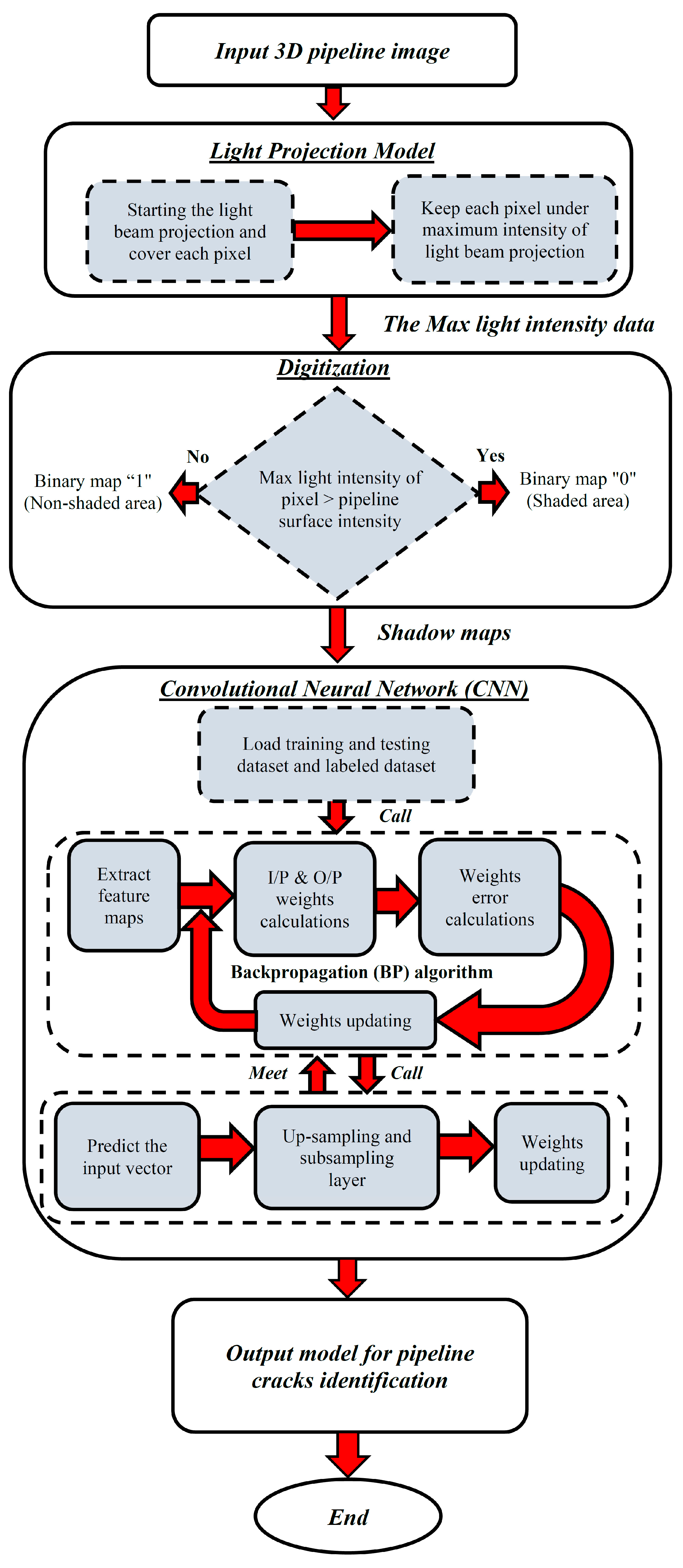
2. Methodology
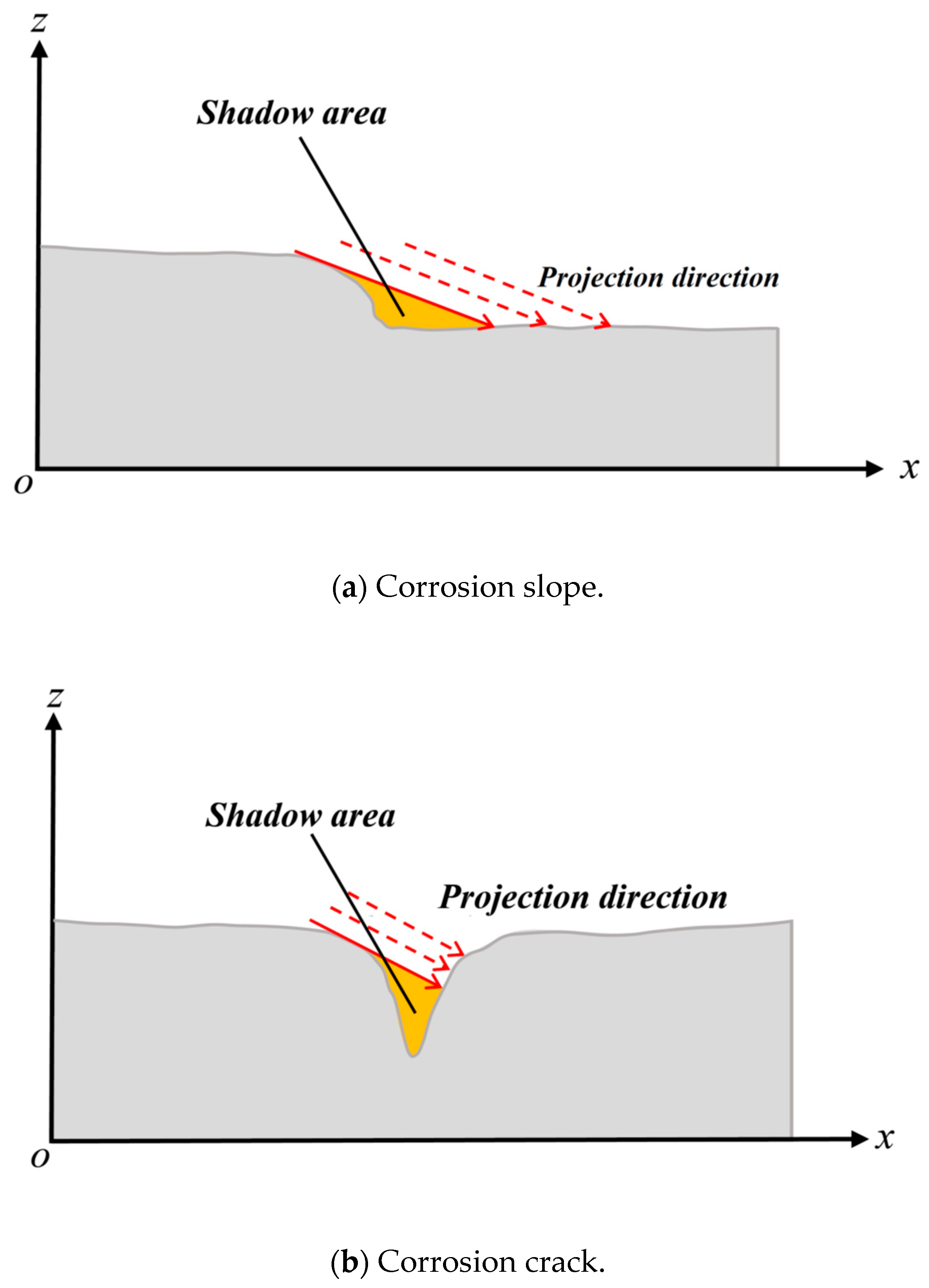
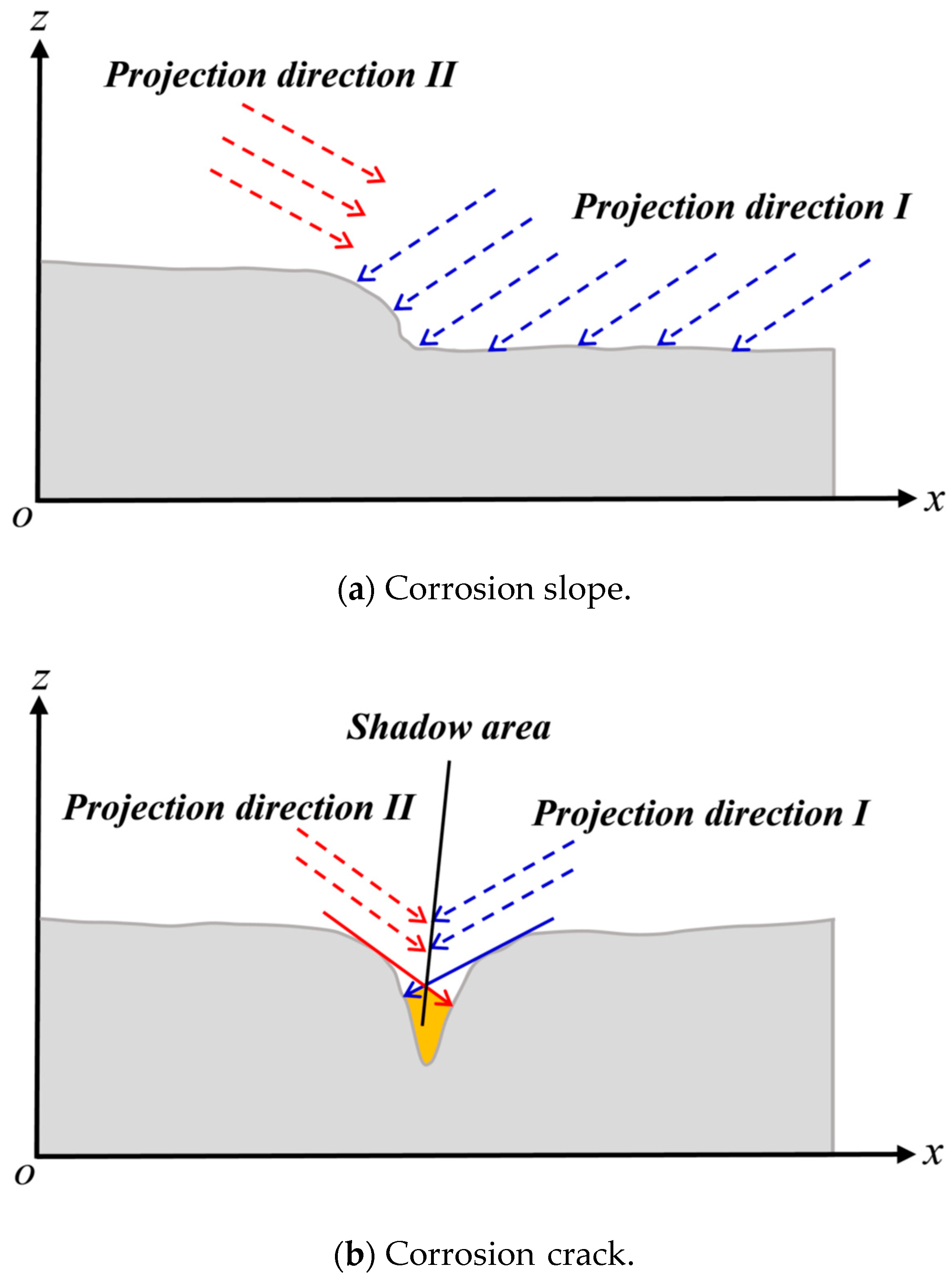
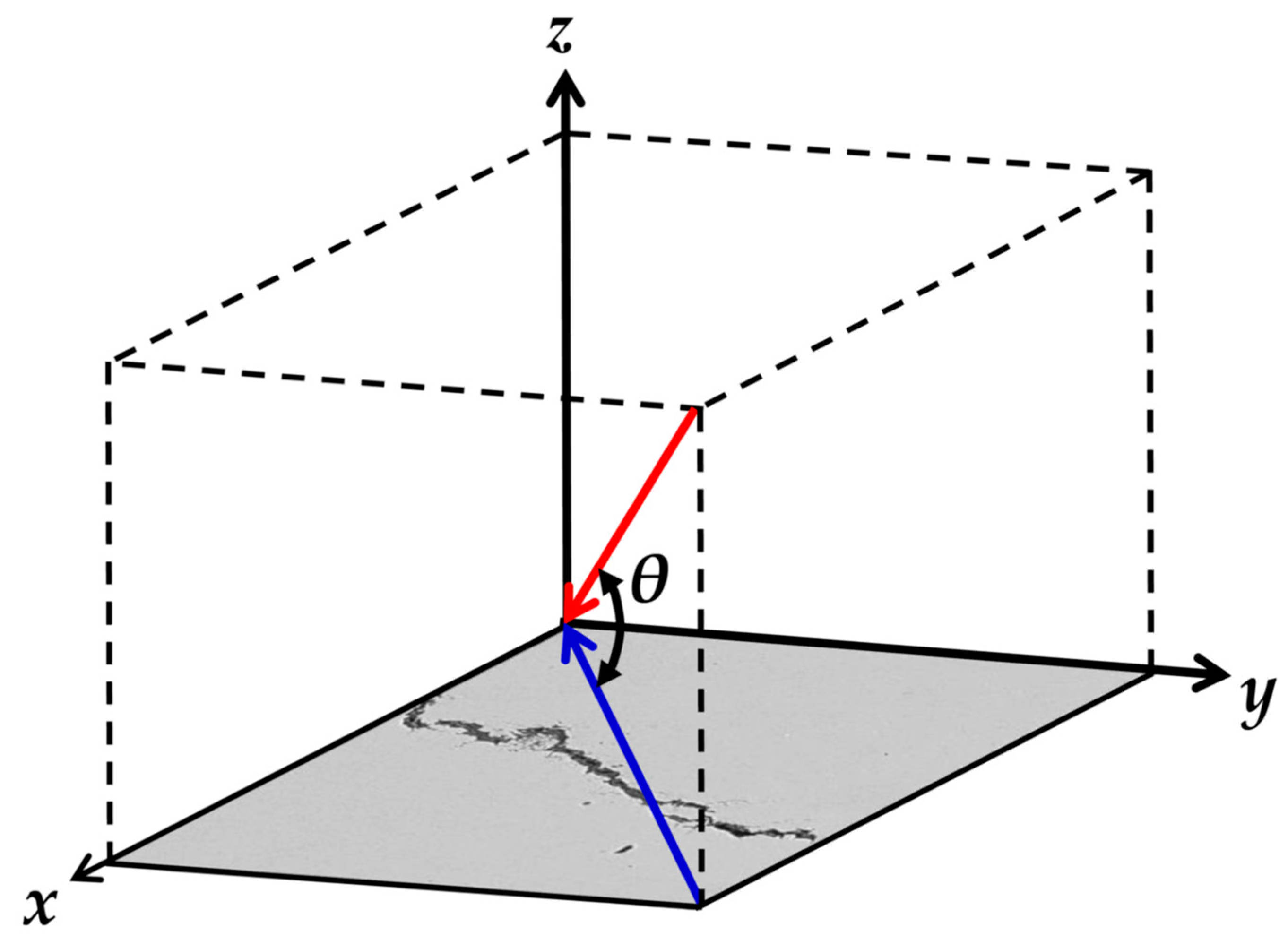
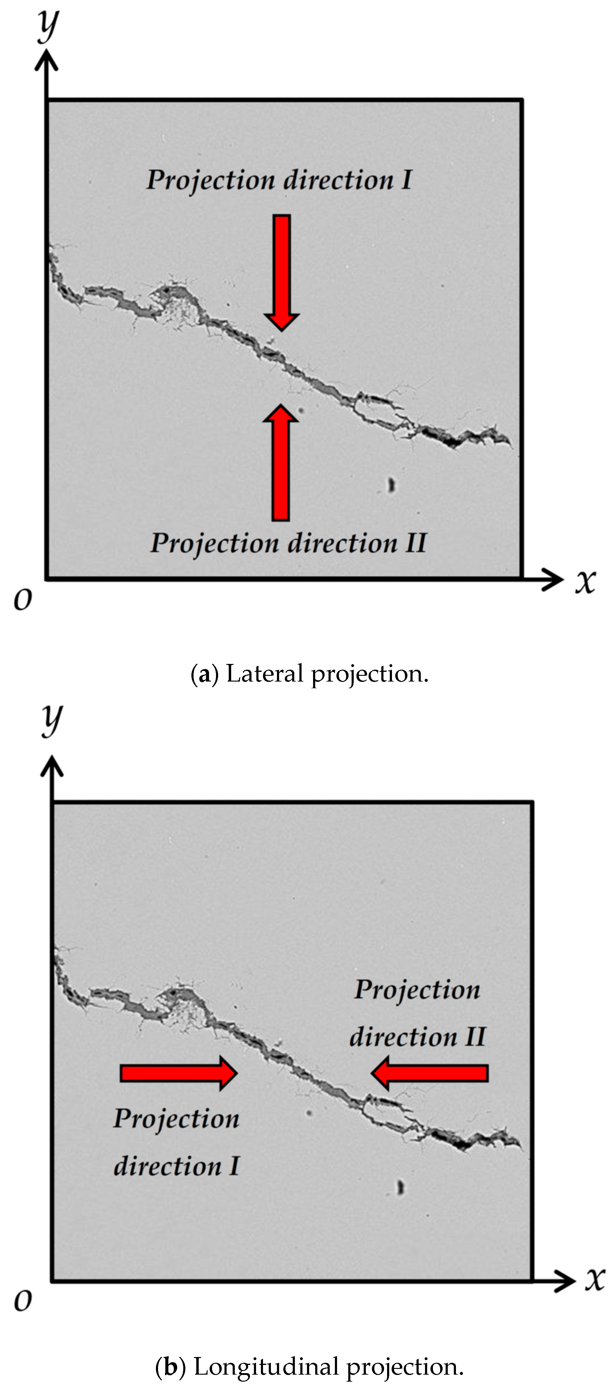
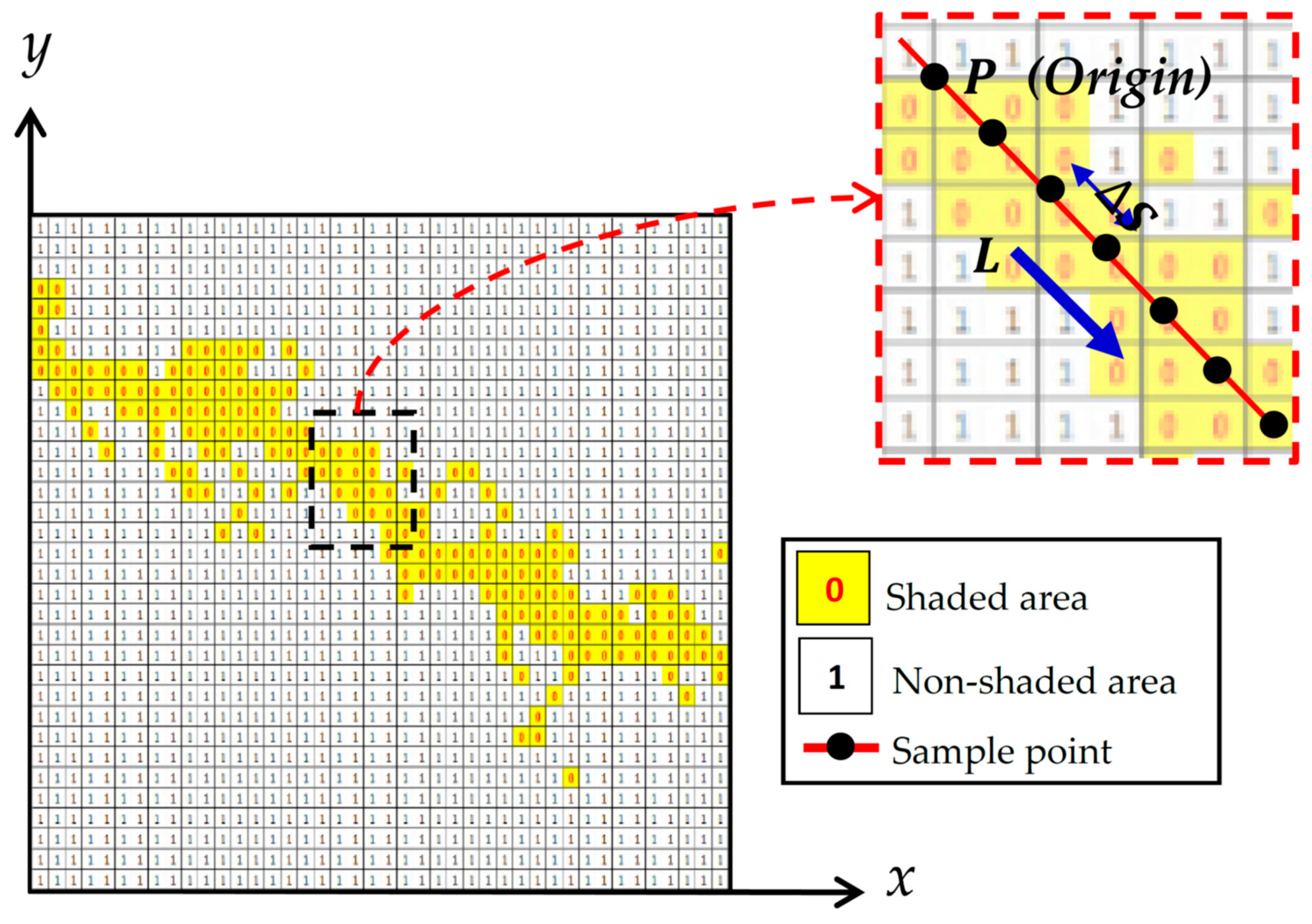
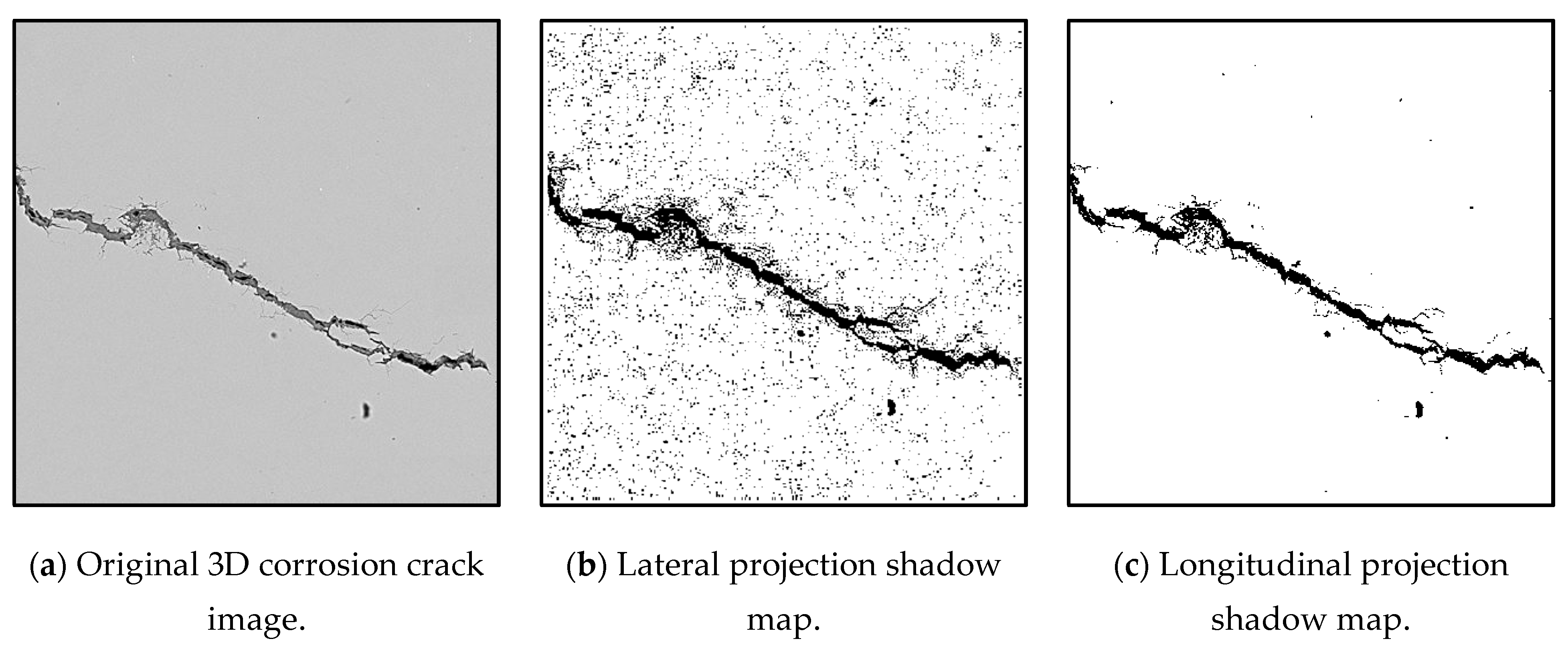
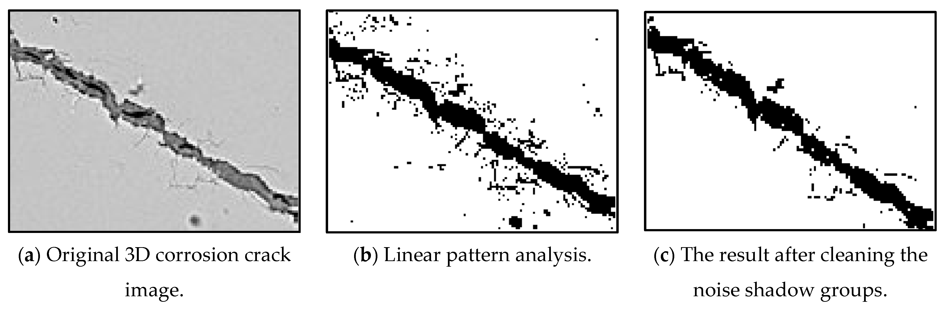
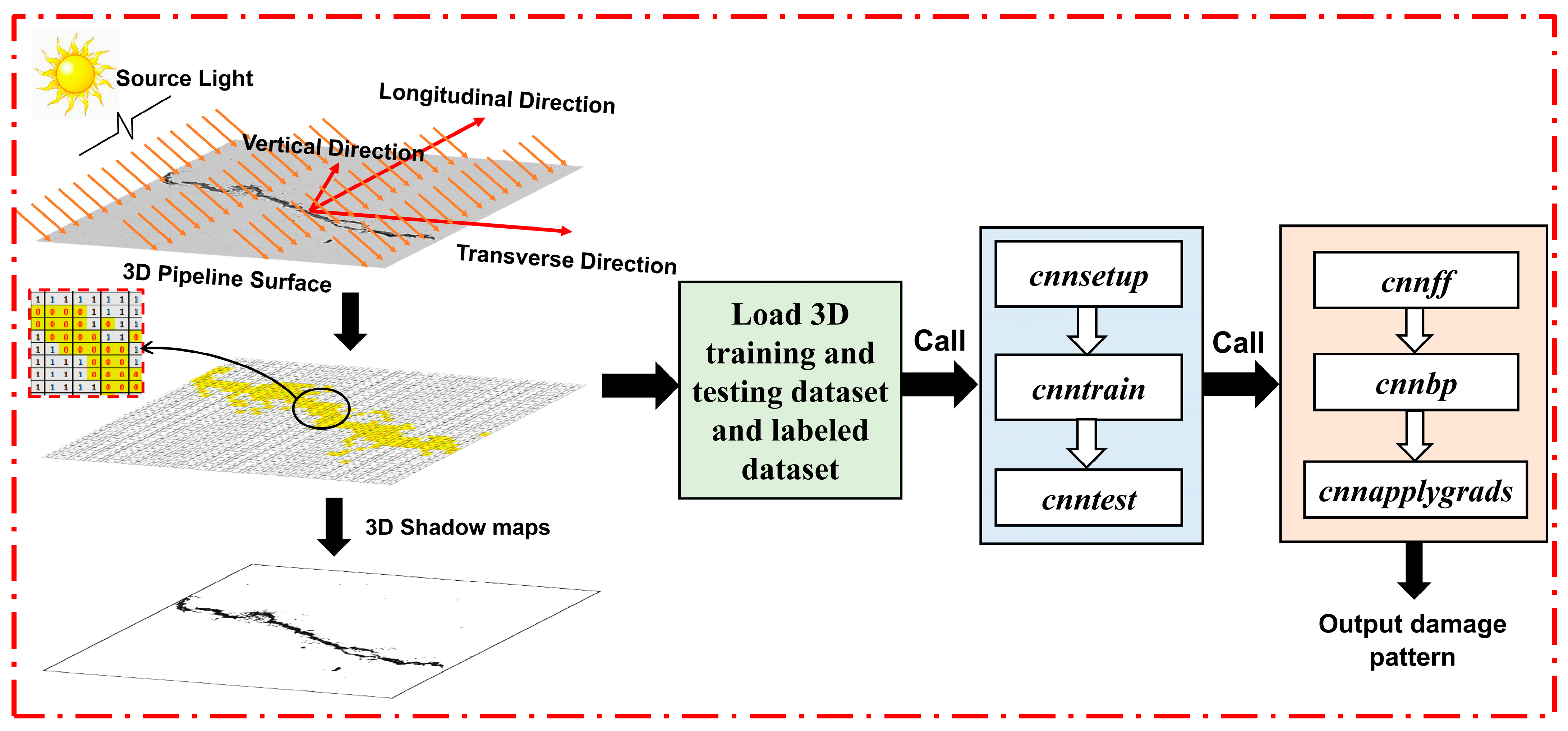
3. Three-Dimensional (3D) Shadow Modeling
- The projected light source (in this work, the high intensity light torches) is infinite and projected light beams are parallel;
- The diffusion, reflection and refraction of light are ignorable.
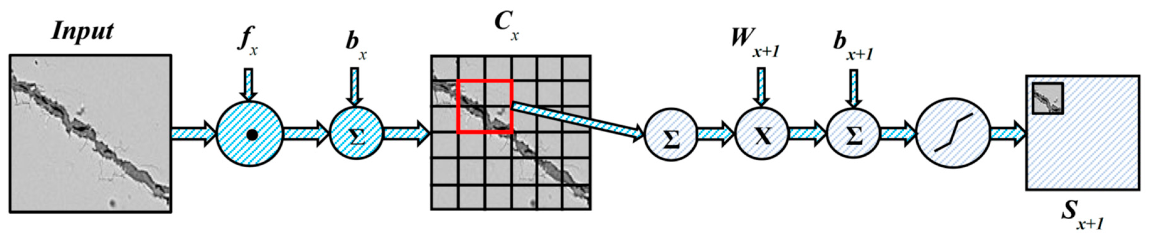
4. Convolutional Neural Network (CNN)
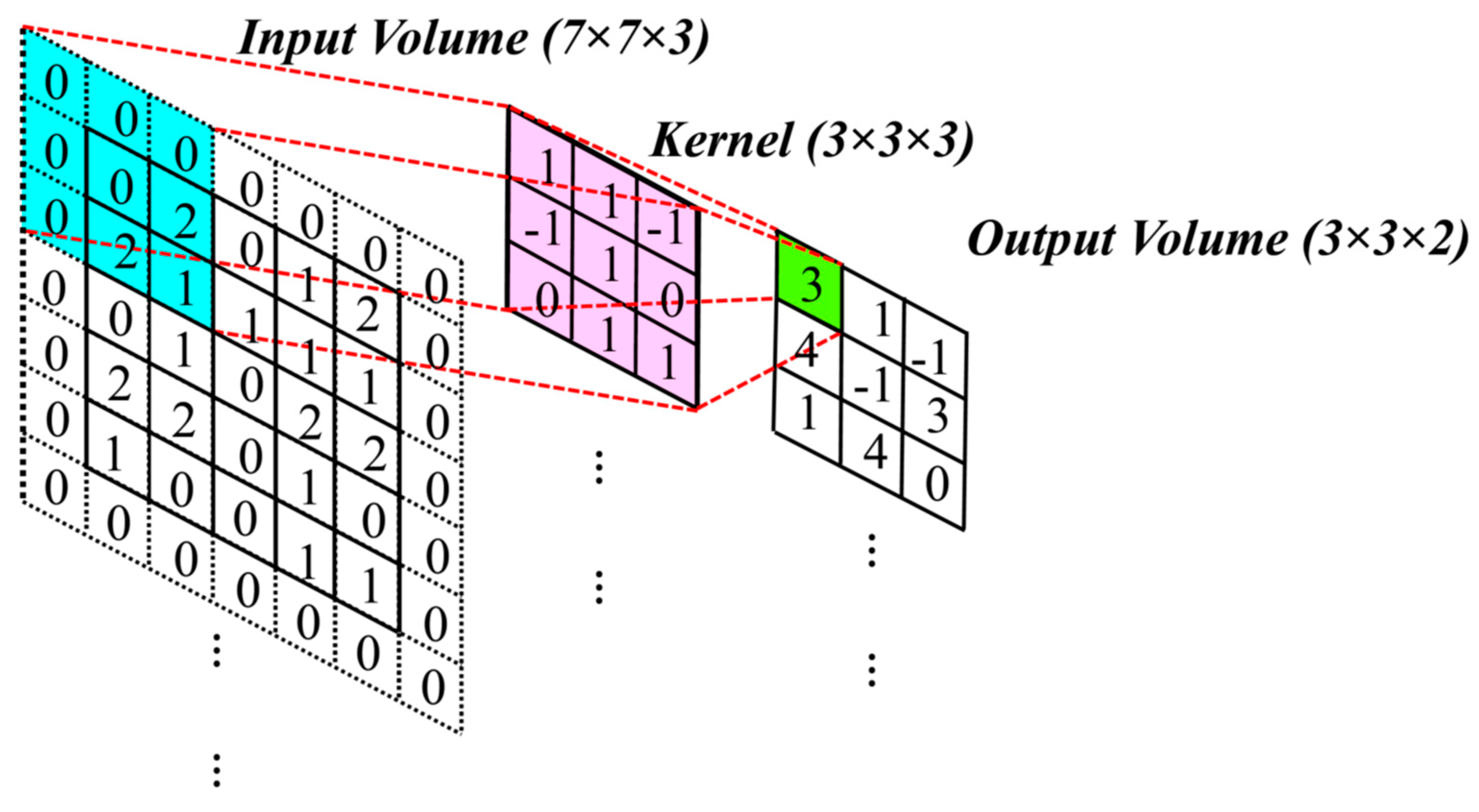
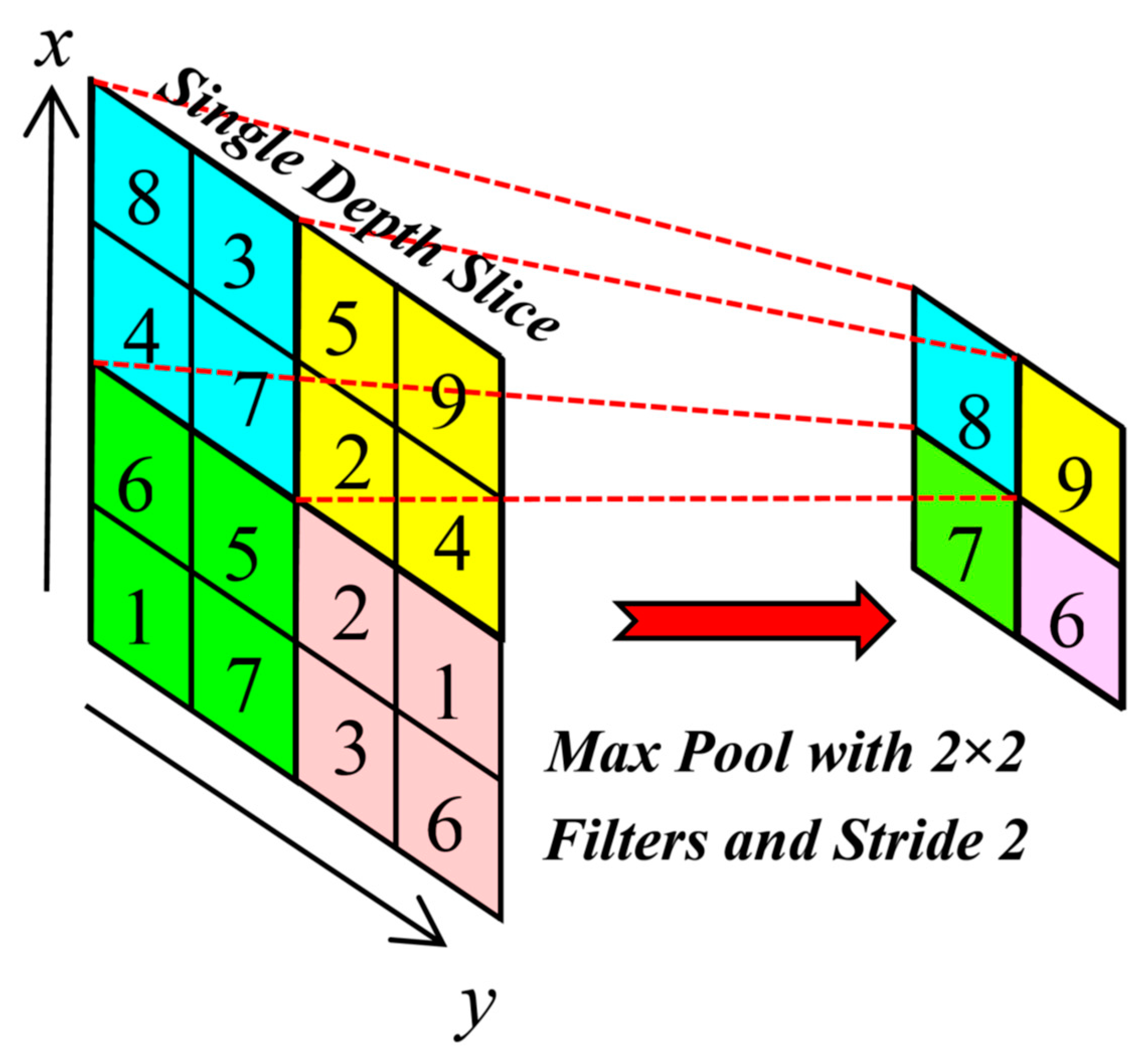
4.1. Convolution Layers and Sub-Sampling Layers
4.2. Learning Combinations of Feature Maps
4.3. Enforcing Sparse Combinations
5. Results and Discussions
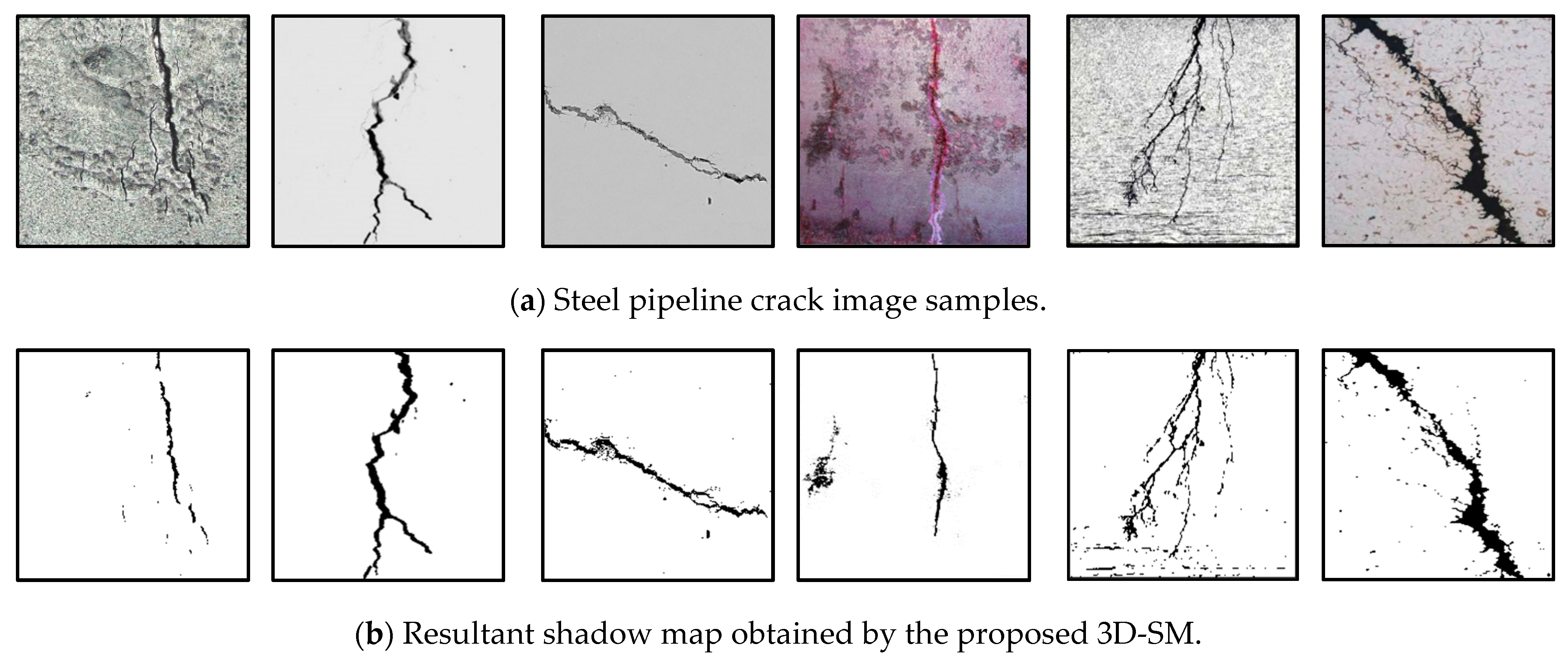
5.1. 3D Crack Images Database
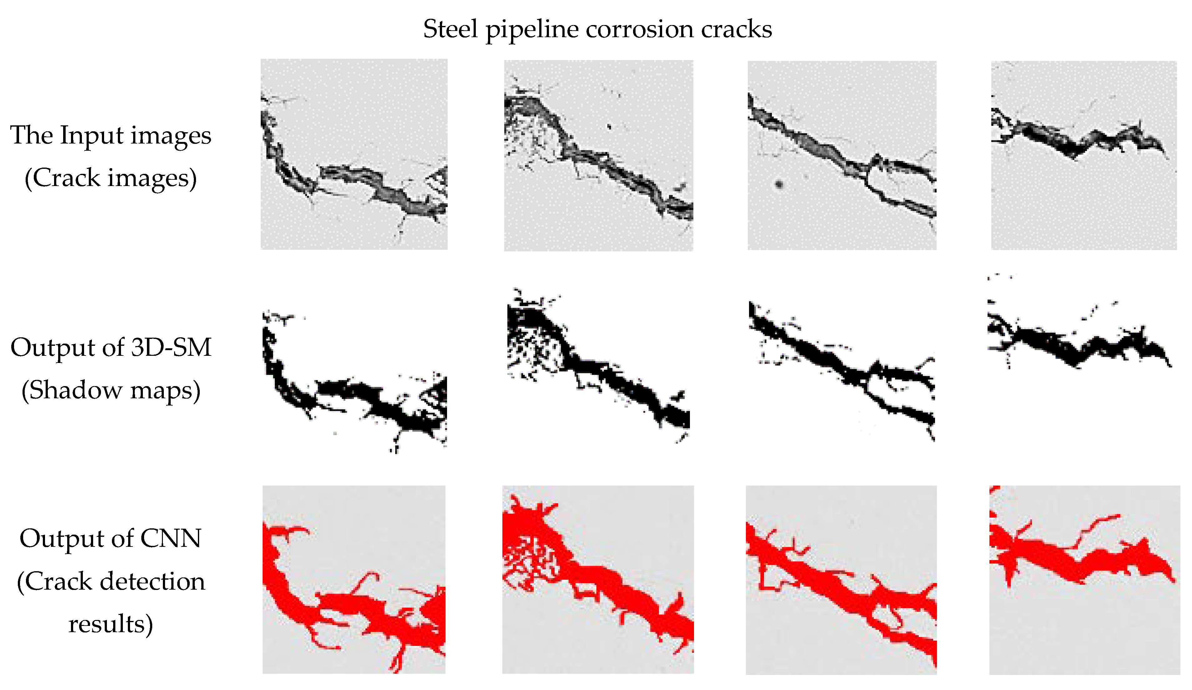
5.2. Pipeline Corrosion Cracks Identification Using CNN
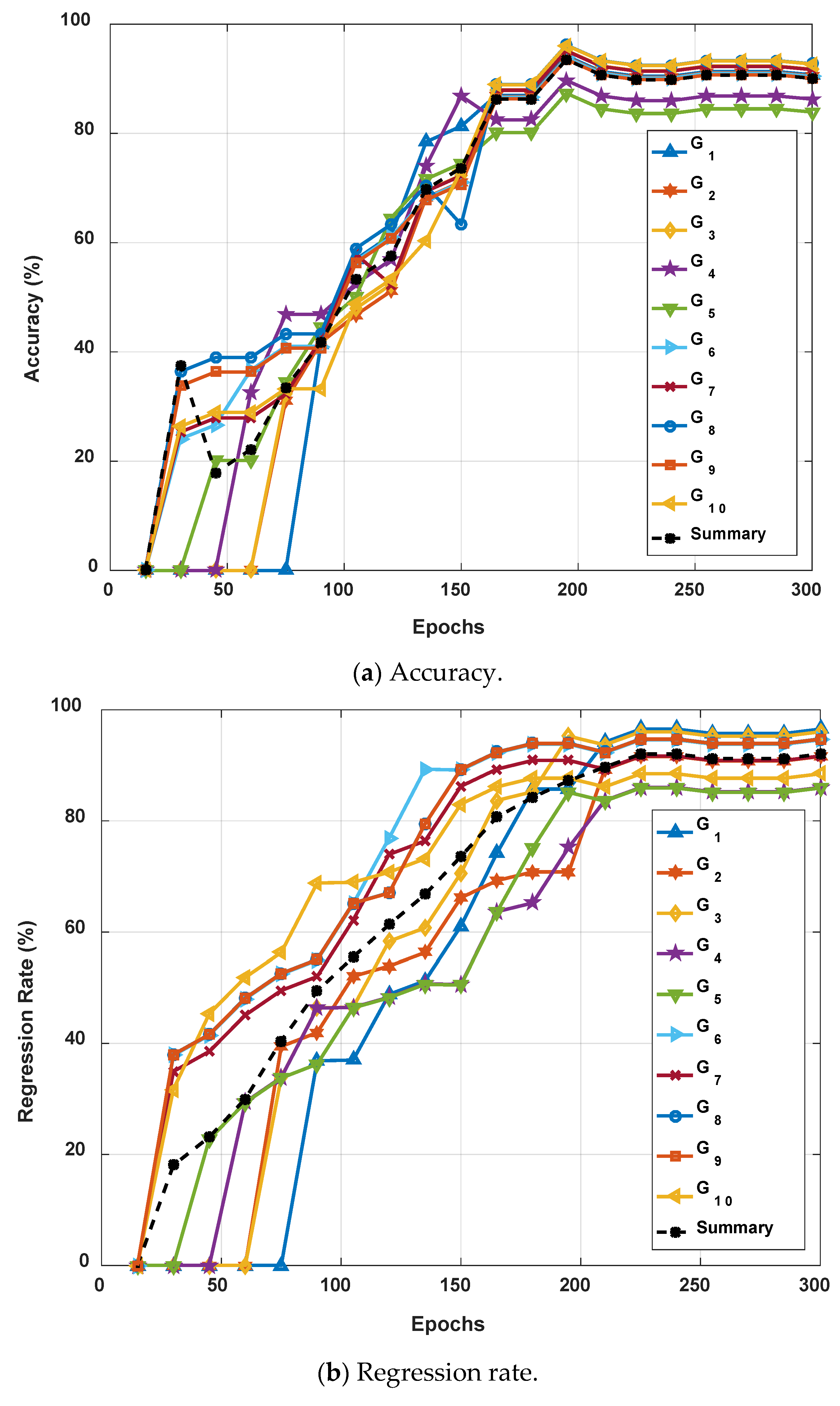
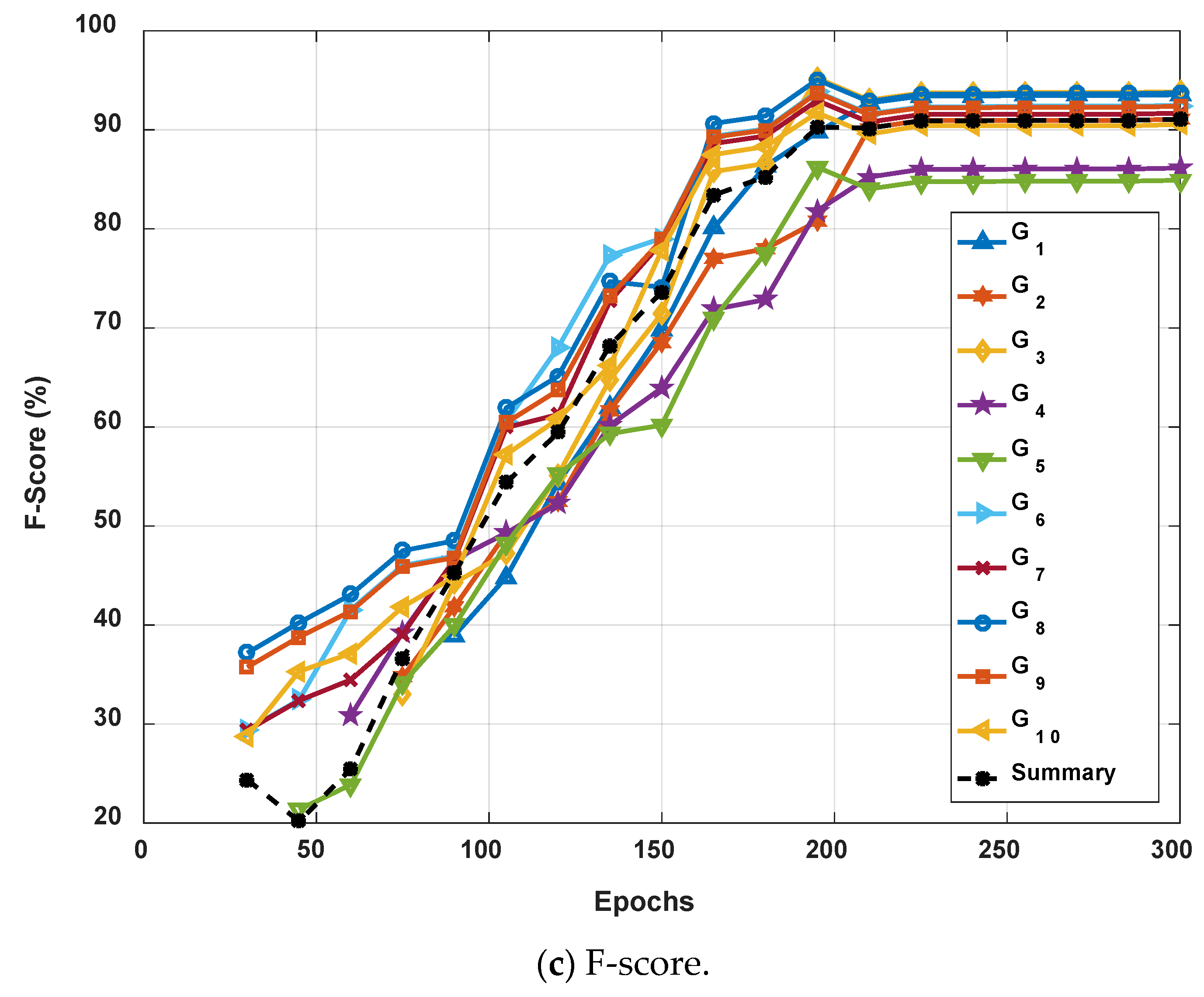
5.3. Evaluation of Accuracy and Reliability of the Present Algorithm
6. Conclusions
Author Contributions
Funding
Institutional Review Board Statement
Informed Consent Statement
Data Availability Statement
Conflicts of Interest
Abbreviations
| The binary value of the integrated shadow map | |
| The binary value of the point in the horizontal shadow map | |
| The binary value of the point in the vertical shadow map | |
| The integrated shadow map | |
| The aspect ratio of the shadow group | |
| The total length of the shadow group | |
| The average width of the shadow group | |
| The aspect ratio threshold, | |
| The average profile width difference rate of shadow group | |
| The total number of profiles of shadow group | |
| The width of the jth section of shadow group | |
| The threshold value of the average profile width difference rate, | |
| The current direction of the third section of shadow group | |
| The next direction of the jth section of shadow group | |
| The center point of the section of shadow group | |
| The center point of shadow group | |
| The average direction difference threshold, | |
| A set of input feature maps. | |
| The bias for each output feature map. | |
| n | The subsampling layer number. |
| An operation of up-sampling which tiles each pixel in the input horizontally and vertically times in the output if the subsampling layer subsamples by a factor of . | |
| The bias. | |
| The kernel weight. | |
| The patch in multiplied by via the element-wise procedure to calculate the element at in the output map in the convolutional layer. | |
| The input maps in the convolutional layer. | |
| A sub-sampling procedure. | |
| and | The bias parameters. |
| The accuracy rate | |
| The regression rate | |
| F- score | |
| 3D-SM | Three-dimensional Shadow Modeling |
| CNN | Convolutional Neural Network |
| SHM | Structural Health Monitoring |
| I/P | Input |
| O/P | Output |
| The number of true-positive elements | |
| The number of false-positive elements | |
| The number of false-negative elements |
References
- Altabey, W.A. FE and ANN model of ECS to simulate the pipelines suffer from internal corrosion. Struct. Monit. Maint. 2016, 3, 297–314. [Google Scholar] [CrossRef]
- He, Y. Corrosion Monitoring, Reference Module in Materials Science and Materials Engineering; Science Direct: Amsterdam, The Netherlands, 2015. [Google Scholar]
- Cole, I.S.; Marney, D. The science of pipe corrosion: A review of the literature on the corrosion of ferrous metals in soils. Corros. Sci. 2012, 56, 5–16. [Google Scholar] [CrossRef]
- Alwis, L.; Sun, T.; Grattan, K.T.V. Optical fibre-based sensor technology for humidity and moisture measurement: Review of recent progress. Measurement 2013, 46, 4052–4074. [Google Scholar] [CrossRef]
- Dong, S.; Liao, Y.; Tian, Q. Intensity-based optical fiber sensor for monitoring corrosion of aluminum alloys. Appl. Opt. 2005, 44, 5773–5777. [Google Scholar] [CrossRef]
- Altabey, W.A.; Noori, M. Detection of Fatigue Crack in Basalt FRP Laminate Composite Pipe using Electrical Potential Change Method. J. Phys. Conf. Ser. 2017, 842, 012079. [Google Scholar] [CrossRef]
- Altabey, W.A. Delamination evaluation on basalt FRP composite pipe by electrical potential change. Adv. Aircr. Spacecr. Sci. 2017, 4, 515–528. [Google Scholar] [CrossRef]
- Altabey, W.A.; Noori, M.; Alarjani, A.; Zhao, Y. Tensile creep monitoring of basalt fiber-reinforced polymer plates via electrical po-tential change and artificial neural network. Sci. Iran. Int. J. Sci. Technol. Trans. Mech. Eng. B 2020, 27, 1995–2008. [Google Scholar] [CrossRef]
- Altabey, W.A. EPC method for delamination assessment of basalt FRP pipe: Electrodes number effect. Struct. Monit. Maint. 2017, 4, 69–84. [Google Scholar] [CrossRef]
- Altabey, W.A.; Mohammad, N. Monitoring the water absorption in GFRE pipes via an electrical capacitance sensors. Adv. Aircr. Spacecr. Sci. 2018, 5, 411–434. [Google Scholar] [CrossRef]
- Altabey, W.A.; Noori, M.; Alarjani, A.; Zhao, Y. Nano-Delamination Monitoring of BFRP Nano-Pipes of Electrical Potential Change with ANNs. Adv. Nano Res. 2020, 9, 1–13. [Google Scholar] [CrossRef]
- Zhao, Y.; Noori, M.; Altabey, W.A.; Wu, Z. Fatigue damage identification for composite pipeline systems using electrical capacitance sensors. Smart Mater. Struct. 2018, 27, 085023. [Google Scholar] [CrossRef]
- Kumar, R.; Ismail, M.; Zhao, W.; Noori, M.; Yadav, A.R.; Chen, S.; Singh, V.; Altabey, W.A.; Silik, A.I.H.; Kumar, G.; et al. Damage detection of wind turbine system based on signal processing approach: A critical review. Clean Technol. Environ. Policy 2021, 23, 561–580. [Google Scholar] [CrossRef]
- Wang, H.; Zhu, N.; Wang, Q. Segmentation of pavement cracks using differential box-counting sppmach. J. Harbin Inst. Technol. 2007, 39, 142–144. [Google Scholar]
- Martin, D.R.; Fowlkes, C.C.; Malik, J. Learning to detect natural image boundaries using local brightness, color, and texture cues. IEEE Trans. Pattern Anal. Mach. Intell. 2004, 26, 530–549. [Google Scholar] [CrossRef]
- Stahl, J.S.; Wang, S. Edge grouping combining boundary and region information. IEEE Trans. Image Process. 2007, 16, 2590–2606. [Google Scholar] [CrossRef] [Green Version]
- Ghiasi, R.; Ghasemi, M.R.; Noori, M.; Altabey, W. A non-parametric approach toward structural health monitoring for processing big data collected from the sensor network. Structural Health Monitoring 2019: Enabling Intelligent Life-Cycle Health Management for Industry Internet of Things (IIOT). In Proceedings of the 12th International Workshop on Structural Health Monitoring (IWSHM 2019), Stanford, CA, USA, 10–12 September 2019. [Google Scholar] [CrossRef]
- Ghiasi, R.; Noori, M.; Altabey, W.A.; Silik, A.; Wang, T.; Wu, Z. Uncertainty Handling in Structural Damage Detection via Non-Probabilistic Meta-Models and Interval Mathematics, a Data-Analytics Approach. Appl. Sci. 2021, 11, 770. [Google Scholar] [CrossRef]
- Zhao, Y.; Noori, M.; Altabey, W.A.; Ghiasi, R.; Wu, Z.; Noori, M. Deep Learning-Based Damage, Load and Support Identification for a Composite Pipeline by Extracting Modal Macro Strains from Dynamic Excitations. Appl. Sci. 2018, 8, 2564. [Google Scholar] [CrossRef] [Green Version]
- Wang, T.; Altabey, W.A.; Noori, M.; Ghiasi, R. A Deep Learning Based Approach for Response Prediction of Beam-Like Structures. Struct. Durab. Health Monit. 2020, 14, 315–388. [Google Scholar] [CrossRef]
- Kost, A.; Altabey, W.A.; Noori, M.; Awad, T. Applying Neural Networks for Tire Pressure Monitoring Systems. Struct. Durab. Health Monit. 2019, 13, 247–266. [Google Scholar] [CrossRef] [Green Version]
- Krizhevsky, A.; Sutskever, I.; Hinton, G.E. Imagenet classification with deep convolutional neural networks. Adv. Neural Inf. Process. Syst. 2012, 25, 1097–1105. [Google Scholar] [CrossRef]
- Bouvrie, J. Notes on Convolutional Neural Networks; Center for Biological Learning, Department of Brain and Cognitive Sciences, Massachusetts Institute of Technology: Cambridge, MA, USA, 2006. [Google Scholar]
- Altabey, W.A. Applying deep learning and wavelet transform for predicting the vibration behavior in variable thickness skew composite plates with intermediate elastic support. J. Vibroeng. 2021. [Google Scholar] [CrossRef]
- Altabey, W.A. Free vibration of basalt fiber reinforced polymer (FRP) laminated variable thickness plates with intermediate elastic support using finite strip transition matrix (FSTM) method. J. Vibroeng. 2017, 19, 2873–2885. [Google Scholar] [CrossRef] [Green Version]
- Altabey, W.A. Prediction of natural frequency of basalt fiber reinforced polymer (FRP) laminated variable thickness plates with intermediate elastic support using artificial neural networks (ANNs) method. J. Vibroeng. 2017, 19, 3668–3678. [Google Scholar] [CrossRef] [Green Version]
- Altabey, W.A. High performance estimations of natural frequency of basalt FRP laminated plates with intermediate elastic support using response surfaces method. J. Vibroeng. 2018, 20, 1099–1107. [Google Scholar] [CrossRef] [Green Version]
- Altabey, W.A. Vibration analysis of laminated composite variable thickness plate using finite strip transition matrix technique. In MATLAB Verifications MATLAB—Particular for Engineer; Bennett, K., Ed.; IntechOpen: Monterey, CA, USA, 2014; Volume 21, pp. 583–620. ISBN 980-953-307-1128-8. [Google Scholar] [CrossRef] [Green Version]
- Abdeljaber, O.; Avci, O.; Kiranyaz, S.; Gabbouj, M.; Inman, D.J. Real-time vibration-based structural damage detection using one-dimensional convolutional neural networks. J. Sound Vib. 2017, 388, 154–170. [Google Scholar] [CrossRef]
- Zhao, Y.; Noori, M.; Altabey, W.A. Damage detection for a beam under transient excitation via three different algorithms. Struct. Eng. Mech. 2017, 63, 803–817. [Google Scholar] [CrossRef]
- Zhao, Y.; Noori, M.; Noori, M.; Awad, T. A Comparison of Three Different Methods for the Identification of Hysterically Degrading Structures Using BWBN Model. Front. Built Environ. 2019, 4, 80. [Google Scholar] [CrossRef] [Green Version]
- Noori, M.; Haifegn, W.; Altabey, W.A.; Silik, A.I.H. A Modified Wavelet Energy Rate Based Damage Identification Method for Steel Bridges. Sci. Iran. Int. J. Sci. Technol. Trans. Mech. Eng. B 2018, 25, 3210–3230. [Google Scholar] [CrossRef] [Green Version]
- Zhao, Y.; Noori, M.; Noori, M.; Beheshti-Aval, S.B. Mode shape-based damage identification for a reinforced concrete beam using wavelet coefficient differences and multiresolution analysis. Struct. Control. Health Monit. 2017, 25, e2041. [Google Scholar] [CrossRef]
- Silik, A.; Noori, M.; Altabey, W.A.; Ghiasi, R. Selecting optimum levels of wavelet multi-resolution analysis for time-varying signals in structural health monitoring. Struct. Control. Health Monit. 2021, in press. [Google Scholar] [CrossRef]
- Silik, A.; Noori, M.; Altabey, W.A.; Ghiasi, R.; Wu, Z. Comparative Analysis of Wavelet Transform for Time-Frequency Analysis and Transient Localization in Structural Health Monitoring. Struct. Durab. Health Monit. 2021, 15, 1–22. [Google Scholar] [CrossRef]
- Silik, A.; Noori, M.; Altabey, W.; Dang, J.; Ghiasi, R.; Wu, Z. Optimum wavelet selection for nonparametric analysis toward structural health monitoring for processing big data from sensor network: A comparative study. Struct. Health Monit. 2021, in press. [Google Scholar] [CrossRef]
- Silik, A.; Noori, M.; Altabey, W.A. Analytic Wavelet Selection for Time—Frequency Analysis of Big Data Form Civil Structure Monitoring. In Civil Structural Health Monitoring, Proceedings of CSHM-8 Workshop 2021; Rainieri, C., Fabbrocino, G., Caterino, N., Eds.; Springer: Berlin/Heidelberg, Germany, 2021; Chapter 29. [Google Scholar] [CrossRef]
- Liang, Y.; Wu, D.; Liu, G.; Li, Y.; Gao, C.; Ma, Z.J.; Wu, W. Big data-enabled multiscale serviceability analysis for aging bridges. Digit. Commun. Netw. 2016, 2, 97–107. [Google Scholar] [CrossRef] [Green Version]
- Wang, T.; Noori, M.; Altabey, W.A. Identification of cracks in an Euler—Bernoulli beam using Bayesian inference and closed-form solution of vibration modes. Proc. Inst. Mech. Eng. Part L J. Mater. Des. Appl. 2021, 235, 421–438. [Google Scholar] [CrossRef]
- Wang, T.; Noori, M.; Altabey, W.A.; Li, Z. Parameter Identification and Dynamic Response Analysis of a Modified Prandtl-Ishlinskii Asymmetric Hysteresis Model via Least-Mean Square algorithm and Particle Swarm Optimization. Proc. IMechE Part L J. Mater. Des. Appl. 2021. [Google Scholar] [CrossRef]
- Li, Z.; Noori, M.; Zhao, Y.; Wan, C.; Feng, D.; Altabey, W.A. A multi-objective optimization algorithm for Bouc–Wen–Baber–Noori model to identify re-inforced concrete columns failing in different modes. Proc. IMechE Part L J. Mater. Des. Appl. 2021. [Google Scholar] [CrossRef]
- Zhao, Y.; Noori, M.; Altabey, W.A.; Reaching Law Based Sliding Mode Control for a Frame Structure under Seismic Load. Earthq. Eng. Eng. Vib. 2021. In press. Available online: https://www.springer.com/journal/11803 (accessed on 18 June 2021).
- Zhao, Y.; Noori, M.; Altabey, W.A.; Lu, N. Reliability Evaluation of a Laminate Composite Plate Under Distributed Pressure Using a Hybrid Response Surface method. Int. J. Reliab. Qual. Saf. Eng. 2017, 24, 1750013. [Google Scholar] [CrossRef]
- Grama, A.; Gupta, A.; Karypis, G.; Kumar, V.; Grama, A. Introduction to Parallel Computing, 2nd ed.; Addison Wesley: Boston, MA, USA, 2003; pp. 209–210. [Google Scholar]
- Davis, J.; Goadrjch, M. The relationship between precision-recall and ROC curves. In Proceeding of the 23rd International Conference on Machine Learning, Pittsburgh, PA, USA, 25–29 June 2006; ACM: New York, NY, USA, 2006; pp. 233–240. [Google Scholar]
- Fawcetr, T. An introduction to ROC analysis. Pattern Recognit. Lett. 2006, 27, 861–874. [Google Scholar] [CrossRef]

| Cnnsetup | The Cnnsetup is used to set up the feature maps, The kernel window is composed of elements with the size of kernelsize × kernelsize. Each element is an independent weight. |
| cnntrain | The cnntrain is used to reorder the sample, and randomly train and calculate the weights of network input and output. Then, the derivative of the error is calculated with respect to weights by the back propagation (BP) algorithm. |
| Cnnff | The Cnnff uses the neural network to predict the input vector. The samples are first reordered and then randomly trained. |
| cnnbp | The cnnbp layer is used for up-sampling and subsampling layer is used for down-sampling. |
| Cnnapplygrads | The Cnnapplygrads is used for updating of the weight depending on training, testing, labeled training, and labeled testing datasets. |
| Layer | Kernel Size | Number of Parameter | Number of Connection |
|---|---|---|---|
| C1 | 12 × 12 | 580 | 16,369,920 |
| S2 | 6 × 12 | 4 | 383,616 |
| C3 | 12 × 12 | / | / |
| S4 | 6 × 6 | / | / |
| Group No. | Image Number Range | Accuracy (%) | Regression Rate (%) | F-Score (%) |
|---|---|---|---|---|
| 1 | 94.17 | 96.53 | 85.4 | |
| 2 | 93.97 | 91.61 | 85.27 | |
| 3 | 95.19 | 96.05 | 90.28 | |
| 4 | 89.71 | 86.02 | 90.18 | |
| 5 | 87.35 | 85.93 | 91.92 | |
| 6 | 93.86 | 94.61 | 94.47 | |
| 7 | 95.12 | 91.69 | 92.96 | |
| 8 | 96.18 | 94.76 | 93.85 | |
| 9 | 93.56 | 94.73 | 94.39 | |
| 10 | 96.14 | 88.49 | 93.06 | |
| Summary | 93.53 | 92.04 | 91.18 |
Publisher’s Note: MDPI stays neutral with regard to jurisdictional claims in published maps and institutional affiliations. |
© 2021 by the authors. Licensee MDPI, Basel, Switzerland. This article is an open access article distributed under the terms and conditions of the Creative Commons Attribution (CC BY) license (https://creativecommons.org/licenses/by/4.0/).
Share and Cite
Altabey, W.A.; Noori, M.; Wang, T.; Ghiasi, R.; Kuok, S.-C.; Wu, Z. Deep Learning-Based Crack Identification for Steel Pipelines by Extracting Features from 3D Shadow Modeling. Appl. Sci. 2021, 11, 6063. https://doi.org/10.3390/app11136063
Altabey WA, Noori M, Wang T, Ghiasi R, Kuok S-C, Wu Z. Deep Learning-Based Crack Identification for Steel Pipelines by Extracting Features from 3D Shadow Modeling. Applied Sciences. 2021; 11(13):6063. https://doi.org/10.3390/app11136063
Chicago/Turabian StyleAltabey, Wael A., Mohammad Noori, Tianyu Wang, Ramin Ghiasi, Sin-Chi Kuok, and Zhishen Wu. 2021. "Deep Learning-Based Crack Identification for Steel Pipelines by Extracting Features from 3D Shadow Modeling" Applied Sciences 11, no. 13: 6063. https://doi.org/10.3390/app11136063
APA StyleAltabey, W. A., Noori, M., Wang, T., Ghiasi, R., Kuok, S.-C., & Wu, Z. (2021). Deep Learning-Based Crack Identification for Steel Pipelines by Extracting Features from 3D Shadow Modeling. Applied Sciences, 11(13), 6063. https://doi.org/10.3390/app11136063