Finding Location Visiting Preference from Personal Features with Ensemble Machine Learning Techniques and Hyperparameter Optimization

Abstract

For the question regarding the relationship between personal factors and location selection, many researches support the effect of personal features for personal location favorite. However, it is also found that not all of personal factors are effective for location selection. In this research, only distinguished personal features excluding meaningless features are used in order to predict visiting ratio of specific location categories by using three different machine learning techniques: Random Forest, XGBoost, and Stacking. Through our research, the accuracy of prediction of visiting ratio to a specific location regarding personal features are analyzed. Personal features and visited location data had been collected by tens of volunteers for this research. Different machine learning methods showed very similar tendency in prediction accuracy. As well, precision of prediction is improved by application of hyperparameter optimization which is a part of AutoML. Applications such as location based service can utilize our result in a way of location recommendation and so on.

1. Introduction

Prior researches show that human personality and favorite visiting place have considerable relationship . Coefficient of Determination is used in the relation between personality and favored locations [1]. By use of probability models such as Poisson distribution, the relation between personality and favored locations are identified and personal mobility model is predicted in [2,3]. These are traditional methods of analysis based on statistics. A trail to use machine learning in order to these analysis can be found in [4] in terms of back propagation network. Nowadays, a lot of new methods including machine learning technologies can be adopted for such sort of analysis. In this research, we will show the relation between personal factors and favorite locations using various machine learning techniques, especially ensemble techniques, and will verify the consensus of results from machine learning methods.

Ensemble techniques combines the result of each independent model and thus shows more preciseness comparing to single model only. By introducing up to date machine learning techniques, ensemble techniques of several machine learning models are used in this research. Two representative ensemble techniques are used: bagging and boosting. For bagging techniques, random forest is used since it is widely used. For boosting techniques, we used XGBoost since it has high performance and fast in training time, which is also widely used. Both of two methods, random forest and XGBoost have base model of decision tree. We also used stacking as shown in Section 2.4 in order to verify that various regression models other than decision tree also effective in our research in a form of meta learning. Different from previous researches, our focus is that common belief of relationship between personality and location selection is proved by state of the art technologies. As well personal features other than personality such as age, religion, method of transportation, salary, and so on, are also used for this relationship analysis. In addition, the results of ensemble methods will be presented in numerical manner. For the inputs of analysis, as well as personalities, other personal factors such as salary, method of transportation, religion, and so on are found to be related with favorite locations [5,6]. However not all of these personal factors are meaningful factors for location preference. In other words, meaningless features for the input of analysis degrades the prediction accuracy of the relationship. Therefore feature selection [7] was executed for each location category. And then, prediction accuracy was improved through hyperparameter optimization. Hyperparameter optimization was done in three different ways: grid search, random search [8] and bayesian optimization [9] from the current advancement of AutoML. Grid search and random search are two representative methods of hyperparameter optimization. Grid search takes long time since it checks performance for every possible candidates of parameters. Random search is faster than grid search since it checks several samples randomly while shows less precision comparing to grid search. These two methods has shortages that current search information cannot be transferred to next step. Bayesian optimization overcomes this shortage: it utilizes prior knowledge for new search of optimized value with smaller search time and higher precision. In this research, all three of hyperparameter optimization methods are used. In this research, Big Five Factors (BFF) of personality such as Openness, Conscientiousness, Extraversion, Agreeableness and Neuroticism are used as well as the highest level of education, religion, salary, method of transportation, commute time, the frequency of journey in one year, social media usage status, time spent on social media per day, and nature of personaly hobby. BFF is taxonomy for personality characteristics presented by Costa & McCrae in 1992, and it is found useful for personality related research. In this research, numerical features of BFF is utilized and BFF is regarded as parts of input data. With these selected inputs of relationship analysis, we will use machine learning techniques for the analysis. Basically, three machine learning methods were used: Random Forest, XGBoost, and Stacking. Each of three methods is sort of ensemble techniques. From various aspects of researches, ensemble method is proven to compensate the weakness of single model and improve the performance of generalization [10]. Random Forest, especially, prevents overfitting by using bagging techniques. For XGBoost, boosting technique is used to repeated random sampling for weighted sequential learning. It is also possible to reduce bias with boosting technique. Stacking combines multiple machine learning methods in order to exploit of strength of multiple models and complement weakness of two different models in a way of multistage learning. Stacking has better performance comparing to other models while it requires high computational cost. With these three different ensemble methods with different characteristics, the results of three techniques must be verified each other in order to show the consensus of three result sets. In Section 2, we will show related techniques. In addition to machine learning technique used in this research, considerations of personality factors will be discussed. Section 3 will show details of the data and the experiment. The handling of personal factors and location categories will be discussed. As well, SMAPE will be addressed which stands for prediction error along with search space for hyperparameter optimization. Section 4 will show results of analysis by Random Forest, XGBoost, and Stacking and evaluate the results. Results of all three techniques were verified and discussed. As well, results of feature selection and hyperparameter optimization will be discussed. For Random forest and XGBoost, we can apply both of feature selection and hyperparameter optimization however for Stacking, hyperparamter optimization was omitted due to the high computational cost. However, feature selection solely improved prediction accuracy for most of location category. There is high similarity among three result sets and thus consensus can be addressed for the relationship between location categories and personal features. Section 5 will conclude this research with future works.

2. Related Works

2.1. Ensemble Techniques

Ensemble model is a technique to generate one strong prediction model with combinations of existing several machine learning models, which usually shows better prediction performance comparing to single model approach. Three distinguished models of ensemble methods are bagging, boosting and Stacking. Bagging reduces variance, boosting reduces bias, and stacking shows improved prediction performance. For example, ensemble methods are highly ranked at the machine learning competition such as Netflix competition, KDD 2009, and Kaggle [11]. Random Forest is a typical model using bagging. Boosting algorithm has improved to XGBoost which is usual selection with guaranteed performance nowadays. Stacking combines different models while bagging or boosting depends on single base model. In such way, strength of different algorithms are exploited while weakness of each algorithms can be compensated. We will use all three methods: Random Forest, XGBoost, and Stacking in order to show the relationship between personal features and favorite location categories [10].

2.2. Random Forest

Random Forest is suggested by Leo Breiman in 2001 [12]. Random Forest a combination of different decision trees. Each decision tree can predict well while there is possibility of overfitting for train data. But combination of various independent decision trees and average of the results can show prediction performance excluding overfitting effect. Bootstrap is usually used in order to generate multiple independent trees. Each nodes utilizes part of input features. Each branch of decision tree uses subset of different features. Such a process of learning enables every decision tree in Random Forest be unrelated. Then the final result of regression analysis is average of the results from each decision tree. In this research, we use average while in case of classification problem, the final value can be voted from the results of each decision tree. It is resistant to noise. In addition, the degree of effect of input feature can be numerically represented as importance value. With feature importance, important and effective input features can be selected. It also works well on very large datasets and can parallelize the train simply. It is also appropriate to deal with many input features [13]. Random Forest is one of widely used machine learning algorithm with excellent performance. It works well even without much hyperparameter tuning, and does not need to scale data. However, some of hyperparameters are optimized in order to figure out the effect of hyperparameter. Due to this advantage and performance, a Random Forest was used for this study.

2.3. XGBoost

XGBoost use boosting instead of bagging in terms of ensemble. Boosting is a technique of binding weak leaner in order to build powerful predictor. Other than bagging, which aggregates result of independent models, boosting generates booster which stands for base model sequentially. Bagging is to generate model with general performance while boosting is concentrated on solving difficult problems. Therefore, boosting put high weight on difficult problems, by assigning high weight on incorrect answers while assigning low weight on correct answers. Boosting is prone to be weak with outlier values even though it shows high prediction accuracy.

XGBoost stands for Extreme Gradient Boosting and is developed by Tianqi Chen [14]. XGBoost is a performance upgraded version of Gradient Boosting Machine (GBM). XGBoost is widely used by various challenges such as the Netflix prize. For example, 17 prize winners out of 29 solutions of Kaggle in 2015 is implemented by XGBoost [11]. XGBoost is supervised learning algorithm and is an ensemble method such as Random Forest. It is suitable to regression, classification and so on. XGBoost is aim for scalability, portability, and accurate library. In other words, XGBoost utilizes parallel processing and has high flexibility. It has automatic pruning facility with greedy-algorithm and thus shows less chance of overfitting. XGBoost has various hyperparameters and learning rate, max depth of booster, selection of boosters, number of booster are very effective parameters for performance. For boosters of XGBoost, there are gbtree, gblinear, and dart. Gbtree utilizes weak learner as regression tree which is a decision tree with continuous real number object values. Gblinear utilizes weak learner as linear regression model, and dart has base model of regression tree with dropout which is usually used in neural network.

2.4. Stacked Generalization (Stacking)

Stacking is one of ensemble method of machine learning method supposed by D. H. Wolperk dates in the year of 1992 [15]. The key of Stacking is training various machine learning models independently, and then meta model does machine learning with the result of the models as inputs, thus Stacking has stack of two or more learning phases. Stacking method combines various machine learning models so that it solves high variance problem fulfilling to the basic purpose of ensemble method, different from other machine learning methods such as bagging, boosting, and voting. In addition, combinations were made in a way that to obtain the strength of each models and compensates the weakness of each models.

Training stage is composed of two phases. At level 1, prediction of sub models are trained with train data similar to other methods. Usually various sub models are utilized in order to generate various prediction. At level 2, prediction generated at level 1 are regarded as input features, and then meta learner or blender, which is final predictor, generates final prediction result. In this stage, overfitting and bias are reduced since level 2 uses different train data from level 1 [16]. Since Stacking does not provide feature selection, input features selected by Random Forest model were used. In our research, ExtraTreesRegressor, RandomForestRegressor, XGBRegressor, LinearRegressor, and KNeighborsRegressor are used at level 1, and final results were selected with low error rate from the result of XGBoost and Random Forest depending on each location categories.

2.5. Feature Selection

Usually, machine learning is a linear or non-linear function of input data. The selection of train data in order to learn a function is not negligible for better model construction. The volume of data does not guarantee better models however, incorrect results could be misled. For example, linear function with large number of independent variable does not guarantee high prediction of expected value of dependent variable. In other words, the performance of machine learning is highly dependent on input data set, as meaningless input data hinders learning result from being better one. Therefore, it is required to select meaningful features of collected data in advance to model learning, and it is so called feature selection. Subsets of data is used to test the validity of features, i.e., feature selection. For example, importance of feature is higher as the feature sits near root of tree. Then it is possible to imply the importance of a specific feature. In case of regression model, it is possible to do feature selection with use of forward selection and/or backward elimination. In addition to improve performance of model, feature selection has another benefit of reducing the dimension of input data. Through the feature selection, input data set which is smaller than real observation space however which has better explainability, and it is useful for very big data, or for restricted resource or time [7].

2.6. Hyperparameter Optimization

Apart from parameters dependent on data or model, hyperparameter is dependent on machine learning model. Learning rate for deep learning or max depth for decision tree are prominent examples. It is very important to find optimal value for each hyperparameter since hyperparameters significantly affects the performance of model. Manual search of hyperparameters usually requires intuition of skillful researchers, luck and consumes too much time. There exists two famous systematic methodology called grid search and random search [8]. Grid Search searches hyperparameter values in predefined regular intervals and decide values of highest performance, even though human actions are also required. Such uniform and global nature of grid search is a better than manual search however, also requires much time in case of combination for hyperparameters increase. Random search, a random sampling approach of grid search shows increased speed of hyperparameter search. However, these two search methods does repetitive unnecessary search since they does not utilize prior knowledge of hyperparameter search. Bayesian Optimization is another useful method with systematic use of prior knowledge [9]. Bayesian Optimization assumes an objective function f of input value x, where objective function f is a blackbox and requires time to compute. Searching $x^{*}$ for f with small number of input values as small as possible is main purpose. Surrogate Model and Acquisition Function are also required. Surrogate Model does probabilistic estimation for unknown objective function based on known input values and function values pair of $(x_1,f\left(x_1\right)),\dots ,(x_t,f\left(x_t\right))$. Probability models for surrogate model are Gaussian Processes (GP), Tree-structured Parzen Estimators (TPE), Deep Neural Networks and so on. Acquisition Function recommends next useful input value of $x_{t+1}$ based on current estimations of objective function in order to search optimal input value of $x^{*}$. Two strategies are famous: exploration and exploitation. Exploration recommends points with high standard deviation since $x^{+}$ may exist in uncertain region. Exploitation recommends points around the point with highest function value. Two strategies are equally important in order to search optimal input value, $x^{+}$. However, calibrating ratio of two strategy is very important since these two strategies show trade off. Expected Improvement (EI) is the most frequently used as acquisition function since EI contains both of exploration and exploitation. Probability of improvement (PI) is a probability of a certain input value x which function value is bigger than $f\left(x^{+}\right)={max}_{i}f\left(x_i\right)$ among current estimations of $f\left(x_1\right),\dots ,f\left(x_t\right)$. Then EI calculates the effect of x considering PI and magnitude between $f\left(x\right)$ and $f\left(x^{+}\right)$. EI can consider Probability of Improvement (PI), and another strategies such as Upper Confidence Bound (UCB), Entropy Search (ES), and so on are exist.

2.7. Big Five Factors (BFF)

BFF is a factor of personality suggested by P.T. Costa and R.R. McCrae in 1992 [17]. It has five factors of Openness, Conscientiousness, Extraversion, Agreeableness, and Neuroticism. Set of questionnaires is answered by participants and each five factors will be valued as a score from 1 to 5points. Since BFF can numerically represent conceptual human personality, many of research adopts BFF [18,19,20,21,22,23].

3. Preparation of Experiments

Previous research results showed that various personal factors effect the favorite visiting place [5,6]. In addition, effective personal factors vary widely according to each location category [5]. In this research, more precise experiments were designed including feature selection and hyperparameter optimization with three different machine learning methodology. More than 60 volunteers had been collected their own data for this research. However, some parts of data from volunteers are too small for this research, therefore only meaningful data sets are survived. From the data of 34 volunteers, personal factors used in the experiments were:

• The highest level of education
• Religion
• Salary
• Method of transportation
• Commute time
• The frequency of journey in one year
• Social media usage status
• Time spent on social media per day
• Category of personaly hobby
• BFF

These input features and location visiting data from SWARM [24] application are treated as inputs for Random Forest, XGBoost, and Stacking. The primary result is ratio of visiting to specific location categories. For Stacking, ExtraTreesRegressor, RandomForestRegressor, XGBRegressor, LinearRegressor, and KNeighborsRegressor are used in level 1, and XGBoost and Random Forest are used in level 2, result with the smallest error rate is selected. In order to compare experiment result, Symmetric Mean Absolute Percentage Error (SMAPE) discussed in Section 3.4. SMAPE usually represented in a range of 0 to 200% while we normalized the value in a range of 0 to 100% by revising the formula for intuitive comparison. As a result, prediction accuracy is difference between 100% and value of SMAPE.

3.1. Personal Factors

BFF stands for Big Five Factors where the five factors are Openness (O), Conscientiousness (C), Extraversion (E), Agreeableness (A), and Neuroticism (N). Each factors is measured as numerical numbers so that factors can be easily applied to training process. Table 1 shows BFF of participants. We can figure out personality of a person through these values. Person with high Openness is creative, emotional and interested in arts. Person with high Conscientiousness is responsible, achieving, and restraint. Person with high Agreeableness is agreeable to other person, altruistic, thoughtfulness and modesty. While person with high Neuroticism is sensitive to stress, impulsive, hostile and depressed. For example, as shown in Table 1, person 4 is creative, emotional, responsible, restraint. Also considering person 4’s Neuroticism, person 4 is not impulsive and resistant to stress. The personality shown in Table 1 will be used our experimental basis with other personal factors.

Table 1. BFF of Participants.

	O	C	E	A	N
Person 1	3.3	3.9	3.3	3.7	2.6
Person 2	2.7	3.2	3.2	2.7	2.8
Person 3	4.3	3.1	2.3	3.2	2.9
Person 4	4.2	4.3	3.5	3.6	2.6
Person 5	4	3.7	4	3.9	2.8
Person 6	3.8	4	3.1	3.8	2.3
Person 7	3.2	3.2	3.5	3.3	3.5
Person 8	2.8	3.8	3.8	3.3	2.3
Person 9	3.4	3.6	3.5	3.6	3.1
Person 10	3	3.6	2.5	3	3
Person 11	4.1	3.8	3.8	2.8	3
Person 12	3.1	3	2.8	3	2.8
Person 13	3.3	3.2	3.5	2.6	2.6
Person 14	3.7	3.3	3.6	3.8	3.5
Person 15	2.4	3.7	3	2.8	2.6
Person 16	3.4	3.2	3.0	3	2.6
Person 17	3.9	3.3	3.5	2.9	2.8
Person 18	3	3.3	3.3	3.1	3
Person 19	3.3	3.6	3.1	3.1	3.5
Person 20	3.2	2.9	3	3.1	3.4
Person 21	2.4	3.9	3.3	3	2.8
Person 22	2.5	3	3.4	2.8	2.5
Person 23	4	3.4	3.3	2.3	2.9
Person 24	3.3	4	4.3	3.7	2.3
Person 25	3.1	3.6	3.5	3.2	3.3
Person 26	3.6	3.3	3	3.3	3.1
Person 27	3.4	3.1	2.9	3.3	3.1
Person 28	3.6	3.6	3.1	3	3.4
Person 29	2.7	3.7	2.9	3	3
Person 30	3.5	3.8	3.4	3.2	3
Person 31	3.6	3.3	2.8	3.2	2.8
Person 32	2.2	3.2	3.1	2.8	3.4
Person 33	3.3	2.9	3.1	3.1	3.3
Person 34	3.4	3.2	3.4	3.3	3.1

In the Table 2, the number corresponding to the response is as follows:

Table 2. Personal Factors: Person 1.

Personal Factors	Value
The highest level of education	2
Religion	1
Salary	2
Method of transportation	4
Commute time	3
The frequency of journey in one year	2
Social media usage status	1
Time spent on Social media per day	3
Hobby	3
Openness	3.3
Conscientiousness	3.9
Extraversion	3.3
Agreeableness	3.7
Neuroticism	2.6

The highest level of education

• Middle school graduate
• High school graduate
• College graduate
• Master
• Doctor

Religion

• Atheism
• Christianity
• Catholic
• Buddhism

Salary

• Less than USD 500
• USD 500 to 1000
• USD 1000 to 2000
• USD 2000 to 3000
• over USD 3000

Method of transportation

• Walking
• Bicycle
• Car
• Public transport

Commute time

• Less than 30 min
• 30 min to 1 h
• 1 h to 2 h
• Over 2 h

The frequency of journey in one year

• Less than one time
• 2 to 3 times
• 4 to 5 times
• Over six times

Social media usage status (SNS1)

• Use
• Not use

Time spent on social media per day (SNS2)

• Less than 30 min
• 30 min to 1 h
• 1 h to 3 h
• Over 3 h

Category of personaly hobby

• Static activity
• Dynamic activity
• Both

In case of Person 1, high school graduate, no religion, income in USD 500 to 1000, public transport, commute in 1 to 2 h, two or three travels per year, 1 to 3 h spent for social media per day, and both dynamic and static hobby. Static activity has examples of movie and play watching, reading a book and so on while dynamic activity has examples of sports, food tour, and so on.

3.2. Location Category Data

SWARM application is used to collect geo-positioning data installed on smartphones [24]. Users actively check in visited places with SWARM. These actively collected location data are used as part of our analysis. The location data is in a form of location such as restaurant, home, bus stop and so on and timestamp for a specific person. Volunteers collected their own location visiting data by their own smartphones. The location category data was used as label (target data) for the supervised learning such as Random Forest, XGBoost and Stacking. The location category data is checked in to the visiting places using the SWARM application. Afterwards, the number of visits and visiting places were identified from web page of SWARM. Part of the location data of person 16 is shown in the Table 3.

Table 3. Sample Location Data: Person 16.

Location	Count of Visit
Hongik Univ. Wowkwan	19
Hongik Univ. IT Center	7
Kanemaya noodle Restaurant	3
Starbucks	3
Hongik Univ. Central Library	8
Coffeesmith	2
Daiso	3

The data collected were classified into 10 categories. Table 4 shows the classification of person 16’s location data into a category.

Table 4. Sample Categorized Location Data: Person 16.

Location Category	Count of Visit	Visiting Ratio
Foreign Institutions	0	0.0000
Retail Business	6	0.0400
Service Industry	6	0.0400
Restaurant	29	0.1933
Pub	2	0.0133
Beverage Store	26	0.1733
Theater and Concert Hall	4	0.0267
Institutions of Education	62	0.4133
Hospital	6	0.0400
Museum, Gallery, Historical site, Tourist spots	9	0.0600

To input categorized location data to machine learning models, visiting ratio of location categories are used as labels. The Formula (1) is as follows.

$$Visiting\_Ratio=\frac{count\_of\_visit\_to\_location}{total\_count\_of\_visits}$$

(1)

3.3. Hyperparameter Search Space

Table 5 shows hyperparameter search space for this research. For example, booster of XGBoost stands for base model, which is either of ‘gblinear’, ‘gbtree’ or ‘dart’. Tree based model are dart and gbtree, but gblinear is based on linear function. The ‘dart’ has additional dropout for deep learning model. In case of tree based models, additional parameters such as min_sample_leaf and min_sample_split are also introduced. Of course, these hyperparameters must be set as adequate values in order to prune the overfitting. In this research, these values are not set since we have relatively smaller number of data and minute hyperparameters, which are found to be less effective for accuracy, were left as default values.

Table 5. Hyperparameter Search Space.

Learning Model	Hyperparameter	Meaning	Range of Values
Random Forest	n_estimators	Number of decision trees	$50\le n\_estimators\le 1000$
	max_depth	Max depth of each decision tree	$2\le max\_depth\le 15$
	bootstrap	Whether to use bootstrap	{True, False}
XGBoost	booster	Type of booster to use	{‘gbtree’, ‘gblinear’, ‘dart’}
	n_estimators	Number of gradient boosted trees or boosting round	$50\le n\_estimators\le 1000$
	max_depth	Max depth of each gradient boosted tree	$2\le max\_depth\le 15$
	learning_rate	Learning rate	$0.05\le learning\_rate\le 0.3$

3.4. Symmetric Mean Absolute Percentage Error

We used SMAPE as an accuracy measure. SMAPE is an abbreviation for Symmetric Mean Absolute Percentage Error. It is an alternative to Mean Absolute Percent Error when there are zero or near-zero demand for items [25,26,27]. SMAPE by itself limits to error rate of 200%, reducing the influence of these low volume items. It is usually defined as Formula (2) where $A_t$ is the actual value and $F_t$ is the forecast value. The Formula (2) provides a result between 0% and 200%. However, Formula (3) is often used in practice since a percentage error between 0% and 100% is much easier to interpret, and we also use the formula.

$$SMAPE=\frac{1}{n}\sum _{t=1}^n\frac{|F_t-A_t|}{(A_t+F_t)/2}$$

(2)

$$SMAPE=\frac{100\%}{n}\sum _{t=1}^n\frac{|F_t-A_t|}{|A_t|+|F_t|}$$

(3)

4. Analysis of Results

We will show experimental result in this section mainly in forms of tables and graphs. Table 6 shows selected features according to learning model and the corresponding prediction accuracy for each location category. Prediction accuracy is represented as 100% minus SMAPE. Random Forest and Stacking uses the same set of feature since feature selection was done with Random Forest. The abbreviations for each machine learning algorithm is as follows:

Table 6. Results of Feature Selection.

Location Category	Learning Algorithm	Selected Features	Accuracy (%) (100-SMAPE)
Foreign Institutions	RF	O, C, A	3.07
	STK		1.77
	XGB	O, C, Salary	2.72
Retail Business	RF	O, A, N	50.89
	STK		58.50
	XGB	O, A, Salary, Journey, SNS1, Hobby	43.76
Service industry	RF	O, C, A,	58.16
	STK	Edu, Salary	57.19
	XGB	Edu	61.50
Restaurant	RF	O, C, E, A,	75.60
	STK	Religion, Hobby	84.19
	XGB	C, E, N, Religion, C.time	76.15
Pub	RF	O, A, Edu,	63.62
	STK	Salary, SNS2	66.43
	XGB	O, E, A, Edu, Transport, Journey, SNS2	58.84
Beverage store	RF	E, N, Religion,	69.59
	STK	Salary, SNS2, Hobby	78.75
	XGB	E, A, N, Hobby	52.30
Theater and Concert Hall	RF	E, N, Religion	63.62
	STK	Salary	57.25
	XGB	E, N, Religion, Salary, Transport	69.39
Institutions of Education	RF	O, C, E, A, N,	75.79
	STK	Religion	80.90
	XGB	E, N, Journey, SNS2	67.14
Hospital	RF	C, E, A,	10.44
	STK	Edu, Salary	14.48
	XGB	Edu, Journey	15.15
Museum, Gallery, a historical site, tourist spots	RF	O, A, Journey	41.18
	STK		45.35
	XGB	O, A, Journey	43.57

• RF: Random Forest
• XGB: XGBoost
• STK: Stacking

From the results, of course, selected features from Random Forest and XGBoost are overlapped but not in total. This is due to the purpose of learning between these two models. From the view of big data, feature selection can reduce noise and reduces the effect of overfitting with increased accuracy.

However, Figure 1 and Figure 2 shows that the accuracy is a little bit degraded. This is maybe due to the restricted size and nature of data used in this experiments. In case of XGBoost, prediction accuracy is increased for location categories such as foreign institutions, hospital or location categories with various subcategories. We found that foreign institutions and hospital has inherently small number of data, and location categories with various subcategories which aggregate various, nonrelated nature of subcategories.

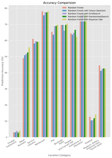
Figure 1. Accuracy Graph of Random Forest.

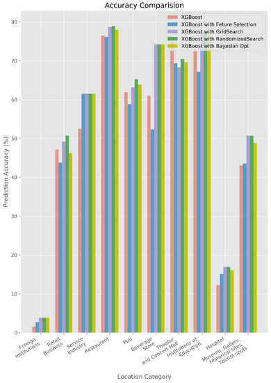
Figure 2. Accuracy Graph of XGBoost.

In addition, Figure 3 shows that Stacking with feature selection resulted in high prediction accuracy. Maybe aggregation of five different models of Stacking reduces noise of data. In case of foreign institutions and hospital which has very small number of visit, five different models may lead to low accuracy in level 1 of Stacking and the aggregated results lead to low accuracy. It is notable that several of BFF were always included in selected features. It is proven that personality is highly related with visiting places.

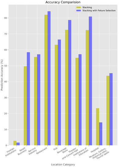
Figure 3. Accuracy Graph of Stacking.

Table 7 shows the results numerically: hyperparameter optimization and prediction accuracy. In Table 7, hyperparameter value of RF are chosen as n_estimators, max_depth, bootstrap, respectively and in case of XGB, n_estimators, max_depth, learning_rate, booster are shown. It is notable that feature selection leads to accuracy decrease however prediction accuracy can be increased with hyperparameter optimization. For most of Random Forest optimization, bootstrap is used for the most of location categories. Bootstrap is useful for smaller number of input data. In addition, different method of optimization for the same location categories leads to similar value of max_depth or n_estimators. Interestingly, different hyperparameters can lead to similar accuracy. Maybe the big structure generated in the leaning process by Random Forest and XGBoost enables convergence of accuracy. Especially, XGB is highly dependent on the selection of booster. It is important to select adequate booster for XGB. In addition, selection of number of iteration for bayesian optimization is also important. In case of theater and concert hall, low number of iteration for bayesian optimization leads to booster of ‘gblinear’. And the accuracy is reduced in 20% comparing to that of grid search or random search. Linear function of ’gblinear’ shows big gap in accuracy comparing to ‘gbtree’ and ‘dart’ which is based on tree structure. In addition, extra number of iteration leads to low prediction accuracy due to overfitting. We concluded that the number of iteration is in the range of 50 to 60.

Table 7. Optimized Hyperparameters.

Location Category	Optimization Algorithm	Learning Algorithm	Optimal Hyperparameter Values Searched	Accuracy (%) (100-SMAPE)
Foreign Institutions	Grid	RF	50, 15, True	3.98
		XGB	1000, 2, 0.3, ‘gblinear’	3.88
	Random	RF	250, 4, True	2.90
		XGB	1000, 5, 0.3, ‘gblinear’	3.88
	Bayesian	RF	150, 15, True	4.03
		XGB	1000, 15, 0.3, ‘gblinear’	3.88
Retail Business	Grid	RF	50, 9, True	51.67
		XGB	200, 2, 0.05, ‘gblinear’	49.20
	Random	RF	350, 9, True	52.57
		XGB	500, 12, 0.1, ‘gblinear’	50.78
	Bayesian	RF	450, 5, False	55.78
		XGB	350, 3, 0.3, ‘dart’	46.25
Service Industry	Grid	RF	250, 2, True	59.59
		XGB	50, 2, 0.1, ‘dart’	61.55
	Random	RF	950, 2, True	59.18
		XGB	550, 13, 0.1, ‘dart’	61.50
	Bayesian	RF	900, 2, True	59.09
		XGB	1000, 4, 0.05, ‘gbtree’	61.50
Restaurant	Grid	RF	50, 11, True	77.50
		XGB	50, 2, 0.05, ‘gblinear’	78.70
	Random	RF	200, 9, True	77.45
		XGB	650, 4, 0.05, ‘gblinear’	78.94
	Bayesian	RF	250, 5, True	77.95
		XGB	100, 10, 0.05, ‘gblinear’	78.76
Pub	Grid	RF	50, 3, True	68.83
		XGB	50, 2, 0.25, ‘gbtree’	63.19
	Random	RF	100, 2, True	69.09
		XGB	900, 7, 0.2, ‘gblinear’	65.30
	Bayesian	RF	250, 14, True	69.82
		XGB	900, 2, 0.25, ‘dart’	63.86
Beverage Store	Grid	RF	50, 12, True	66.02
		XGB	1000, 2, 0.3, ‘gblinear’	74.25
	Random	RF	50, 9, True	69.66
		XGB	800, 9, 0.3, ‘gblinear’	74.25
	Bayesian	RF	50, 10, True	70.40
		XGB	1000, 4, 0.3, ‘gblinear’	74.25
Theater and Concert Hall	Grid	RF	150, 6, True	64.76
		XGB	50, 2, 0.15, ‘dart’	68.32
	Random	RF	100, 13, True	66.60
		XGB	500, 5, 0.1, ‘gbtree’	70.49
	Bayesian	RF	950, 2, True	62.26
		XGB	733. 2. 0.15, ‘gbtree’	69.64
Institutions of Education	Grid	RF	50, 6, True	77.05
		XGB	1000, 5, 0.3, ‘gblinear’	77.45
	Random	RF	400, 3, True	76.20
		XGB	900, 12, 0.2, ‘gblinear’	77.45
	Bayesian	RF	100, 15, True	76.22
		XGB	944, 14, 0.55, ‘gblinear’	77.45
Hospital	Grid	RF	100, 10, True	10.62
		XGB	50, 5, 0.1, ‘gbtree’	16.97
	Random	RF	50, 15, True	11.84
		XGB	50, 13, 0.1, ‘gbtree’	16.97
	Bayesian	RF	100, 2, False	14.13
		XGB	293, 15, 0.55, ‘gblinear’	16.11
Museum, Gallery, Historical site, Tourist spots	Grid	RF	150, 2, True	42.38
		XGB	1000, 5, 0.3, ‘gblinear’	50.74
	Random	RF	1000, 2, True	42.68
		XGB	500, 9, 0.25, ‘gblinear’	50.72
	Bayesian	RF	700, 2, True	42.55
		XGB	76, 10, 0.2, ‘gblinear’	48.83

As predicted, execution time for three different optimization is quite different. Table 8 shows execution time with hyperparameter optimization. Figure 4 is for RF and Figure 5 is for XGB, respectively. Even though grid search and random search shows similar performance, however, there is big difference in execution time. In addition, bayesian optimization is a little bit slower than random search but quite faster than grid search. We guess bayesian search is the choice due to the balance of execution time and performance. As well, prior knowledge is reflected in bayesian optimization.

Table 8. Hyperparameter Optimization Execution Time.

Location Category	Optimization Algorithm	Learning Algorithm	Execution Time (in Seconds)
Foreign Institutions	Grid	RF	546.29
		XGB	259.12
	Random	RF	6.68
		XGB	4.50
	Bayesian	RF	190.65
		XGB	27.08
Retail Business	Grid	RF	542.62
		XGB	345.77
	Random	RF	8.33
		XGB	5.82
	Bayesian	RF	143.21
		XGB	18.48
Service Industry	Grid	RF	551.15
		XGB	198.99
	Random	RF	9.06
		XGB	0.91
	Bayesian	RF	135.79
		XGB	18.23
Restaurant	Grid	RF	557.60
		XGB	297.58
	Random	RF	5.39
		XGB	4.92
	Bayesian	RF	142.96
		XGB	23.84
Pub	Grid	RF	657.58
		XGB	284.47
	Random	RF	6.24
		XGB	4.85
	Bayesian	RF	289.76
		XGB	31.11
Beverage Store	Grid	RF	542.57
		XGB	292.10
	Random	RF	3.53
		XGB	1.03
	Bayesian	RF	148.80
		XGB	13.14
Theater and Concert Hall	Grid	RF	550.68
		XGB	211.76
	Random	RF	7.57
		XGB	5.22
	Bayesian	RF	152.43
		XGB	30.92
Institutions of Education	Grid	RF	571.96
		XGB	122.84
	Random	RF	7.88
		XGB	1.59
	Bayesian	RF	176.90
		XGB	36.61
Hospital	Grid	RF	326.95
		XGB	181.21
	Random	RF	5.54
		XGB	4.79
	Bayesian	RF	169.42
		XGB	29.93
Museum, Gallery, Historical site, Tourist spots	Grid	RF	558.27
		XGB	260.24
	Random	RF	7.54
		XGB	4.88
	Bayesian	RF	161.72
		XGB	22.67

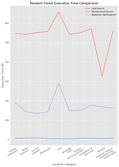
Figure 4. Execution Time Graph of Random Forest.

Figure 5. Execution Time Graph of XGBoost.

The total representation of accuracy of three different models can be found in Table 9, Table 10 and Table 11. Figure 1, Figure 2 and Figure 3 aforementioned shows the accuracy of each experimental condition. For the Stacking, hyperparameter optimization cannot be made due to the nature of Stacking, meta learning. Once hyperparameter optimization is applied to Stacking, every model in level 1 of Stacking must contain hyperparameter optimization which will result in drastic increase of execution time. Actually, Stacking with feature selection shows the prediction accuracy as high as RF and XGB with hyperparameter optimization. Figure 6 shows prediction accuracy for each location category. The cases of foreign institutions and hospital are somewhat incredible due to low accuracy, and due to smaller number of raw data. For other location categories, prediction accuracy is in the range of 50% to 80%. As aforementioned, too various subcategories shows somewhat low accuracy while ramification of subcategories could lead to higher prediction accuracy. For instance, distinct location categories such as restaurant, pub, beverage store, theater and concert hall show high accuracy.

Table 9. Accuracy of Random Forest.

	Learning Model	RF	+Feature Selection	+Hyperparameter Optimization
Location Category				Grid	Random	Bayesian
Foreign Institutions		2.96	3.07	3.98	2.9	4.03
Retail Business		48.98	50.89	51.67	52.57	55.78
Service Industry		60.98	58.16	59.59	59.18	59.09
Restaurant		78.09	75.6	77.5	77.45	77.95
Pub		65.32	63.62	68.83	69.09	69.82
Beverage Store		69.66	69.59	66.02	69.66	70.4
Theater and Concert Hall		64.43	63.62	64.76	66.6	62.26
Institutions of Education		76.66	75.79	77.05	76.2	76.22
Hospital		12.63	10.44	10.62	11.84	14.13
Museum, Gallery, Historical site, Tourist spots		44.57	41.18	42.38	42.68	42.55

Table 10. Accuracy of XGBoost.

	Learning Model	XGB	+Feature Selection	+Hyperparameter Optimization
Location Category				Grid	Random	Bayesian
Foreign Institutions		1.56	2.72	3.88	3.88	3.88
Retail Business		47.16	43.76	49.20	50.78	46.25
Service Industry		52.50	61.50	61.55	61.50	61.50
Restaurant		76.44	76.15	78.70	78.94	78.76
Pub		61.90	58.84	63.19	65.30	63.86
Beverage Store		60.97	52.30	74.25	74.25	74.25
Theater and Concert Hall		74.99	69.39	68.32	70.49	69.64
Institutions of Education		72.49	67.14	77.45	77.45	77.45
Hospital		12.30	15.15	16.97	16.97	16.11
Museum, Gallery, Historical site, Tourist spots		43.06	43.57	50.74	50.72	48.83

Table 11. Accuracy of Stacking.

	Learning Model	Stacking	+Feature Selection
Location Category
Foreign Institutions		2.88	1.77
Retail Business		49.65	58.50
Service Industry		55.51	57.19
Restaurant		82.03	84.19
Pub		63.20	66.43
Beverage Store		72.52	78.75
Theater and Concert Hall		55.01	57.25
Institutions of Education		72.40	80.90
Hospital		23.40	14.48
Museum, Gallery, Historical site, Tourist spots		43.76	45.35

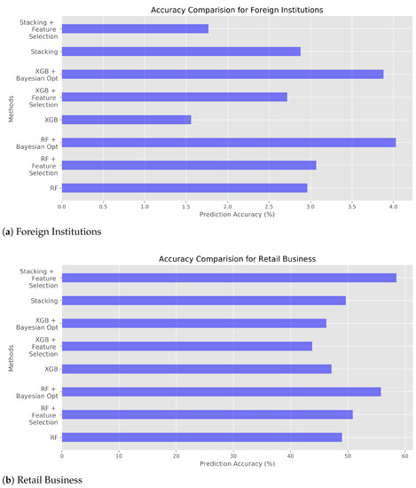
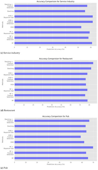
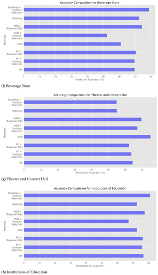
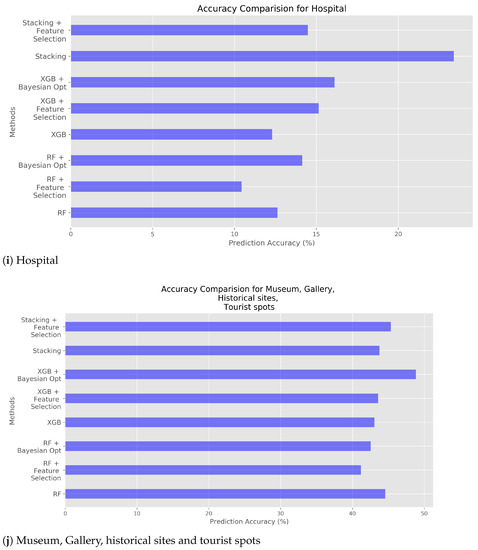
Figure 6. Predict Accuracy Comparison of all methods.

5. Conclusions and Future Works

Location Based Service (LBS) and recommendation system are typical examples of personalized service. For example, contents providers such as Netflix opened a competition for recommendation system development. However, recommendation systems have cold start problem which makes recommendation difficult for the new users or new contents. In addition, personal information protection of history is another sort of problem. It could be possible if we can predict user preference based on basic user features regardless of history. From various research, it is discussed that human personality and location preference is highly related. Additionally, personal features other than personality also related with preference of location visiting. Of course, there are meaningful, distinguished personal features for personal location preference.

In this research, from three different methods of machine learning, we figured out the effects of distinguished personal features for personal location preference. As a result, eight location categories out of ten showed meaningful prediction accuracy: Retail Business, Service industry, Restaurant, Pub, Beverage Store, Theater and Concert Hall, Institutions of Education, and Museum, Gallery, Historical sites, Tourist spots. For each of three algorithms, prediction accuracy seem to be reliable with very similar tendency of analysis results. As well, input features were selected which affects location category selection with Random Forest and XGBoost, and of course, input features are dependent on location categories. Based on our research, visiting preference to such location categories can be highly predictable from personal features. In addition, hyperparameter optimization which is a sort of AutoML technology is introduced in order to increase prediction accuracy. Grid search, random search as well as bayesian optimization are applied and the results are compared.

In our research, we demonstrated a method for visiting place prediction. For large amount of input data, feature selection is applied in order to reduce dimension of data and increase quality of input data. In such cases, Stacking could be one of the best solution even without hyperparameter optimization. On the contrary, for smaller number of input data, bagging or boosting in addition with hyperparameter optimization could be a better solution since Stacking may show poor prediction accuracy. We need to research further, especially for location categories such as service industry, retail business since too many subcategories make the categorization vague. In addition, less sensitive personal features must exists for the prediction of visiting location. Such features will be able to be identified. From the aspect of volunteers’ data, we need to expand data collection for more number of data as well as wider span of data, since our data is clear limitations of volunteer pool; engineering students in his or her twenties.

References

- Song, H.Y.; Lee, E.B. An analysis of the relationship between human personality and favored location. In Proceedings of the AFIN 2015, The Seventh International Conference on Advances in Future Internet, Venice, Italy, 23–28 August 2015; p. 12. [Google Scholar]
- Song, H.Y.; Kang, H.B. Analysis of Relationship Between Personality and Favorite Places with Poisson Regression Analysis. ITM Web Conf. 2018, 16, 02001. [Google Scholar] [CrossRef][Green Version]
- Kim, S.Y.; Song, H.Y. Determination coefficient analysis between personality and location using regression. In Proceedings of the International Conference on Sciences, Engineering and Technology Innovations, ICSETI, Bali, India, 22 May 2015; pp. 265–274. [Google Scholar]
- Kim, S.Y.; Song, H.Y. Predicting Human Location Based on Human Personality. In International Conference on Next Generation Wired/Wireless Networking, Proceedings of the NEW2AN 2014: Internet of Things, Smart Spaces, and Next Generation Networks and Systems, St. Petersburg, Russia, 27–29 August 2014; Lecture Notes in Computer Science; Springer International Publishing: Cham, Switzerland, 2014; pp. 70–81. [Google Scholar] [CrossRef]
- Kim, Y.M.; Song, H.Y. Analysis of Relationship between Personal Factors and Visiting Places using Random Forest Technique. In Proceedings of the Federated Conference on Computer Science and Information Systems (FedCSIS), Leipzig, Germany, 1–4 September 2019; pp. 725–732. [Google Scholar]
- Song, H.Y.; Yun, J. Analysis of the Correlation Between Personal Factors and Visiting Locations With Boosting Technique. In Proceedings of the Federated Conference on Computer Science and Information Systems (FedCSIS), Leipzig, Germany, 1–4 September 2019; pp. 743–746. [Google Scholar]
- Li, J.; Cheng, K.; Wang, S.; Morstatter, F.; Trevino, R.P.; Tang, J.; Liu, H. Feature selection: A data perspective. ACM Comput. Surv. (CSUR) 2017, 50, 1–45. [Google Scholar] [CrossRef]
- Shahriari, B.; Swersky, K.; Wang, Z.; Adams, R.P.; De Freitas, N. Taking the human out of the loop: A review of Bayesian optimization. Proc. IEEE 2015, 104, 148–175. [Google Scholar] [CrossRef]
- Snoek, J.; Larochelle, H.; Adams, R.P. Practical bayesian optimization of machine learning algorithms. arXiv 2012, arXiv:1206.2944. [Google Scholar]
- Zhou, Z.H. Ensemble Methods: Foundations and Algorithms; Chapman and Hall/CRC: Boca Raton, FL, USA, 2012. [Google Scholar]
- Bennett, J.; Lanning, S. The netflix prize. In Proceedings of the KDD Cup and Workshop; Citeseer: New York, NY, USA, 2007; Volume 2007, p. 35. [Google Scholar]
- Breiman, L. Random forests. Mach. Learn. 2001, 45, 5–32. [Google Scholar] [CrossRef]
- Segal, M.R. Machine Learning Benchmarks and Random Forest Regression. UCSF: Center for Bioinformatics and Molecular Biostatistics. 2004. Available online: https://escholarship.org/uc/item/35x3v9t4 (accessed on 27 June 2021).
- Chen, T.; Guestrin, C. Xgboost: A scalable tree boosting system. In Proceedings of the 22nd ACM Sigkdd International Conference on Knowledge Discovery and Data Mining, San Francisco, CA, USA, 13–17 August 2016; pp. 785–794. [Google Scholar]
- Wolpert, D.H. Stacked generalization. Neural Netw. 1992, 5, 241–259. [Google Scholar] [CrossRef]
- Géron, A. Hands-On Machine Learning with Scikit-Learn, Keras, and TensorFlow: Concepts, Tools, and Techniques to Build Intelligent Systems; O’Reilly Media: Newton, MA, USA, 2019. [Google Scholar]
- Costa, P.T.; McCrae, R.R. Four ways five factors are basic. Personal. Individ. Differ. 1992, 13, 653–665. [Google Scholar] [CrossRef]
- Hoseinifar, J.; Siedkalan, M.M.; Zirak, S.R.; Nowrozi, M.; Shaker, A.; Meamar, E.; Ghaderi, E. An Investigation of The Relation Between Creativity and Five Factors of Personality In Students. Procedia Soc. Behav. Sci. 2011, 30, 2037–2041. [Google Scholar] [CrossRef]
- Jani, D.; Jang, J.H.; Hwang, Y.H. Big five factors of personality and tourists’ Internet search behavior. Asia Pac. J. Tour. Res. 2014, 19, 600–615. [Google Scholar] [CrossRef]
- Jani, D.; Han, H. Personality, social comparison, consumption emotions, satisfaction, and behavioral intentions. Int. J. Contemp. Hosp. Manag. 2013, 25, 970–993. [Google Scholar] [CrossRef]
- John, O.P.; Srivastava, S. The Big Five trait taxonomy: History, measurement, and theoretical perspectives. In Handbook of Personality: Theory and Research; University of California: Berkeley, CA, USA, 1999; Volume 2, pp. 102–138. [Google Scholar]
- Amichai-Hamburger, Y.; Vinitzky, G. Social network use and personality. Comput. Hum. Behav. 2010, 26, 1289–1295. [Google Scholar] [CrossRef]
- Chorley, M.J.; Whitaker, R.M.; Allen, S.M. Personality and location-based social networks. Comput. Hum. Behav. 2015, 46, 45–56. [Google Scholar] [CrossRef]
- Foursquare Labs, Inc. Swarm App. 2019. Available online: https://www.swarmapp.com/ (accessed on 27 June 2021).
- Armstrong, J.S. Long-Range Forecasting; Wiley New York ETC.: New York, NY, USA, 1985. [Google Scholar]
- Flores, B.E. A pragmatic view of accuracy measurement in forecasting. Omega 1986, 14, 93–98. [Google Scholar] [CrossRef]
- Tofallis, C. A better measure of relative prediction accuracy for model selection and model estimation. J. Oper. Res. Soc. 2015, 66, 1352–1362. [Google Scholar] [CrossRef]
Publisher’s Note: MDPI stays neutral with regard to jurisdictional claims in published maps and institutional affiliations. |
© 2021 by the authors. Licensee MDPI, Basel, Switzerland. This article is an open access article distributed under the terms and conditions of the Creative Commons Attribution (CC BY) license (https://creativecommons.org/licenses/by/4.0/).