Autonomous Mobile Robot Navigation in Sparse LiDAR Feature Environments

Abstract

In the industrial environment, Autonomous Guided Vehicles (AGVs) generally run on a planned route. Among trajectory-tracking algorithms for unmanned vehicles, the Pure Pursuit (PP) algorithm is prevalent in many real-world applications because of its simple and easy implementation. However, it is challenging to decelerate the AGV’s moving speed when turning on a large curve path. Moreover, this paper addresses the kidnapped-robot problem occurring in spare LiDAR environments. This paper proposes an improved Pure Pursuit algorithm so that the AGV can predict the trajectory and decelerate for turning, thus increasing the accuracy of the path tracking. To solve the kidnapped-robot problem, we use a learning-based classifier to detect the repetitive pattern scenario (e.g., long corridor) regarding 2D LiDAR features for switching the localization system between Simultaneous Localization And Mapping (SLAM) method and Odometer method. As experimental results in practice, the improved Pure Pursuit algorithm can reduce the tracking error while performing more efficiently. Moreover, the learning-based localization selection strategy helps the robot navigation task achieve stable performance, with 36.25% in completion rate more than only using SLAM. The results demonstrate that the proposed method is feasible and reliable in actual conditions.

1. Introduction

In recent years, due to the dramatic development and evolution of technology, an increasing number of industries have turned to automation. The AGV plays a significant role in the automation and is widely used in various other fields.

1.1. Path Planning and Trajectory-Tracking Algorithms

In unmanned vehicle navigation, path planning is essential to search for an optimal path from one point to another point in the environment. Researchers have adopted different methods to solve the problem of AGV path planning, two of which are grid search-based methods and intelligent-based methods. Grid Search-based methods include the A* algorithm and its variants. Chang et al. [1] proposed an improved A* path planning algorithm based on a compressed map to reveal actual narrow areas the robot cannot reach although this approach produces some precision loss, leading the path to be conservative. To reduce the redundant points in A* algorithm pathfinding process, Zeng et al. [2] used Jump Point Search to obtain jump points in the raster map and speed up the A* algorithm based on obtained jump points, though the search time fluctuates in different practical scenarios. For intelligent-based methods, Huang et al. [3] proposed an improved genetic algorithm under a global static environment, which improved the slow convergence and precocity problems. Meanwhile, Zhang et al. [4] refined inertia weights and acceleration factors in Particle Swarm Optimization to prevent local minimum value falling and increase convergence speed.

Following path planning process, trajectory tracking is required so that the AGV can track the movement according to a set trajectory path. With the development of technology, various trajectory-tracking methods have been proposed. Wu et al. [5] introduced a local linear Model Predictive Control (MPC) to track the nonlinear vehicle model velocity and path simultaneously. In [6], a reference trajectory is predefined using a sigmoid function. Then the trajectory is adjusted dynamically by a nonlinear MPC when an obstacle appears in the predictive horizon. Besides MPC, Yang et al. [7] proposed a Fixed-Time Control method and a Fixed-Time Sliding Mode Controller to trajectory-tracking control while meeting the predetermined performance and disturbance suppression. Furthermore, an adaptive trajectory-following strategy was proposed in [8] that constructs a knowledge database through the Particle Swarm Optimization (PSO) algorithm to optimize the controller parameters set according to various vehicle speed and heading error combinations. Meanwhile, Yan et al. [9] proposed a hybrid visual trajectory strategy in which a 2.5D visual servo framework was used to enhance trajectory-tracking behavior.

Although non-geometric controllers such as MPC can be applied to linear or nonlinear models with multiple constraints, their limitations are heavy computation and an inability to provide a closed-form solution when the model is sophisticated. On the other hand, the Pure Pursuit (PP) algorithm is a popular trajectory-tracking algorithm because of its simplicity, efficiency, and low computational requirements, even in limited resource conditions. It computes angular velocity to move the robot from its current position to some look-ahead point in front of the robot. However, the tracking performance is poor due to improper selection of the look-ahead distance. Chen et al. [10] combined the PP algorithm with Proportional Integral (PI) Controller to smooth the final output steering angle through a low-pass filter and verify its feasibility through simulation experiments. By analyzing the vehicle speed and the shortest distance between the GPS trajectory and the current vehicle position, Wang et al. [11] proposed an algorithm that can reduce the lateral error when the vehicle tracks the ideal path. Meanwhile, a Pure Pursuit algorithm based on the optimized look-ahead distance (OLDPPA) [12] introduced an adaptive random motion mechanism of particles in the Salp Swarm Algorithm to improve mining and exploration capabilities.

1.2. AGV Localization Algorithms

To navigate autonomously and safely, the AGV needs to be able to locate its position in its environment. Consequently, the localization problem has been studied and various techniques are proposed to solve the localization problem [13]. The simple form for localization is to use odometry methods, which provide the current position from odometry information estimated by velocity and rotation of wheels (wheel odometry), inertial measurement units (IMU odometry), laser source (laser odometry) or images (visual odometry), etc. For instance, a free-sensor LiDAR-based odometry method [14] integrated the LiDAR-only odometry (LOAM) algorithm to estimate odometry then segment the local map by Convolutional Neural Network (CNN) before using a two-stage RANSAC for verifying the position matches in the local map. Moreover, Zhao et al. [15] proposed a multi-model sensor fusion framework that uses different tightly coupled and loosely coupled optimization methods around the primary IMU odometry factors and can work in several challenging environments.

In contrast, the Simultaneous Localization And Mapping (SLAM) technology consists of the map building process and the localization process. In [16], the authors enhanced the localization method using least square-based geometric matching to compensate for the predicted position. Using 2D LiDAR scan, Millance et al. [17] use a Determinant of Hessian-based detector to find points of high curvature on the Signed Distance Function (SDF) for place recognition. Although the LiDAR-based SLAM method provides helpful information to determine free-space regions and characterizes places for localization, it seems inefficient in structure-less environments, e.g., long corridors, tunnels, dusty or foggy areas, etc. On the other hand, the Sensor-based odometry method proves their accuracy and robustness in various scenarios, even in challenging environments.

Currently, modern image classification systems based on deep neural networks, including Inception V3 [18] and YOLO V3 [19], are more accurate than traditional machine learning classification methods. In general, mobile robots are usually equipped with LiDAR for robot localization due to its accuracy, speed, and 3D reconstruction ability. Therefore, a deep neural network can extract the features of the LiDAR point-cloud data. For example, Chen et al. [20] extracted 2D LiDAR features and used SVM to recognize front pedestrians and track them. However, in the repetitive pattern environment, e.g., in the long corridor, where LiDAR point clouds are sparse to collect. As the result, it is challenging to localize precisely the AGV position, leading to mislocalization or the kidnapped-robot problem. When a mobile robot fails to localize itself due to sparse LiDAR point-cloud, some methods are developed to relocate AGV’s position. In the SLAM localization system, it localizes AGV’s position through Monte Carlo Localization (MCL) method, which takes a long time and is not helpful in broad-space scenarios. Therefore, Wi-Fi fingerprinting was proposed to solve the problem of robot kidnapping [21], and MCL was integrated with the Fast Library for Approximate Nearest Neighbors (FLANN) machine learning technology to solve this problem [22].

1.3. Contributions

Motivated by discussion above, this paper focused on control movement ability of the AGV on curve path and localizing the AGV on the localization system in the structure-less environment (long corridor). The main contributions of our work are as follows:

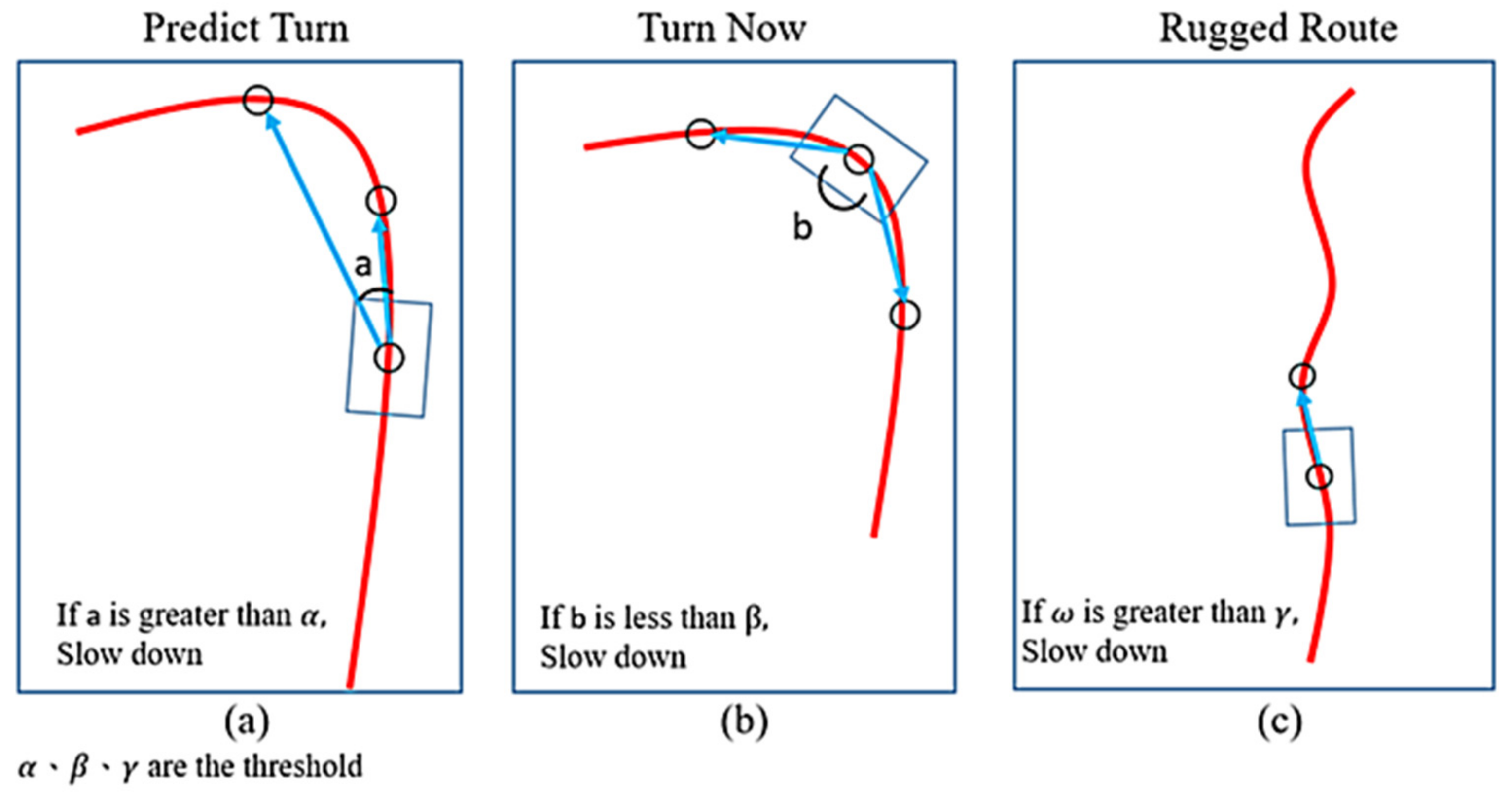
• For trajectory tracking, we adopt the PP algorithm and improves it. The traditional PP algorithm often causes errors when it encounters a turn because it is overdue to decelerate speed. Therefore, an improved PP algorithm is proposed that incorporates turning prediction-based deceleration to reduce the impact caused by late attempts at deceleration.
• To solve the kidnapped-robot problem, we combine 2D LiDAR point-cloud features with a deep convolutional network-based classifier to distinguish the current situation for selecting SLAM or odometry localization system. Thus, if the AGV is in a situation where SLAM fails to determine robot position, the task can still be continued.
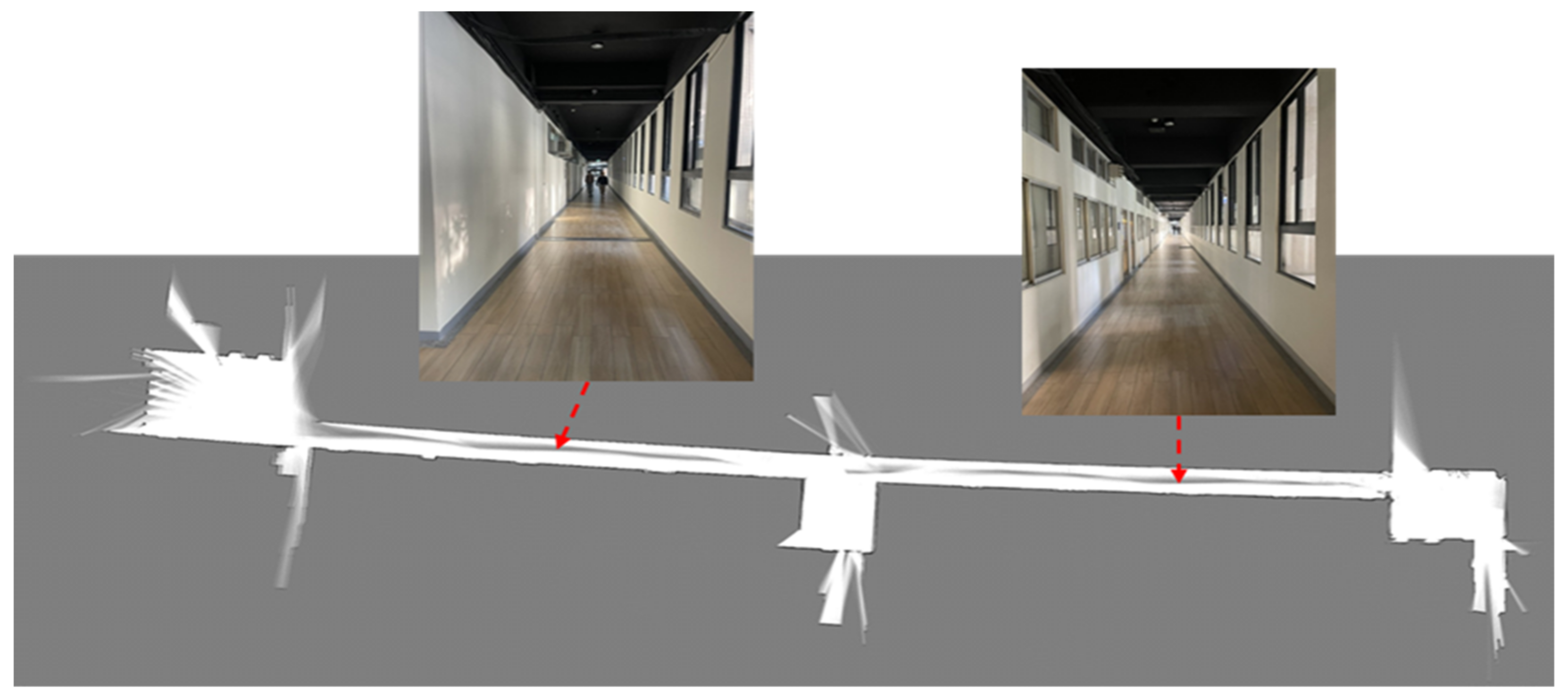
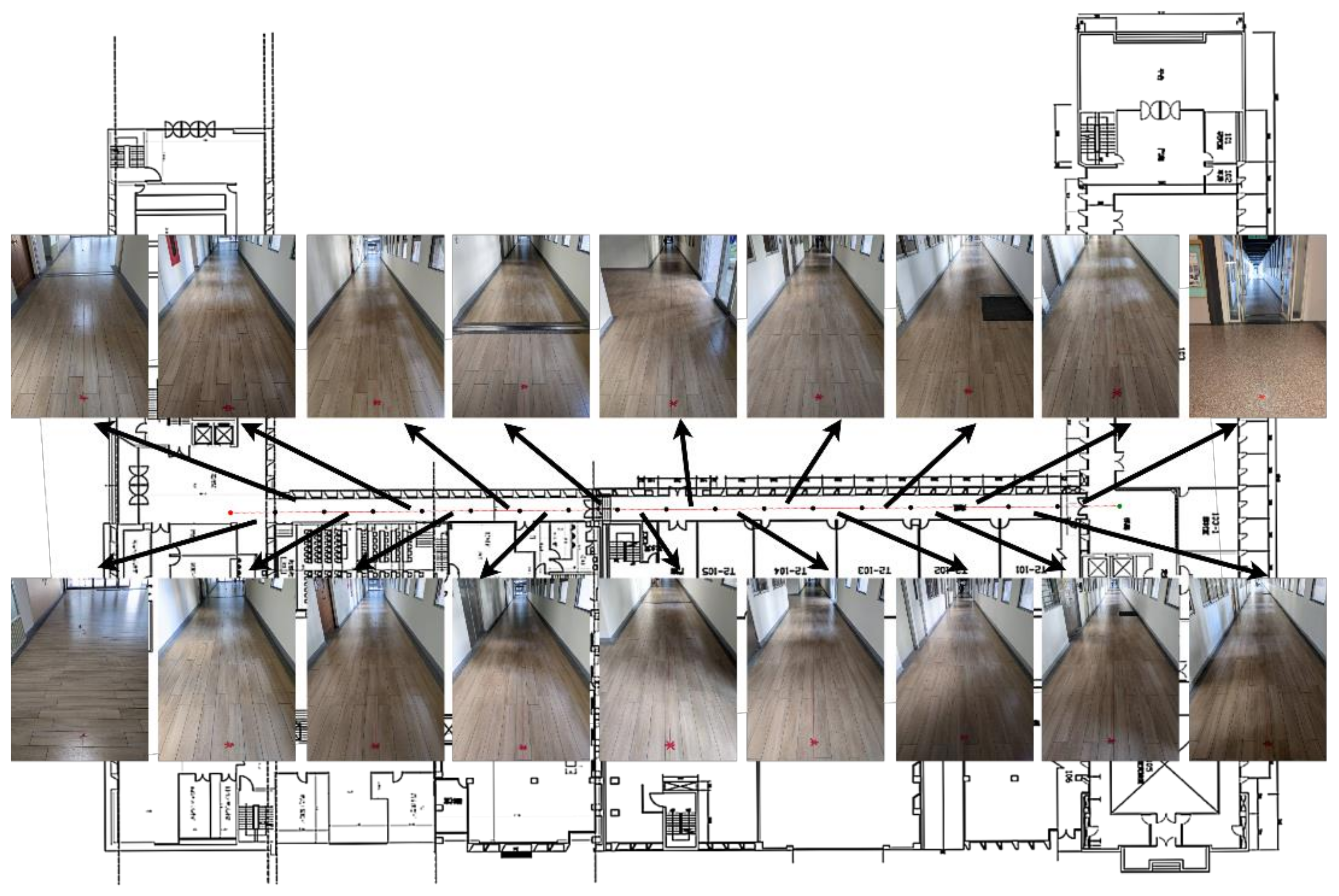
• In addition, practical experiments in the long corridor terrain are carried out to verify the feasibility of the proposed system.

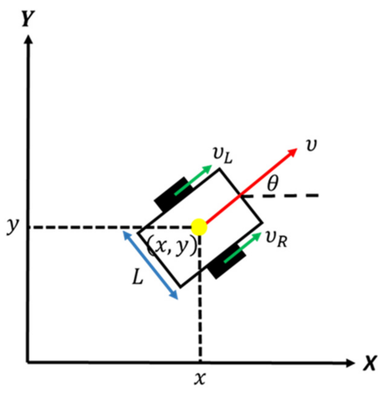
The remain of this paper is organized as follows. In Section 2, the hardware platform and vehicle kinematic of robot system are described. In Section 3, the improved Pure Pursuit algorithm using turning prediction-based speed adjustment is introduced. the deep learning-based selection strategy using 2D LiDAR point-cloud features for localization task is discussed Section 4. In Section 5, the practical experimental results and verification of the proposed method is reported. Finally, in Section 6, the conclusions are presented.

2. Robot System

The mobile robot has four differential wheels that use two motors on both left and right sides. In addition, the hardware platform is equipped with two LiDAR systems that can obtain 360-degree point-cloud information in the front and back of the robot for SLAM [23]. The schematic diagram of our mobile robot hardware platform is shown in Figure 1.

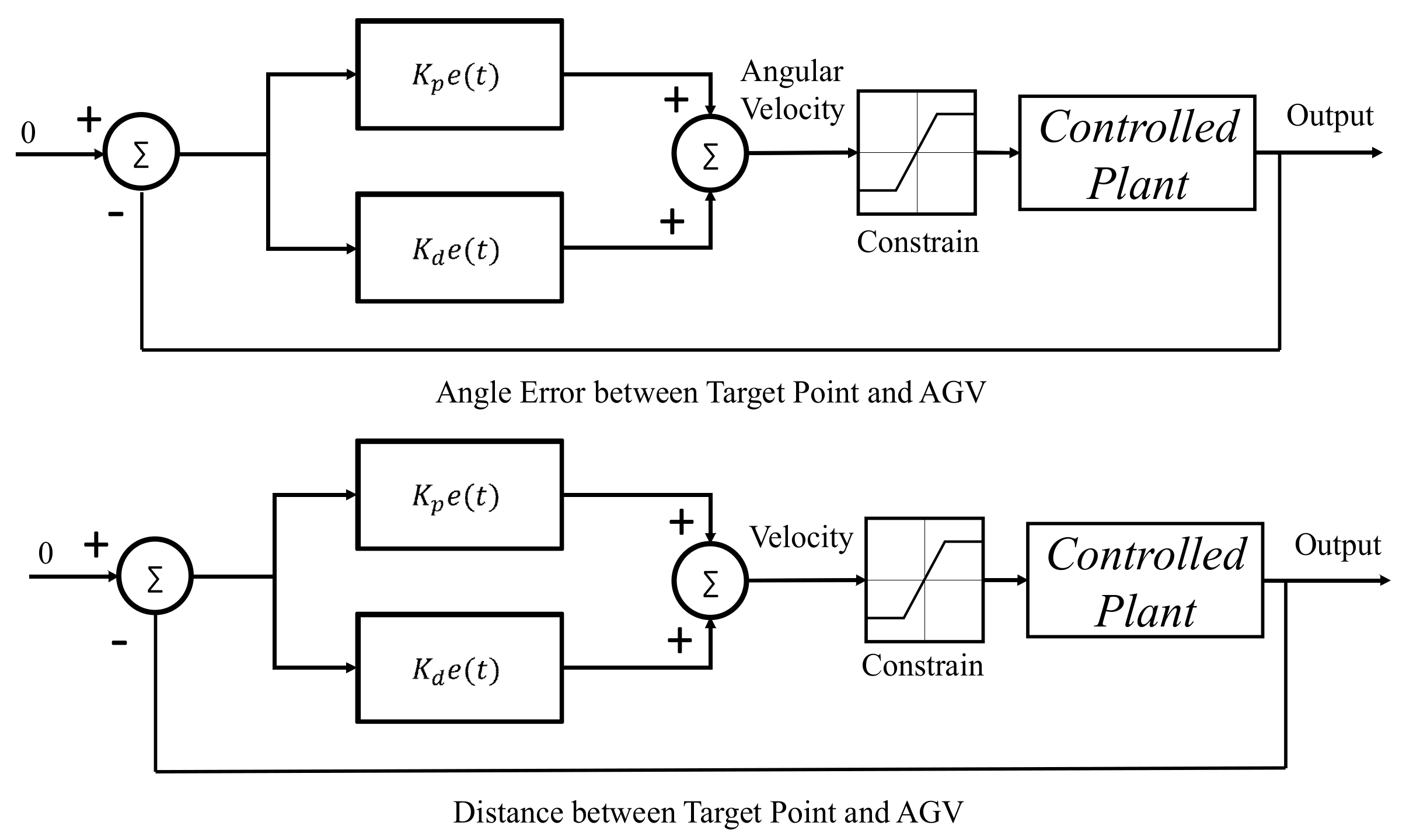
3. Design of Trajectory-Tracking System

The mobile robot in this paper is driven in a differential-wheel mode. The left and right wheels are related to the overall velocity and angular velocity of the mobile robot. The coordinate system of the mobile robot is shown in Figure 2, where $\left(x,y\right)$ is the location of the mobile robot, L is the distance between the left and right wheels, $\theta$ is the angle between the mobile robot and the X-axis, ${\upsilon }_R$ is the velocity of the right wheel, ${\upsilon }_L$ is the velocity of the left wheel, $\upsilon$ is the velocity of the mobile robot and $\omega$ is the angular velocity of the mobile robot. The kinematic model of the differential wheel is as follows:

$$x=\upsilon \cos \theta$$

(1)

$$y=\upsilon \cos \theta$$

(2)

$$\omega =\frac{{\upsilon }_R-{\upsilon }_L}{L}$$

(3)

$$\upsilon =\frac{{\upsilon }_R+{\upsilon }_L}{2}$$

(4)

$${\upsilon }_L=\upsilon -\frac{L\omega }{2}$$

(5)

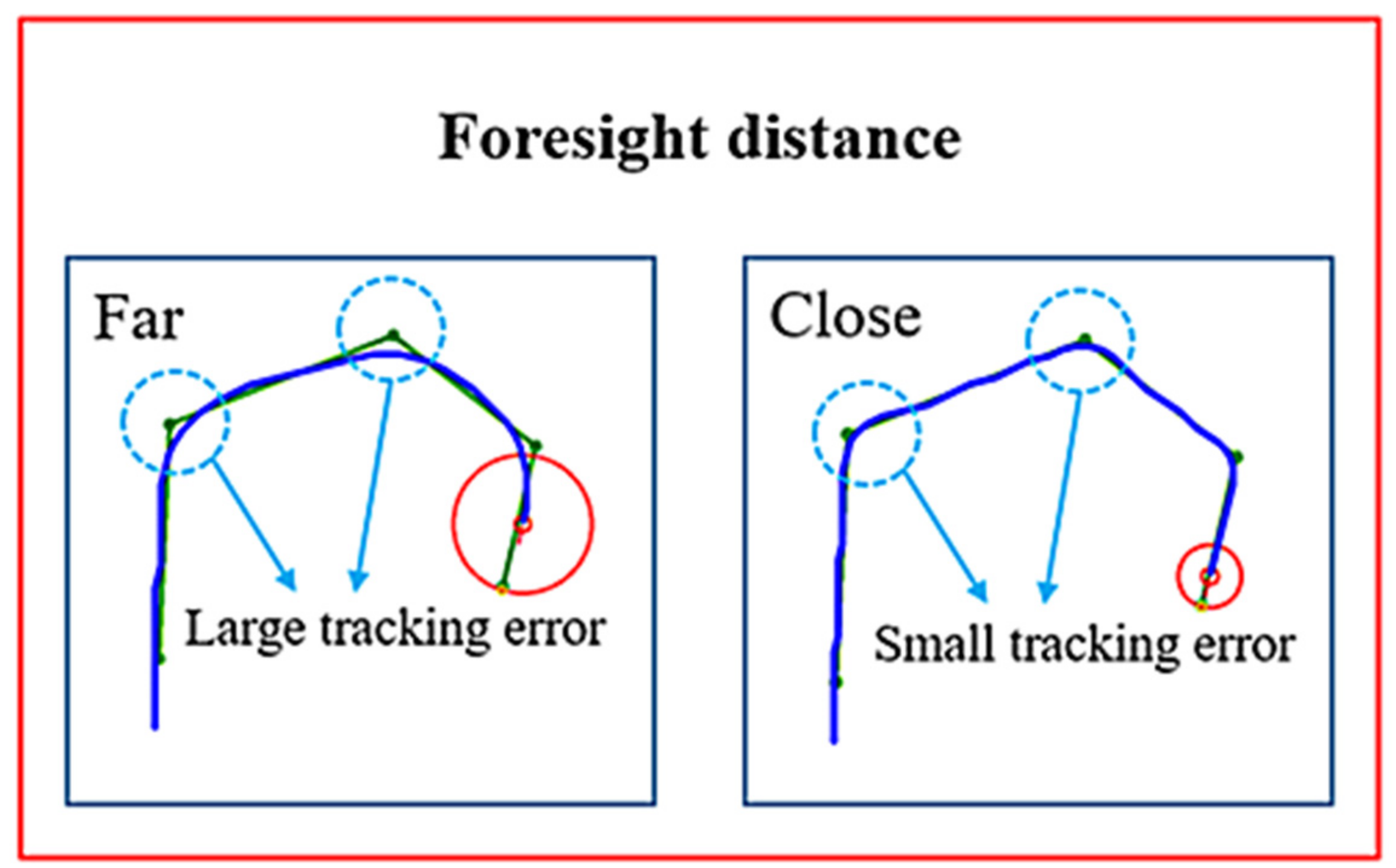
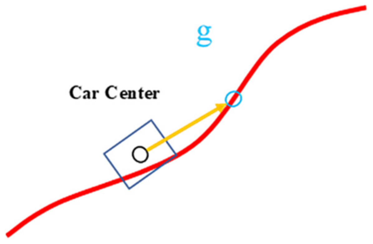
3.1. Introduction of Pure Pursuit (PP) Algorithm

In the PP algorithm, the target point g in tracking path is the target point between the forward-looking distance of the center of the vehicle body and the path. As shown in Figure 3, the target point g belongs to one of the points along the entire travel path. The forward-looking distance $L_f$ is calculated using Equation (6):

$$L_f=k_f\ast \upsilon +L_{fm}$$

(6)

where $k_f$ is the custom speed weight, $\upsilon$ is the linear velocity of the mobile robot and $L_{fm}$ is the minimum forward-looking distance limit.

The algorithm uses the PD controller to follow the path calculates the angle deviation according to the current position of the robot and the forward-looking distance point g, and then keeps the robot moving on the trajectory through the PD controller. The control structure block diagram of the PD controller is shown in Figure 4. In the PP algorithm, the forward-looking distance can impact to path tracking accuracy and may cause the mobile robot to oscillate, shown in Figure 5.

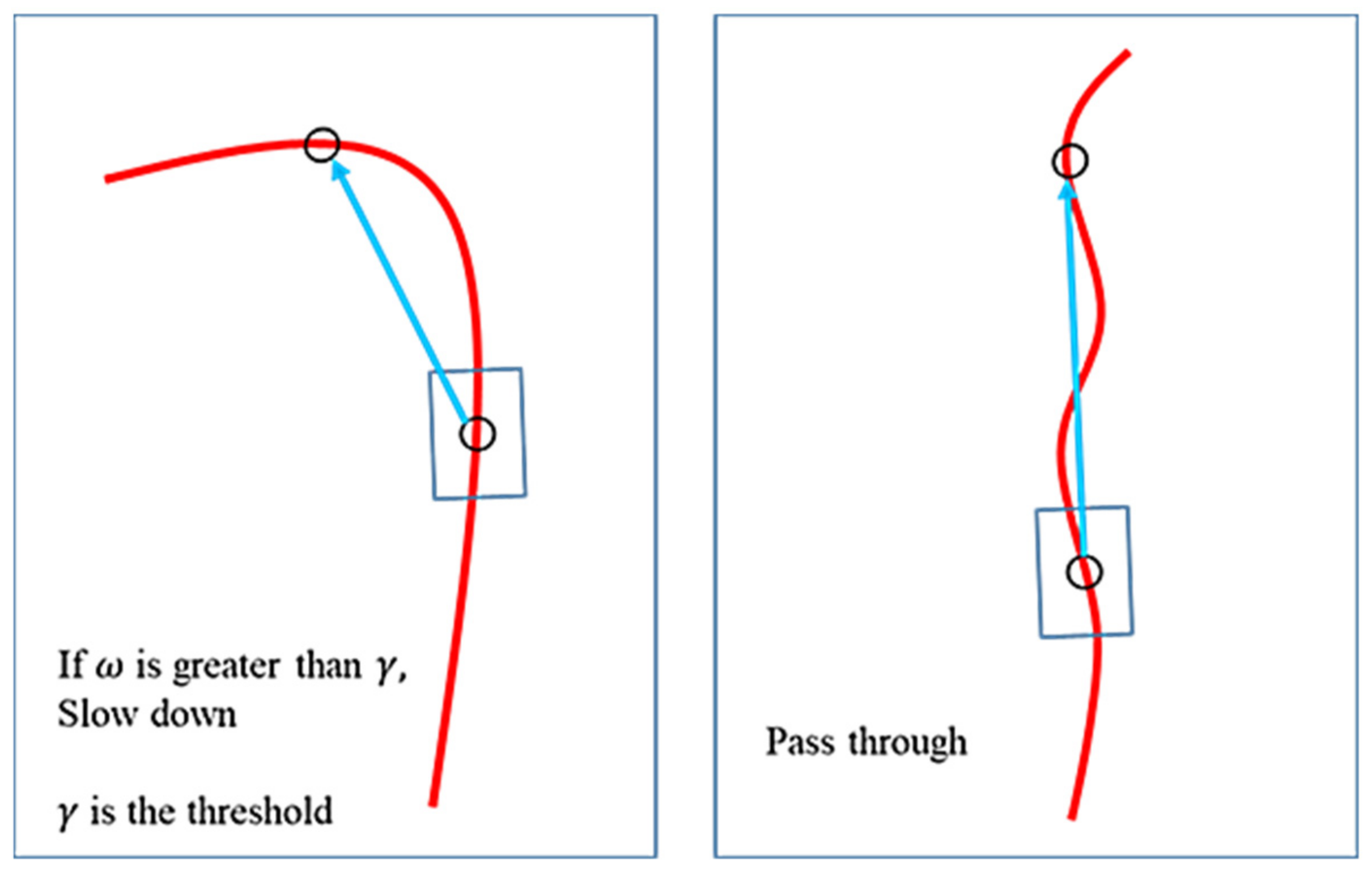
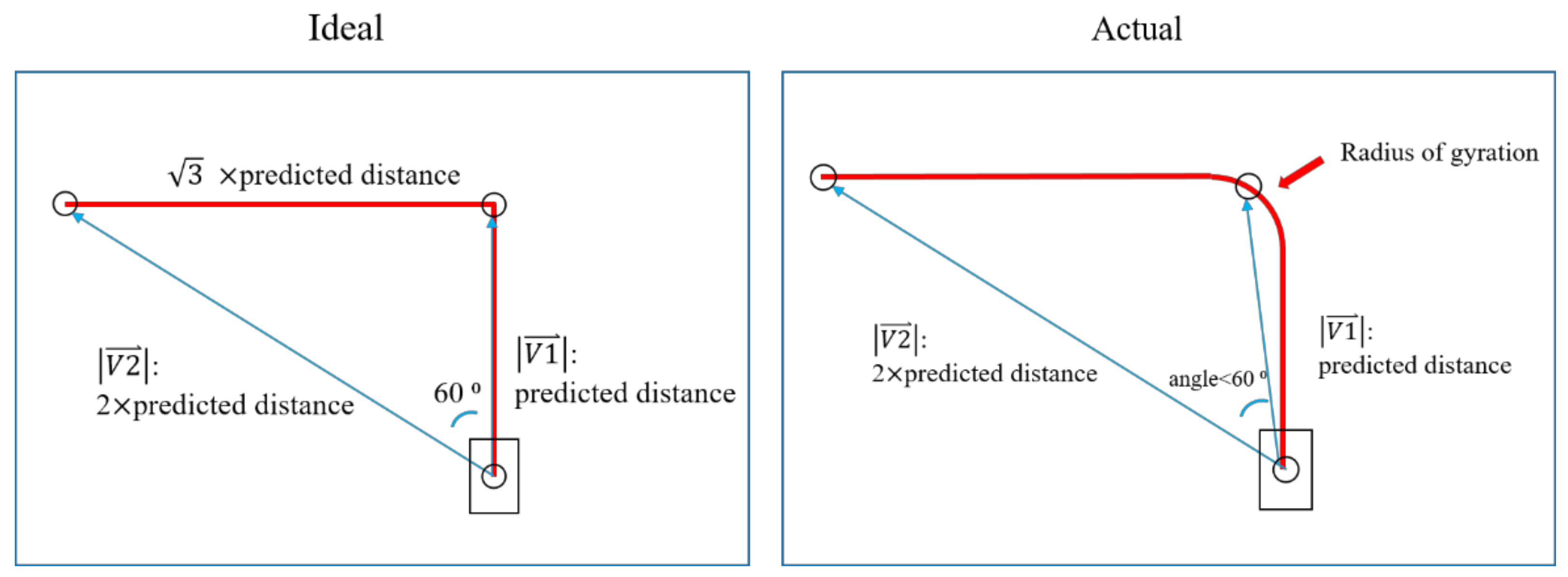
3.2. Improved Pure Pursuit Algorithm

In the original Pure Pursuit algorithm, the shorter the forward-looking distance, the higher the trajectory-tracking accuracy. As Equation (6) is adopted, the forward-looking distance $L_f$ is longer when the velocity $\upsilon$ is high; by contrast, $L_f$ is shorter when $\upsilon$ is slow. This leads that the turning time can be predicted when the angular velocity $\omega$ is large. However, the long forward-looking distance decreases trajectory-tracking accuracy, making it impossible to slow down the turn in time (Figure 6).

To improve the PP algorithm, this paper adopts a fixed short forward-looking distance to increase the trajectory-tracking ability at any time. Then the proposed method judges the current turn to decelerate it and keeps the angular velocity $\omega$ as a deceleration basis at a certain level so that the mobile robot can better track the path when the path is more rugged, shown in Figure 7.

We separate the turning decision strategy into three steps. First, we predict the turning distance using an angle $a$ between two vectors created from the current robot center to the two next forward-look points (shown in Figure 7a). Assume that two vectors $\left|\stackrel{\rightharpoonup }{V1}\right|$,$\left|\stackrel{\rightharpoonup }{V2}\right|$ of angle $a$ in the ideal situation (shown in Figure 8) as the following definition:

$$\left|\stackrel{\rightharpoonup }{V2}\right|\hspace{0.17em}=2\times \left|\stackrel{\rightharpoonup }{V1}\right|$$

(7)

where $\left|\stackrel{\rightharpoonup }{V1}\right|$ is the predicted distance, and the ideal angle $\alpha$ is ${60}^{°}$. When the ideal situation is encountered, the AGV will decelerate. However, when the route has a radius of gyration $R$, the angle $a$ will never reach $\alpha$ value and the AGV cannot decelerate. Without considering $R$, the maximum value of $\alpha$ can be obtained from $\left|\stackrel{\rightharpoonup }{V1}\right|$ and $\left|\stackrel{\rightharpoonup }{V2}\right|$ as below:

$$\alpha \le {\cos }^{-1}\left(\frac{\left|\stackrel{\rightharpoonup }{V2}\right|}{\left|\stackrel{\rightharpoonup }{V1}\right|}\right)$$

(8)

From Equation (8), we can clearly define the predicted turning distance with the corresponding radius of gyration R:

$${\cos }^{-1}\left(\frac{\left|\stackrel{\rightharpoonup }{V2}\right|}{\left|\stackrel{\rightharpoonup }{V1}\right|}\right)>{\tan }^{-1}\left(\frac{R}{\left|\stackrel{\rightharpoonup }{V1}\right|}\right)$$

(9)

$$\alpha \le {\cos }^{-1}\left(\frac{\left|\stackrel{\rightharpoonup }{V2}\right|}{\left|\stackrel{\rightharpoonup }{V1}\right|}\right)-{\tan }^{-1}\left(\frac{R}{\left|\stackrel{\rightharpoonup }{V1}\right|}\right)$$

(10)

In the following step (shown in Figure 7b), to make a turn action, we define a current turning angle $b$ between two vectors created from the current robot center to the next and the previous forward-looking points and ensure $b\le \beta$ value, where $\beta ={135}^{°}$ in ideal case. When the vehicle is traveling on rugged terrain (shown in Figure 7c), this paper uses $\gamma =0.1$ (rad/s) as the threshold to indicate that the angular velocity $\omega$ is too high if exceeding $\mathsf{\gamma }$, helping the mobile robot can increase the tracking accuracy.

4. The Localization Switching Method in the Structure-Less Environment

4.1. Two-Dimensional (2D) LiDAR SLAM

2D LiDAR SLAM technology uses LiDAR sensors to collect point-cloud data and scan matches. The SLAM technology then uses algorithms to optimize and loop closure detection for map building (Figure 9) and localization. However, in a structure-less environment as a long corridor, SLAM cannot determine its position on the map, leading to cause unexpected accidents easily. To avoid the mislocalization problem, we use the characteristics of 2D LiDAR data to recognize where the mobile robot is lost.

In scan matching, SLAM will match the point clouds with the map features. If the localization is successful, the point clouds are superimposed on the black edge of the SLAM map. At this time, we can use all point clouds and the point clouds superimposed on the black edge of the map to determine whether the AGV is mislocalized as follows:

$$m_r=1-\frac{p_{match}}{p_{all}}$$

(11)

where $m_r$ represents the missing rate (ranged from 0 to 1). If $m_r$ is greater than 50%, most of the point clouds are not superimposed on the map features. In this case, it can be judged that the mobile robot is getting lost; otherwise, it represents localization success. $p_{all}$ represents the number of all point clouds in a frame, and $p_{match}$ represents the number of point clouds in a frame superimposed on the map features.

However, this judgment method cannot detect the localization status under all conditions. when the surrounding environment has s repetitive pattern, the map features will be too consistent despite the point-cloud is superimposed on the map features. This makes SLAM localization impossible to confirm. For example, in the corridor part of the map (Figure 9), the point clouds extracted from the walls on both sides are too sparse, making it impossible to determine where the mobile robot is in the corridor.

4.2. Deep Learning-Based Corridor Recognition for Switching Localization Systems

To avoid the corridor effect, this paper proposes to use deep learning to identify where is corridor area to switch the localization system. Because we need to know whether the current environment belong to corridor area or not, we will define the corridor recognition problem as the binary classification problem. The process will be following as below:

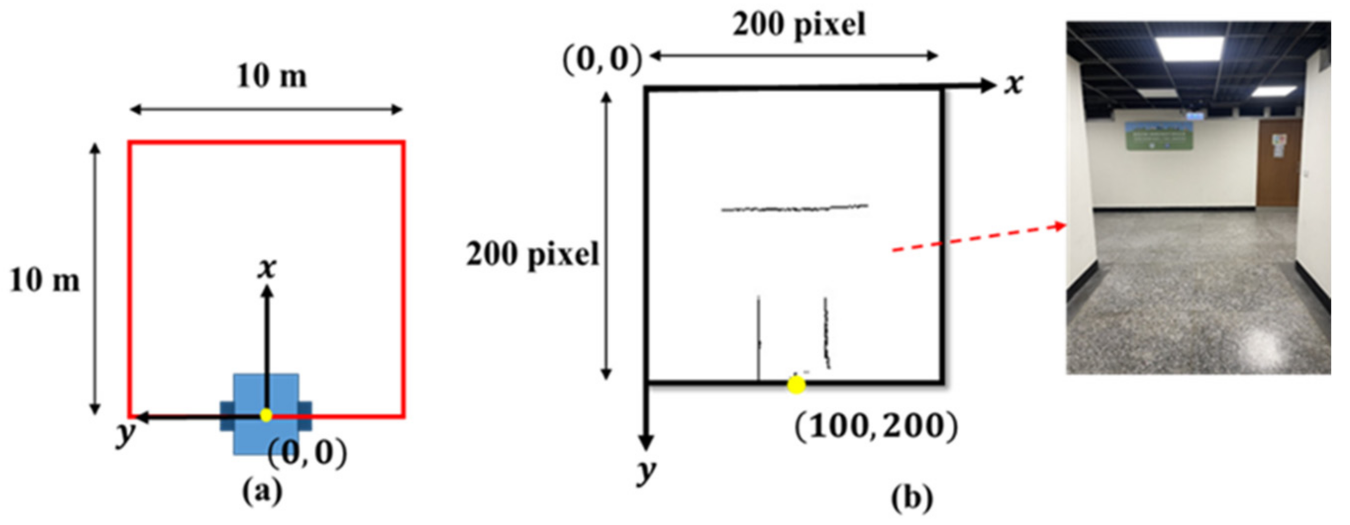
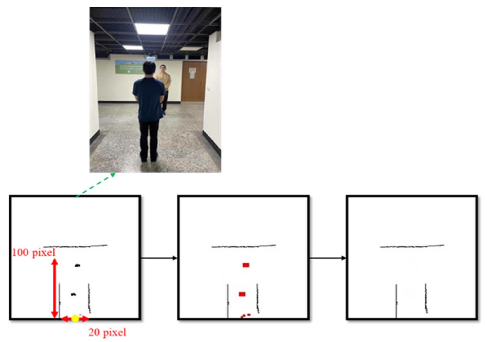
• First, to collect images that represent the current area, we need to convert the LiDAR point-cloud data into 2D images by the following formula:

  $$p_{pic}=\underset{R_{pic}}{r\underbrace{\left[\begin{array}{cc}\cos pi{c}_{\theta }& -\sin pi{c}_{\theta }\\ \sin pi{c}_{\theta }& \cos pi{c}_{\theta }\end{array}\right]}}{p}_{lidar}+\underset{t_{pic}}{\underbrace{\left[\begin{array}{c}pi{c}_x\\ pi{c}_y\end{array}\right]}}$$

  (12)

  where $p_{pic}$ is the position of the point-cloud on the picture, $p_{lidar}$ is the position of the point-cloud on real world, $R_{pic}$ is the transfer matrix from the LiDAR point-cloud position to the image point-cloud position and $t_{pic}$ is the offset of the LiDAR point-cloud position from the image point-cloud position. To convert the real scale to image pixels, and we set a pixel equal to $0.05 \mathrm{m}$ with $r$ is the image resolution. The point-cloud range is set within a square of $10 \mathrm{m}\times 10 \mathrm{m}$ with the center of the mobile robot as the base, as shown in Figure 10a. Finally, the point-cloud information is drawn on the two-dimensional picture with the map coordinates $\left(100, 200\right)$ as the center of the mobile robot through a conversion matrix, as shown in Figure 10b.
• When putting the 2D point-cloud image into the deep neural network for recognition, it is found that if there are people in the image, this will cause noise, and the recognition performance of the corridor is poor. Therefore, image edge detection is used to empirically determine the Region of Interests (ROI) of $x\ge 100$ and $90\le y\le 110$ in the range of the image. The ROI content then is filtered noise, as shown in Figure 11. After image preprocessing, it is put into a deep neural network to determine corridor area.
• For the corridor recognition network, we use 2 different InceptionV3 [18] and LeNet-5 [24] architectures. Despite having impressive performance in classification tasks, most deep neural networks require powerful hardware support for their heavy computation, leading to difficulties deploying the deep learning method into edge devices such as AGV. In this paper, we choose the lightweight deep neural networks, which have a small number of parameters but still give a good performance, to implement on our system. In the Inception V3-based corridor classification model, we apply the fine-tuning approach to adopt ImageNet for speeding up the training phase and the model accuracy. Moreover, we also define a lightweight model, inspiring by LeNet. The proposed LeNet-inspired model, shown in

  Table 1. The LeNet-inspired architecture for corridor recognition.

  Layer	Kernel Size	Input Size
  Conv	$5\times 5$	$128\times 128\times 1$
  Batch norm	-	$124\times 124\times 8$
  Avg Pooling	$2\times 2$	$124\times 124\times 8$
  Conv	$5\times 5$	$62\times 62\times 8$
  Batch norm	-	$58\times 58\times 16$
  Avg Pooling	$2\times 2$	$58\times 58\times 16$
  Conv	$5\times 5$	$29\times 29\times 16$
  Batch norm	-	$25\times 25\times 32$
  Avg Pooling	$2\times 2$	$25\times 25\times 32$
  Linear	-	$4608\times 1$
  Linear	-	256

  , has fewer parameters than the InceptionV3-based model but keeps a good classification performance.
• When a long corridor area is detected by the trained deep neural networks, the AGV avoids the mislocalization problem by switching the SLAM localization system into the IMU-based Odometer localization system.

5. Experimental Results

This paper includes three main experiments to verify the performance of the improved Pure Pursuit algorithm and the effectiveness of the LiDAR point-cloud feature-based deep learning classifier for switching localization systems. The first part is a trajectory-tracking accuracy experiment. The second part is a trajectory-tracking speed experiment. The third part verifies the deep learning-based classifier to recognize long corridor terrain using the LiDAR point-cloud feature for switching localization systems.

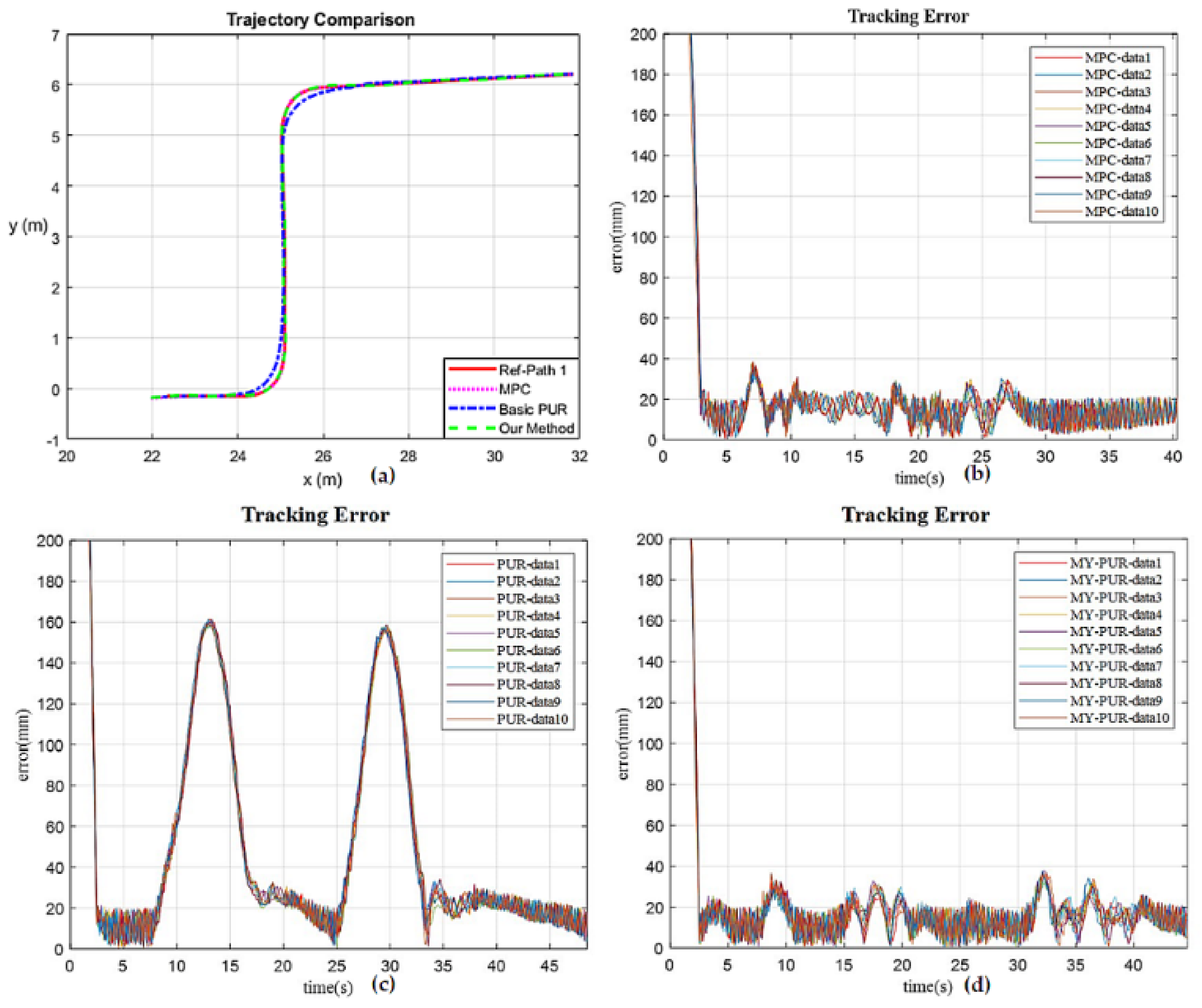
5.1. Trajectory-Tracking Accuracy Experiment

This experiment will verify the trajectory-tracking accuracy of the proposed method in this paper. The experimental method sets two preset paths. The first is the Double-L-shaped path, as shown in Figure 12a, and the second is the S-shaped path, as shown in Figure 13a. The coordinates reached by the mobile robot during navigation and the trajectory errors of the preset paths are recorded. The experiment is repeated 10 times on each path from the same starting point. The Model Predictive Control (MPC) and the original Pure Pursuit (PP) are used to compare in this paper, as shown in

Table 2. Results of Trajectory-Tracking Accuracy Experiment. MPC stands for Model Predictive Control method, PP stands for Pure Pursuit method.

Trajectory-Tracking Algorithm	Maximum Error (mm)	Average Error (mm)	Standard Deviation of Error (mm)
Double-L-shaped path (14.9 m)
MPC	35.959	14.644	±0.131
PP	160.215	48.158	±0.289
Our improved PP	35.967	14.892	±0.223
S-shaped path (8.2 m)
MPC	34.282	19.329	±0.449
PP	202.026	91.625	±0.885
Our improved PP	44.609	15.742	±0.330

. Because the starting point is joystick migration, there is a slight artificial error at the starting point, and the error data are calculated after 5 s. The results verified that the maximum error of the improved Pure Pursuit is within 45 mm, with a 77% improvement rate compared to the original Pure Pursuit, while our method has a similar error rate as the MPC method.

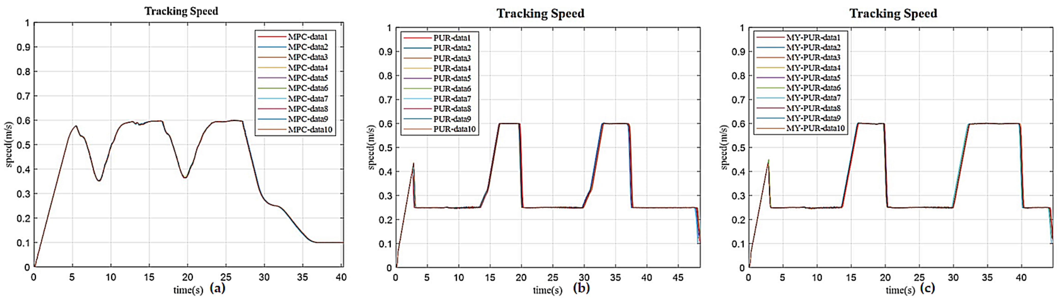
5.2. Trajectory-Tracking Speed Experiment

Besides accuracy, speed is also an essential factor. Thus, the verification experiment was conducted. According to Figure 14 and Figure 15, and

Table 3. Results of Trajectory-Tracking Speed Experiment. MPC stands for Model Predictive Control method, PP stands for Pure Pursuit method.

Trajectory-Tracking Algorithm	Average Speed (m/s)	Task Time (s)	Standard Deviation of Speed (s)
Double-L-shaped path (14.9 m)
MPC	0.396	40.31	±0.070
PP	0.322	48.42	±0.125
Our improved PP	0.358	44.63	±0.078
S-shaped path (8.2 m)
MPC	0.287	22.92	±0.060
PP	0.248	25.93	±0.118
Our improved PP	0.262	25.43	±0.064

, the average speed, task time and speed standard deviation of the improved PP are better than those of the original PP. The speed performance of the Double-L-shaped path increases by $11.2\%$ and the speed of the S-shaped path increases by $5.6\%$. The performance of the improved PP is similar MCP method. This experiment proves that the improved PP performs tasks more efficiently.

5.3. Verifying the Deep Learning-Based Localization Switching Method to Solve Corridor Effect

The location of the experiment is a corridor at the National Taiwan University of Science and Technology, as shown in Figure 16. The red line is the ground truth of the experiment. Marks are spaced every 5 m, and the total length is 88 m.

5.3.1. Evaluation of the Deep Learning-Based Corridor Recognition Method

Because we consider the corridor recognition problem as the binary classification problem, we collect two types of point-cloud data: the data of corridor area and the data of non-corridor data. Then we preprocess the collected 2D LiDAR images as mentioned in Section 4.2 and split the training/test dataset in a ratio of 9:1. Furthermore, due to small amount of 2D LiDAR data, we apply some data augmentation operations, such as flip and rotation, to enrich training data. As shown in

Table 4. Results of corridor recognition models.

Models	Accuracy (%)	Number of Parameters
SVM [25]	80%	-
InceptionV3-based model	100%	~22 million
LeNet-based model	100%	~1.1 million

, compared to the traditional Support Vector Machine (SVM) [24] classifier, the deep learning-based.

Models have better accuracy results in the test dataset. The LeNet-based model has only about 1.2 million parameters for the model size comparison, while its accuracy is similar to the bigger InceptionV3-based model. This guarantees that our proposed deep-learning-based model can be deployed on AGV and give a reliable and effective performance.

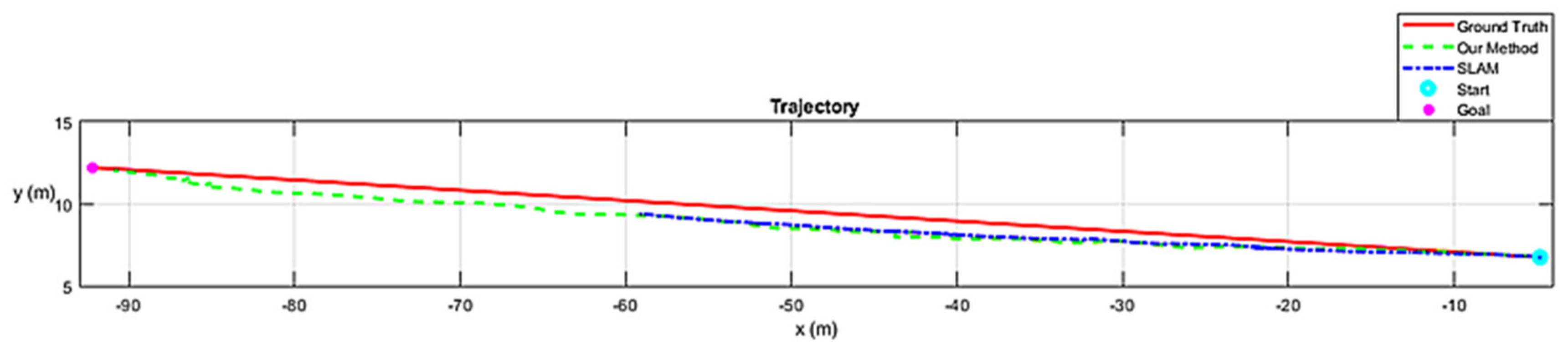
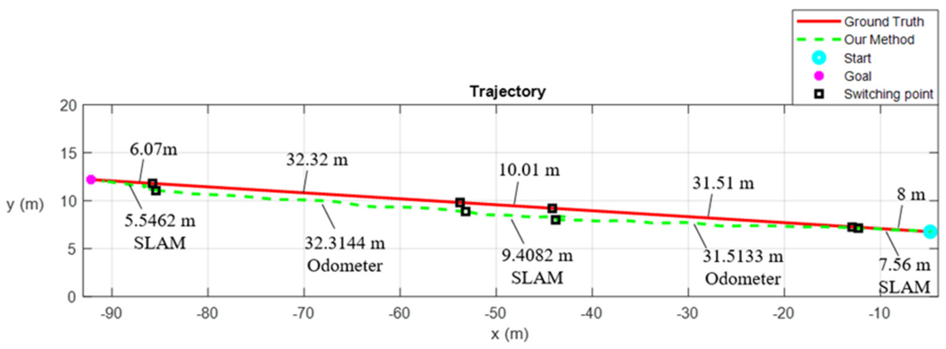
5.3.2. Verification of the Localization Switching Method in Practice

On the experimental corridor, we first manually move the mobile robot along the ground truth to record the trajectory of SLAM localization. Simultaneously, the deep learning-based classifier also is used to detect the long corridor regions. As the experimental results (shown in Figure 17 and Figure 18 and

Table 5. Results of corridor recognition models.

Experiment	Track Length (m)
Ground Truth	88
SLAM	54.4
Our Method	86.3

), it is impossible to complete the trajectory tracking and localization task if using SLAM only. Otherwise, by switching between SLAM and odometry localization system using our proposed method, the AGV can complete the trajectory tracking even in sparse LiDAR feature environment. Our experimental results proved the effectiveness of the deep learning-based localization switching method that involve improved Pure Pursuit robustness and feasibility.

6. Conclusions

To improve the trajectory-tracking accuracy of the original Pure Pursuit algorithm when following the turning path, we propose an improved Pure Pursuit algorithm that adds the functions of predicting the next turn and adjusting speed in the current turn. In structure-less environment AGV localization, this paper introduces a deep-learning-based corridor area classifier using 2D LiDAR data to select a suitable localization system to solve the corridor effect. The practical experimental results verified that the maximum error of the modified Pure Pursuit is within 45 mm, with a 77% improvement rate compared to the original Pure Pursuit. The improved Pure Pursuit algorithm also increased the speed by more than 5.6%. Moreover, the proposed localization switching method using deep learning helps to increase 36.25% of completion rate higher than that only using SLAM localization, prove the robust effectiveness of the proposed method in practice.

References

1. Chang, L.; Shan, L.; Li, J.; Dai, Y. The Path Planning of Mobile Robots Based on an Improved A* Algorithm. In Proceedings of the 2019 IEEE 16th International Conference on Networking, Sensing and Control (ICNSC), Banff, AB, Canada, 9–11 May 2019; pp. 257–262. [Google Scholar]
2. Zeng, Z.; Sun, W.; Wu, W.; Xue, M.; Qian, L. An Efficient Path Planning Algorithm for Mobile Robots. In Proceedings of the 2019 IEEE 15th International Conference on Control and Automation (ICCA), Edinburgh, UK, 16–19 July 2019; pp. 487–493. [Google Scholar]
3. Li, Y.; Huang, Z.; Xie, Y. Path planning of mobile robot based on improved genetic algorithm. In Proceedings of the 2020 3rd International Conference on Electron Device and Mechanical Engineering (ICEDME), Suzhou, China, 1–3 May 2020; pp. 691–695. [Google Scholar]
4. Zhang, L.; Zhang, Y.; Li, Y. Mobile Robot Path Planning Based on Improved Localized Particle Swarm Optimization. IEEE Sens. J. 2020, 21, 6962–6972. [Google Scholar] [CrossRef]
5. Wu, H.; Si, Z.; Li, Z. Trajectory Tracking Control for Four-Wheel Independent Drive Intelligent Vehicle Based on Model Predictive Control. IEEE Access 2020, 8, 73071–73081. [Google Scholar] [CrossRef]
6. Li, S.; Li, Z.; Yu, Z.; Zhang, B.; Zhang, N. Dynamic trajectory planning and tracking for autonomous vehicle with obstacle avoidance based on model predictive control. IEEE Access 2019, 7, 132074–132086. [Google Scholar] [CrossRef]
7. Yang, T.; Li, Z.; Yu, J. Trajectory Tracking Control of Surface Vehicles: A Prescribed Performance Fixed-Time Control Approach. IEEE Access 2020, 8, 209441–209451. [Google Scholar] [CrossRef]
8. Amer, N.H.; Hudha, K.; Zamzuri, H.; Aparow, V.R.; Abidin, A.F.Z.; Kadir, Z.A.; Murrad, M. Adaptive Trajectory Tracking Controller for an Armoured Vehicle: Hardware-in-the-loop Simulation. In Proceedings of the 2018 57th Annual Conference of the Society of Instrument and Control Engineers of Japan (SICE), Nara, Japan, 11–14 September 2018; pp. 462–467. [Google Scholar]
9. Yan, F.; Li, B.; Shi, W.; Wang, D. Hybrid visual servo trajectory tracking of wheeled mobile robots. IEEE Access 2018, 6, 24291–24298. [Google Scholar] [CrossRef]
10. Chen, Y.; Shan, Y.; Chen, L.; Huang, K.; Cao, D. Optimization of Pure Pursuit Controller based on PID Controller and Low-pass Filter. In Proceedings of the 2018 21st International Conference on Intelligent Transportation Systems (ITSC), Maui, HI, USA, 4–7 November 2018; pp. 3294–3299. [Google Scholar]
11. Wang, W.-J.; Hsu, T.-M.; Wu, T.-S. The improved pure pursuit algorithm for autonomous driving advanced system. In Proceedings of the 2017 IEEE 10th International Workshop on Computational Intelligence and Applications (IWCIA), Hiroshima, Japan, 11–12 November 2017; pp. 33–38. [Google Scholar]
12. Wang, R.; Li, Y.; Fan, J.; Wang, T.; Chen, X. A Novel Pure Pursuit Algorithm for Autonomous Vehicles Based on Salp Swarm Algorithm and Velocity Controller. IEEE Access 2020, 8, 166525–166540. [Google Scholar] [CrossRef]
13. Yousif, K.; Bab-Hadiashar, A.; Hoseinnezhad, R. An Overview to Visual Odometry and Visual SLAM: Applications to Mobile Robotics. Intell. Ind. Syst. 2015, 1, 289–311. [Google Scholar] [CrossRef]
14. Rozenberszki, D.; Majdik, A.L. LOL: Lidar-only Odometry and Localization in 3D point cloud maps. In Proceedings of the 2020 IEEE International Conference on Robotics and Automation (ICRA), Paris, France, 31 May–31 August 2020; pp. 4379–4385. [Google Scholar]
15. Zhao, S.; Zhang, H.; Wang, P.; Nogueira, L.; Scherer, S. Super Odometry: IMU-centric LiDAR-Visual-Inertial Estimator for Challenging Environments. arXiv 2021, arXiv:2104.14938. [Google Scholar]
16. Cho, H.; Kim, E.K.; Kim, S. Indoor SLAM application using geometric and ICP matching methods based on line features. Robot. Auton. Syst. 2018, 100, 206–224. [Google Scholar] [CrossRef]
17. Millane, A.; Oleynikova, H.; Nieto, J.; Siegwart, R.; Cadena, C. Free-Space Features: Global Localization in 2D Laser SLAM Using Distance Function Maps. In Proceedings of the 2019 IEEE/RSJ International Conference on Intelligent Robots and Systems (IROS), Macau, China, 3–8 November 2019; pp. 1271–1277. [Google Scholar]
18. Szegedy, C.; Vanhoucke, V.; Ioffe, S.; Shlens, J.; Wojna, Z. Rethinking the Inception Architecture for Computer Vision. In Proceedings of the 2016 IEEE Conference on Computer Vision and Pattern Recognition (CVPR), Las Vegas, NV, USA, 27–30 June 2016; pp. 2818–2826. [Google Scholar]
19. Redmon, J.; Farhadi, A. YOLOv3: An Incremental Improvement. arXiv 2018, arXiv:1804.02767. [Google Scholar]
20. Chen, J.; Ye, P.; Sun, Z. Pedestrian Detection and Tracking Based on 2D Lidar. In Proceedings of the 2019 6th International Conference on Systems and Informatics (ICSAI), Shanghai, China, 2–4 November 2019; pp. 421–426. [Google Scholar]
21. Luo, R.C.; Hsiao, T.J. Kidnapping and Re-Localizing Solutions for Autonomous Service Robotics. In Proceedings of the IECON 2018—44th Annual Conference of the IEEE Industrial Electronics Society, Washington, DC, USA, 21–23 October 2018; pp. 2552–2557. [Google Scholar]
22. Luo, R.C.; Yeh, K.C.; Huang, K.H. Resume navigation and re-localization of an autonomous mobile robot after being kidnapped. In Proceedings of the 2013 IEEE International Symposium on Robotic and Sensors Environments (ROSE), Washington, DC, USA, 21–23 October 2013; pp. 7–12. [Google Scholar]
23. Hess, W.; Kohler, D.; Rapp, H.; Andor, D. Real-time loop closure in 2D LIDAR SLAM. In Proceedings of the 2016 IEEE International Conference on Robotics and Automation (ICRA), Stockholm, Sweden, 16–21 May 2016; pp. 1271–1278. [Google Scholar]
24. LeCun, Y.; Bottou, L.; Bengio, Y.; Haffner, P. Gradient-based learning applied to document recognition. Proc. IEEE 1998, 86, 2278–2324. [Google Scholar] [CrossRef] [Green Version]
25. Cortes, C.; Vapnik, V. Support-vector networks. Mach. Learn. 1995, 20, 273–297. [Google Scholar] [CrossRef]
Figure 1. The schematic diagram of mobile robot hardware platform.
Applsci 11 05963 g001
Figure 2. The schematic diagram of the differential-wheel model.
Applsci 11 05963 g002
Figure 3. The definition of the target point g (blue circle) in Pure Pursuit algorithm.
Applsci 11 05963 g003
Figure 4. The control structure block diagram of PD controller.
Applsci 11 05963 g004
Figure 5. The impact of forward-looking (foresight) distance on generating the tracking error in the Pure Pursuit algorithm. A longer forward-looking distance represents smoother path tracking, and a shorter forward-looking distance give accurate tracking, but the PD controller is more challenging to adjust.
Applsci 11 05963 g005
Figure 6. The impact forward-looking distance in trajectory-tracking.
Applsci 11 05963 g006
Figure 7. The turning decision strategy of the proposed improved forward-looking distance tracking. (a) Predict Turn: Predicting a front turn or not. (b) Turn Now: Making the turn action. (c) Rugged Route: Making a turn in the case of rugged route.
Applsci 11 05963 g007
Figure 8. The curve prediction in the ideal case and the actual case.
Applsci 11 05963 g008
Figure 9. The environment map constructed by 2D LiDAR; black indicates obstacles (e.g., walls); white indicates no obstacles and gray represents unknown areas.
Applsci 11 05963 g009
Figure 10. (a) Mobile robot receives point-cloud range. (b) Point-cloud is drawn on picture.
Applsci 11 05963 g010
Figure 11. The preprocessing for 2D LiDAR images.
Applsci 11 05963 g011
Figure 12. The path error comparison between MPC (purple), original PP (blue) and proposed improved PP (green) methods in Double-L-shaped path (red): (a) Trajectory comparison chart. (b) MPC trajectory error path. (c) Original PP trajectory error graph. (d) Improved PP trajectory error graph.
Applsci 11 05963 g012
Figure 13. The path error comparison between MPC (purple), original PP (blue) and proposed improved PP (green) methods in S-shaped path (red): (a) Trajectory comparison chart. (b) MPC trajectory error path. (c) Original PP trajectory error graph. (d) Improved PP trajectory error graph.
Applsci 11 05963 g013
Figure 14. The speed comparison between MPC, original PP and proposed improved PP methods in Double-L-shaped path: (a) MPC speed curve. (b) Original PP speed curve. (c) Improved PP speed curve.
Applsci 11 05963 g014
Figure 15. The speed comparison between MPC, original PP and proposed improved PP methods in S-shaped path: (a) MPC speed curve. (b) Original PP speed curve. (c) Improved PP speed curve.
Applsci 11 05963 g015
Figure 16. The practical corridor environment for experiments.
Applsci 11 05963 g016
Figure 17. The tracked trajectory comparison. The red line is the ground truth, The blue line is the SLAM method, and the green line is our method’s trajectory method.
Applsci 11 05963 g017
Figure 18. The complete trajectory tracking of our proposed method in practice.
Applsci 11 05963 g018