Modeling a New AQM Model for Internet Chaotic Behavior Using Petri Nets

Abstract

Formal modeling is considered one of the fundamental phases in the design of network algorithms, including Active Queue Management (AQM) schemes. This article focuses on modeling with Petri nets (PNs) a new scheme of AQM. This innovative AQM is based on a discrete dynamical model of random early detection (RED) for controlling bifurcations and chaos in Internet congestion control. It incorporates new parameters $\left(\alpha ,\beta \right)$ that make possible better stability control over oscillations of an average queue length (AQL) at the router. The PN is validated through the matrix equation approach, reachability tree, and invariant analysis. The correctness is validated through the key properties of reachability, boundedness, reversibility, deadlock, and liveness.

1. Introduction

The Internet is a network that is designed to handle the load of streams of diverse traffic. Since its invention more than five decades ago [1,2], the Internet has become a key instrument for billions to stay in contact with everyone, and its expansion has been uninterrupted. At the time this writing, with much of the world staying at home due to the worldwide pandemic situation, the Internet is experiencing an unprecedented surge in usage. In consequence, an evident increase in Internet traffic has been caused by manifold online activities, such as remote working, distance learning, and video calls, among others. In Ref. [3], the impact on the Internet performance (latency, packet loss, etc.) of the COVID-19 lockdown is evaluated. Due to this extraordinary situation for data networks, the topic of congestion control has arisen and needs active queue management (AQM) algorithms in routers supporting Internet traffic. AQM algorithms should be able to actively control the average queue length (AQL) and thus to be able to prevent congestion as much as possible. A large increase in traffic and poor congestion control can cause network performance to partially or fully degrade and, consequently, impact applications. In addition, the design process of AQM schemes should make use of formal description techniques in the various steps of implementation. This article is an extended version of the outcomes appearing in [4]; it focuses on modeling with Petri nets (PNs) a new discrete dynamical model of AQM for congestion control, due to the chaotic behavior of Internet traffic. The PN formalism is a powerful method for modeling, and the precise nature of the graphical representation facilitates the understanding of the behavior of our AQM. For validation, we used PN mathematical methods that satisfy key properties, such as reachability, boundedness, reversibility, deadlock, and liveness.

The remainder of this article is organized as follows. Section 2 presents the related work and motivation—chaotic behavior of Internet traffic, congestion control, and formal description techniques. Section 3 introduces our dynamical model of AQM. Section 4 presents our solution based on Petri nets. Section 5 discusses the validation and correctness. Section 6 shows the numerical simulations and performance study based on the outcomes appearing in [4]. Finally, Section 7 presents the conclusions and ongoing work.

2. Related Work and Motivation

Chaos means deterministic behavior that is sensitive to its initial condition. The branch of mathematics known as dynamical systems, discrete and continuous, uses bifurcation theory [5] to study chaos in multiple fields, including engineering (see [6,7,8,9,10]). A bifurcation occurs when a small, smooth change made to the parameter values of a system causes a sudden qualitative or topological change in its general behavior. Generally, a bifurcation diagram shows the possible long-term values (equilibria/fixed points or periodic orbits) of a chaotic system as a function of a bifurcation parameter in the system. It is usual to represent stable solutions with a solid line and unstable solutions with a dotted line.

The majority of Internet traffic is generated and controlled by Transmission Control Protocol (TCP), which has chaotic properties: nonlinearity, determinism, order in disorder, sensitivity to initial conditions, and unpredictability. Several decades ago, these major features in Transmission Control Protocol/Internet Protocol (TCP/IP) networks were demonstrated through the phenomenon called the fractal nature of Internet traffic [11]. Thus, it was revealed how extreme sensitivity to initial conditions (also known as the butterfly effect) and odd periodicity are inherent properties in TCP/IP networks that support fundamental applications such as web and electronic mail transmission, respectively, among others. Dynamical systems study internet behavior through bifurcation theory, modeling and reproducing the complexity of chaotic behavior of the TCP-like model for congestion control (see [11,12,13,14,15,16,17]).

In addition, queue management in routers plays an important role in taking care of congestion from network traffic. Thus, one of the main functions of AQM is to detect emerging congestion early, before the queues in the routers overflow and the packets are dropped [18]. Numerous studies on AQM congestion control schemes have been proposed (see [19,20,21,22]), and among different taxonomies, they can be classified into the queue-based category. These schemes do not directly control the arrival rate at the queue, the congestion is observed by the average or instantaneous queue length, and the aim is to stabilize the queue length. How to stabilize the queue length around an expected target regardless of nonlinear traffic loads requires fine-tuning of when and how to govern buffering and queue management. Moreover, queue-based AQM schemes have been studied from the perspective of chaos theory that also solve congestion control problems by using bifurcation analysis (see [23,24,25,26]).

Regarding the design of new communication protocols, including AQM schemes, the literature offers various formal description techniques (FDT) [27] that cover all relevant phases from specification to validation. As evidence, the majority of worldwide institutes of standardization in telecommunications, such as the International Organization for Standardization (ISO), the International Telecommunication Union (ITU), the European Telecommunications Standards Institute (ETSI), the Institute of Electrical and Electronics Engineers (IEEE), the Internet Research Task Force (IETF), and others, recognize the wide spectrum of FDT [27]: Specification and Description Language (SDL), Simple ProMeLa Interpreter (Spin), Language Of Temporal Ordering Specifications (LOTOS), Estelle, and Petri nets, among others.

Many of these FDT offer a complementary approach based on mathematical properties, which can be automatically applied to design and validate the correctness of an algorithm. In this article, we will use Petri nets (PNs) as FDT that are applied to the field of telecommunications engineering (see [28,29,30,31]. Due to space constraints in this article, the reader is directed to [28] for further explanation concerning the mathematical properties of the PNs that are used in Section 4. The next section introduces our dynamical model of queue-based AQM.

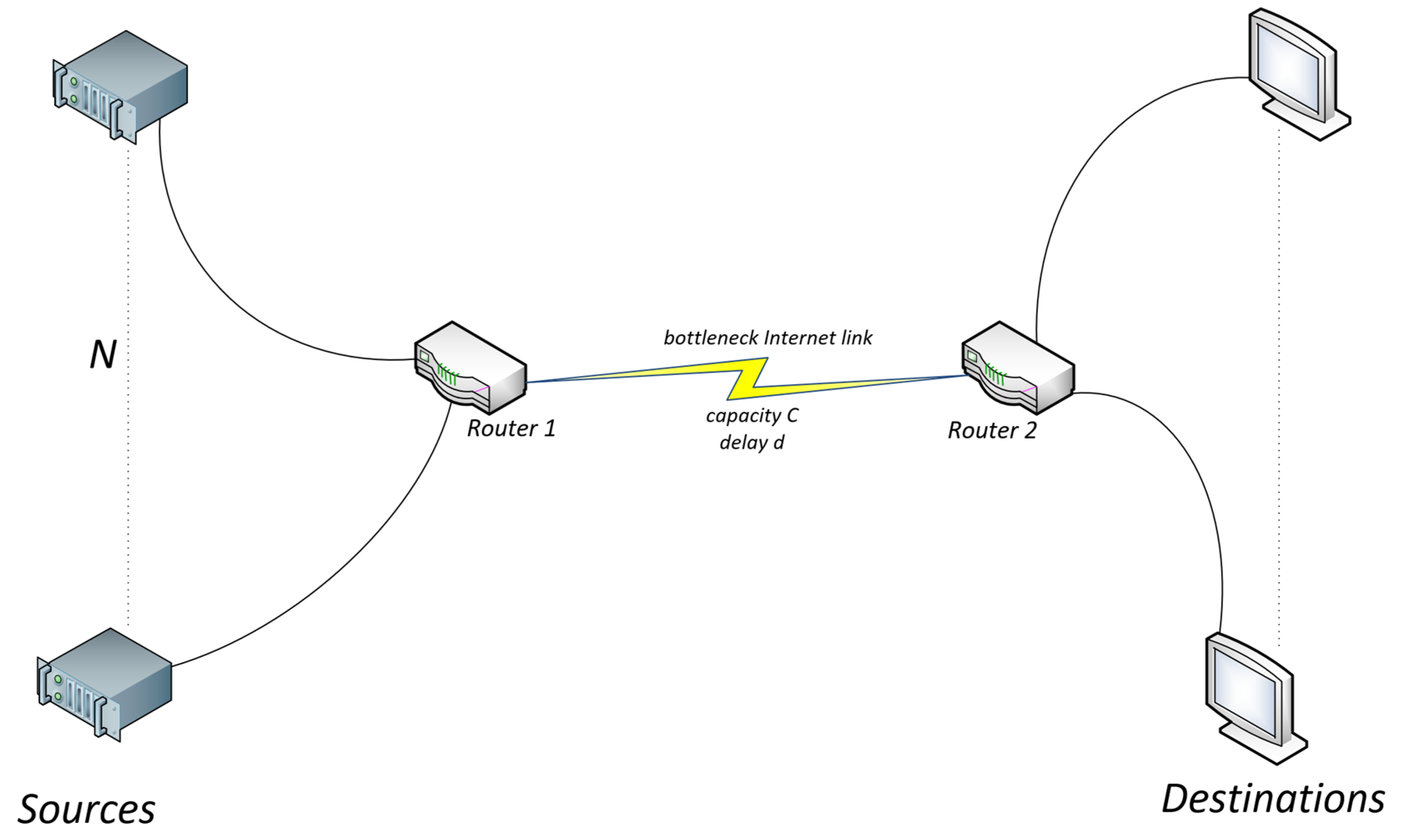
3. Dynamical Model for Congestion Control

Definition of Our Dynamical Model

Random early detection (RED) [32] is considered the pioneer queue-based AQM, and it is one of the most extensively investigated techniques for congestion avoidance. However, RED and its variants (see [33,34,35,36,37,38,39]), among others, suffer from parametrization problems, and community research is still ongoing to study new modifications, some of them using chaos theory (see [23,24,25,26]). The presented dynamical model of AQM is based on a generalization of the RED algorithm that improves performance. It uses the moving average of the queue length (AQL) to detect congestion and makes possible better stability control over oscillations of the AQL. When the AQL is below a minimum threshold, the packets are put into the buffer at the router. When the AQL exceeds the maximum threshold, the packets are dropped. When the AQL is between the minimum and the maximum threshold, the packets are randomly dropped according to some control parameters of our AQM. Concretely, the linear dropped packet probability distribution p of typical RED is replaced by the beta distribution (Equation (1)), providing two additional parameters $\left(\alpha ,\beta \right)$ with the aim of increasing the controllability of RED dynamics. Namely:

$$p\left(x;\alpha ,\beta \right)=\{\begin{array}{c}0 x<q_{min},\\ p_{max}{I}_z\left(\alpha ,\beta \right) q_{min}\le x\le q_{max}, \\ 1 x>q_{max},\end{array}$$

(1)

$$I_z\left(\alpha ,\beta \right)=\frac{B\left(z;\alpha ,\beta \right)}{B\left(1;\alpha ,\beta \right)},$$

(2)

$$B\left(z;\alpha ,\beta \right)={{\displaystyle \int }}_0^z{t}^{\alpha -1} {\left(1-t\right)}^{\beta -1}dt, z=\frac{x-q_{min}}{q_{max}-q_{min}}$$

(3)

where $B\left(z;\alpha ,\beta \right)$ is the incomplete beta function (Equation (3)) and $I_z\left(\alpha ,\beta \right)$ is the regularized incomplete beta function (Equation (2)). The value of x represents the AQL; $q_{min}$ and $q_{max}$ are the minimum and maximum thresholds of the queue size, respectively; and $p_{max}\in \left[0,1\right]$ is a selected drop probability. One of the advantages of our AQM model is that for properly chosen $\alpha$ and $\beta$ values, the stability ranges extend beyond their bifurcation values in the original formulation (i.e., $\alpha =\beta =1$), which recovers the original model of RED. In Ref. [40], we provide a further mathematical perspective of our dynamical model presented in this article. Next, the Algorithm 1 shows a high-level view of how our AQM works for each packet arrival.

Algorithm 1. Drop mechanism for each packet arrival.

4. Formal Description of Our Dynamical Model Using Petri Nets

In this section, we present a formal description of our dynamical model of AQM using PNs. The precise nature of the PN graphical representation facilitates the understanding of the behavior of our AQM scheme represented in Figure 1.

To begin with, we introduce the fundamentals of PNs that are used for the formal specification of our AQM. Once the specification is introduced, PN theory and its analysis techniques based on algebraic methods are applied for verification and correctness. Due to space constraints in this article, the reader is directed to [28] for further explanation concerning the mathematical properties of PNs applied to the design and validation process.

A PN is a directed graph described by places (represented by circles) and transitions (represented by bars), which are connected to each other with arcs. Connections between nodes of the same type (i.e., place to place and transition to transition) are not allowed. The places can contain zero or more tokens (represented by dots) that fire the transitions. The dynamic structure of a PN is defined by the movements of tokens from one place to another and is referred to as marking, i.e., it represents the PN status according to the fired transitions. Our dynamical model of AQM is a PN represented by (P, T, F, W, G, M₀), where:

P = {P₁,…,P_n} is a finite set of n places. The places hold the token (or tokens) and show the PN marking during its evolution.

T = {T₁,…,T_m} is a finite set of m transitions. They are the active events of the PN, which are used to change the position of the token (or tokens) during the evolution of the PN. In addition, the transitions can have guards that can restrict their firing, and they must be evaluated as true for the transition to be fireable.

In addition, T and P are disjoint sets: P ∩ T = $\varnothing$, P ∪ T ≠ $\varnothing$.

F⊆(PxT)∪ (TxP). F is a set of arcs (flow relation), where (PxT) is a set I of input arcs, which connect places to transitions. A place p is called an input place of a transition t if there exists an input arc from p to t. Then, (TxP) is a set O of output arcs, which connect transitions to places. A place p is called an output place of a transition t if there exists an output arc from t to p. A transition (an event) has a certain number of input and output places representing the pre- and post-conditions of the event, respectively.

W: F → {1,2,3,…} is a weight function. The arcs are labeled with their weights (positive integers). Labels for unity weight are usually omitted. Consequently, a PN is said to be ordinary if all of its arc weights are 1s.

G = {G₁,…,G_m} are the guards. They are Boolean expressions constructed by using the variables to enable and fire the associated transition under certain conditions.

Mo = {M₁,…,M_n} is the initial marking. M is a marking state that assigns to each place a non-negative integer. If a marking assigns to the place p a non-negative integer k, we say that p is marked with k tokens. Graphically, we place k tokens in place p. A marking is denoted by a vector M of n components, where n is the total number of places. The p-th component of M, denoted by M(p), is the number of tokens in place p. M_o represents where the tokens are positioned initially.

Additionally, a PN follows some rules that our AQM model monitors as well. A transition t is said to be enabled if each input place p of t is marked with at least w(p, t) tokens, where w(p, t) is the weight of the arc from p to t. A firing of an enabled transition t removes w(p, t) tokens from each input place p of t and adds w(t, p) tokens to each output place p of t, where w(t, p) is the weight of the arc from t to p. Furthermore, an enabled transition t may or may not fire depending on whether the guards take place.

If there is a guard g in a transition t, the associated rules must be evaluated. For the above rules of transition enabling, there is a concept related to the capacity of a place p. Initially, it is assumed that each place p can accommodate an unlimited number of tokens. In addition, it is natural to consider an upper limit to the number of tokens that each place can hold. Each place p has an associated capacity K(p), the maximum number of tokens that p can hold. For a transition t to be enabled, there is an additional condition that the number of tokens in each output place p of t cannot exceed its capacity K(p) after firing t.

Once the structure and rules are presented, the PN depicted in Figure 1 represents our AQM model at initial marking M₀ = (1,0,0,0,0,0,0,0,0,1). There are 10 places (n = 10, P1,…, P10) and 12 transitions (m = 12, T1,…,T12).

Table 1. Places, transitions, and guards of AQM.

Place	Description
P1	A new packet comes from the Internet (network) to the router, which is ready.
P2	The packet is received.
P3	The AQM gets the average queue length (AQL) at the router.
P4	The packet is accepted because the AQL is below the min. threshold.
P5	The AQM gets the probability pmax Iz (α, β).
P6	The packet is rejected because the AQL is over the max. threshold.
P7	The packet is accepted (not discard the result of pmax Iz (α, β)).
P8	The packet is rejected (discard the result of pmax Iz (α, β)).
P9	The packet is put into the buffer queue to be transmitted to the destination.
P10	The AQM ready for receiving the next packet.
Transition	Description
T1	Input a new packet; the router is ready.
T2	Start the transmission of the packet once received.
T3	The AQL is below the min. threshold. Check guard G1.
T4	The AQL is between thresholds. Check guard G2.
T5	The AQL is over the max. threshold. Check guard G3.
T6	Fill the buffer with the received packet.
T7	Drop the packet; the AQL is over the max. threshold.
T8	Do not discard the packet. Check guard G4.
T9	Discard the packet. Check guard G5.
T10	Input the packet into the buffer.
T11	Reject the packet.
T12	Leave the buffer. The packet is transmitted.
Guard	Description
G1	$\left(q_{min}<AQL\right)=True$. Guard associated to transition T3
G2	$\left(q_{min}\le AQL\le q_{max}\right)=True$. Guard associated to transition T4
G3	$\left(AQL>q_{max}\right)=True$. Guard associated to transition T5
G4	Not Discard = True. Guard associated to transition T8
G5	Discard = True. Guard associated to transition T9

shows further details of our PN.

Each place shows where the token is located, and the transitions are actions of our AQM model. The guards are on transitions T3, T4, T5, T8, and T9. Regarding the capacity, the places have capacity K = 1 to show how our AQM runs actions on the packet and router. The PN starts on T1 enabled, i.e., there is an incoming packet, the router is ready (P1), and AQM is ready (P10). Once T1 and T2 are fired, our model gets the AQL.

As said before, transitions T3, T4, T5, T8, and T9 have guards that restrict their firing. The PN fires T3 or T5 (fill buffer or drop packet) if the AQL is below $q_{min}$ or over $q_{max}$, respectively. If the AQL evaluates $q_{min}\le AQL\le q_{max}$ as true, T4 starts and P5 gets the probability to detect where the stabilization is at the average router queue length. The PN fires T8 or T9, not to discard or discard the packet according to the value from probability $p_{max}{I}_z\left(\alpha ,\beta \right)$. T10 and T11 mean input buffer or reject packet—that is, whether the packet is filled into the buffer or discarded, respectively. T12 is fired when the packet leaves the buffer, and P10 restarts the PN for more incoming packets.

5. Validation

We used well-known methods in the literature [28] for the validation of the PN. We applies the matrix equation approach, reachability tree method, and invariant analysis.

5.1. Matrix Equation

In this approach, the validation is described by algebraic equations. First, we present the matrix equations that govern the dynamic behavior of our AQM (Figure 1). For a PN with n places and m transitions, the incidence matrix $C=(C_{ij})$, is a matrix $\left(n\times m\right)$ represented in Equation (4) and defined by $C^{ij}=C_{ij}^{+}-C_{ij}^{-}$, where the post-conditions matrix $C_{ij}^{+}=w\left(i,j\right)$ is the weight of the arc from transition j to its output place i, and the pre-conditions matrix $C_{ij}^{-}=w\left(j,i\right)$ is the weight of the arc to transition j from its input place i. The PN of our AQM is ordinary, i.e., all of its arc weights are 1s, and the interpretation is as follows:

$$\begin{array}{c}{C}_{ij}^{+}=\{\begin{array}{c}1, \mathrm{there} \mathrm{is} \mathrm{arc} \mathrm{from} t_j \mathrm{to} p_i\\ 0, \mathrm{there} \mathrm{is} \mathrm{arc} \mathrm{from} t_j \mathrm{to} p_i\end{array}\\ C_{ij}^{-}=\{\begin{array}{c}1, \mathrm{there} \mathrm{is} \mathrm{arc} \mathrm{from} p_i \mathrm{to} t_j\\ 0, \mathrm{there} \mathrm{is} \mathrm{arc} \mathrm{from} p_i \mathrm{to} t_j\end{array}\\ C=C^{\mathrm{+}}-C^{-} =(\begin{array}{cccccccccccc}0& 1& 0& 0& 0& 0& 0& 0& 0& 0& 0& 0\\ 1& 0& 0& 0& 0& 0& 0& 0& 0& 0& 0& 0\\ 0& 1& 0& 0& 0& 0& 0& 0& 0& 0& 0& 0\\ 0& 0& 1& 0& 0& 0& 0& 0& 0& 0& 0& 0\\ 0& 0& 0& 1& 0& 0& 0& 0& 0& 0& 0& 0\\ 0& 0& 0& 0& 1& 0& 0& 0& 0& 0& 0& 0\\ 0& 0& 0& 0& 0& 0& 0& 1& 0& 0& 0& 0\\ 0& 0& 0& 0& 0& 0& 0& 0& 1& 0& 0& 0\\ 0& 0& 0& 0& 0& 1& 0& 0& 0& 1& 0& 0\\ 0& 0& 0& 0& 0& 0& 1& 0& 0& 0& 1& 1\end{array})\\ \hspace{1em}\hspace{1em}\hspace{1em}\hspace{1em}\hspace{1em}\hspace{1em}\hspace{1em}\hspace{1em}\hspace{1em}-\left(\begin{array}{cccccccccccc}1& 0& 0& 0& 0& 0& 0& 0& 0& 0& 0& 0\\ 0& 1& 0& 0& 0& 0& 0& 0& 0& 0& 0& 0\\ 0& 0& 1& 1& 1& 0& 0& 0& 0& 0& 0& 0\\ 0& 0& 0& 0& 0& 1& 0& 0& 0& 0& 0& 0\\ 0& 0& 0& 0& 0& 0& 0& 1& 1& 0& 0& 0\\ 0& 0& 0& 0& 0& 0& 1& 0& 0& 0& 0& 0\\ 0& 0& 0& 0& 0& 0& 0& 0& 0& 1& 0& 0\\ 0& 0& 0& 0& 0& 0& 0& 0& 0& 0& 1& 0\\ 0& 0& 0& 0& 0& 0& 0& 0& 0& 0& 0& 1\\ 1& 0& 0& 0& 0& 0& 0& 0& 0& 0& 0& 0\end{array}\right) =\\ \left(\begin{array}{cccccccccccc}\mathrm{-1}& 1& 0& 0& 0& 0& 0& 0& 0& 0& 0& 0\\ 1& \mathrm{-1}& 0& 0& 0& 0& 0& 0& 0& 0& 0& 0\\ 0& 1& \mathrm{-1}& \mathrm{-1}& \mathrm{-1}& 0& 0& 0& 0& 0& 0& 0\\ 0& 0& 1& 0& 0& \mathrm{-1}& 0& 0& 0& 0& 0& 0\\ 0& 0& 0& 1& 0& 0& 0& \mathrm{-1}& \mathrm{-1}& 0& 0& 0\\ 0& 0& 0& 0& 1& 0& \mathrm{-1}& 0& 0& 0& 0& 0\\ 0& 0& 0& 0& 0& 0& 0& 1& 0& \mathrm{-1}& 0& 0\\ 0& 0& 0& 0& 0& 0& 0& 0& 1& 0& \mathrm{-1}& 0\\ 0& 0& 0& 0& 0& 1& 0& 0& 0& 1& 0& \mathrm{-1}\\ \mathrm{-1}& 0& 0& 0& 0& 0& 1& 0& 0& 0& 1& 1\end{array}\right)\end{array}$$

(4)

Second, the matrix equation approach calculates the PN evolution as a result of firing a transition T from M₀ to state $M$. For the case of one fired transition, this is done with the equation of state:

$$M=M_0+C·t_j,$$

(5)

where M₀ is the initial marking and C is the incidence matrix calculated in Equation (4). The vector $t_j$ is called the trigger vector, which contains all transitions as a column. The j-th component of $t_j$ is 1, which means that the transition ${\mathrm{T}}_j$ is fired, and the others are 0. In Equation (6), we show the evolution of our PN to the next marking when the transition T1 is fired, i.e., a new packet arrives from the network to the router in ready mode.

$$M=M_0+C·t_1 =\left(\begin{array}{c}1\\ 0\\ 0\\ 0\\ 0\\ 0\\ 0\\ 0\\ 0\\ 1\end{array}\right)+\left(\begin{array}{cccccccccccc}\mathrm{-1}& 1& 0& 0& 0& 0& 0& 0& 0& 0& 0& 0\\ 1& \mathrm{-1}& 0& 0& 0& 0& 0& 0& 0& 0& 0& 0\\ 0& 1& \mathrm{-1}& \mathrm{-1}& \mathrm{-1}& 0& 0& 0& 0& 0& 0& 0\\ 0& 0& 1& 0& 0& \mathrm{-1}& 0& 0& 0& 0& 0& 0\\ 0& 0& 0& 1& 0& 0& 0& \mathrm{-1}& \mathrm{-1}& 0& 0& 0\\ 0& 0& 0& 0& 1& 0& \mathrm{-1}& 0& 0& 0& 0& 0\\ 0& 0& 0& 0& 0& 0& 0& 1& 0& \mathrm{-1}& 0& 0\\ 0& 0& 0& 0& 0& 0& 0& 0& 1& 0& \mathrm{-1}& 0\\ 0& 0& 0& 0& 0& 1& 0& 0& 0& 1& 0& \mathrm{-1}\\ \mathrm{-1}& 0& 0& 0& 0& 0& 1& 0& 0& 0& 1& 1\end{array}\right)·\left(\begin{array}{c}1\\ 0\\ 0\\ 0\\ 0\\ 0\\ 0\\ 0\\ 0\\ 0\\ 0\\ 0\end{array}\right) =\left(\begin{array}{c}0\\ 1\\ 0\\ 0\\ 0\\ 0\\ 0\\ 0\\ 0\\ 0\end{array}\right)$$

(6)

In addition, the matrix equation approach can calculate the PN evolution with a sequence of fired transitions. Thus, a marking M is said to be reachable from M₀ if there exists a sequence of firings σ that transforms M₀ into M. This is done with the equation of state:

$$M=M_0+C·\sigma .$$

(7)

The vector $\sigma =t_{j1}+t_{j2}+\dots +t_{jk}$ is called the firing vector of the sequence of fired transitions $t_{j1}{t}_{j2}\dots t_{jk},$ where $j_i\in \left\{1,2,\dots ,m\right\}$. We show the evolution of our PN from M₀ to the marking equivalent to the dropped packet because the AQL is over the maximum threshold, i.e., the sequence of firings T1, T2, and T5 and the firing vector σ (1,1,0,0,1,0,0,0,0,0,0,0).

$$M=M_0+C·\sigma =\left(\begin{array}{c}1\\ 0\\ 0\\ 0\\ 0\\ 0\\ 0\\ 0\\ 0\\ 1\end{array}\right)+\left(\begin{array}{cccccccccccc}\mathrm{-1}& 1& 0& 0& 0& 0& 0& 0& 0& 0& 0& 0\\ 1& \mathrm{-1}& 0& 0& 0& 0& 0& 0& 0& 0& 0& 0\\ 0& 1& \mathrm{-1}& \mathrm{-1}& \mathrm{-1}& 0& 0& 0& 0& 0& 0& 0\\ 0& 0& 1& 0& 0& \mathrm{-1}& 0& 0& 0& 0& 0& 0\\ 0& 0& 0& 1& 0& 0& 0& \mathrm{-1}& \mathrm{-1}& 0& 0& 0\\ 0& 0& 0& 0& 1& 0& \mathrm{-1}& 0& 0& 0& 0& 0\\ 0& 0& 0& 0& 0& 0& 0& 1& 0& \mathrm{-1}& 0& 0\\ 0& 0& 0& 0& 0& 0& 0& 0& 1& 0& \mathrm{-1}& 0\\ 0& 0& 0& 0& 0& 1& 0& 0& 0& 1& 0& \mathrm{-1}\\ \mathrm{-1}& 0& 0& 0& 0& 0& 1& 0& 0& 0& 1& 1\end{array}\right)·\left(\begin{array}{c}1\\ 1\\ 0\\ 0\\ 1\\ 0\\ 0\\ 0\\ 0\\ 0\\ 0\\ 0\end{array}\right) =\left(\begin{array}{c}1\\ 0\\ 0\\ 0\\ 0\\ 1\\ 0\\ 0\\ 0\\ 0\end{array}\right)$$

(8)

Occasionally, the matrix equations can show that a marking M is unreachable from M₀. The previous implication is that if Equation (7) has no natural solution, then M is unreachable from M₀ for the firing vector $\sigma$. As evidence, we can see in our AQM that some states (places in the PN) are unreachable from M₀, e.g., the probability $p_{max}{I}_z\left(\alpha ,\beta \right)$ cannot be calculated only with T4 if the sequence of transitions T1 and T2 is not fired previously. Next, the analysis based on the reachable tree will show graphically the reachable states with the associated sequence of fired transitions using the equation of state Equation (7).

5.2. Reachability Tree

In this approach, the validation proves how our AQM model runs the different states once an incoming packet is received at the router. Concretely, this approach validates the PN graphically as a labeled graph in which the nodes are the different reachable markings of the PN. The nodes are connected by arcs labeled by the transition name. The reachability tree starts from the root, which is labeled with the initial marking M₀. For every new state reachable from the root, there is an arc labeled with the transition that once fired goes to that new marking of the PN. With all nodes, we proceed in a similar way as the case of the root. Figure 2 shows the reachability tree that covers every reachable state (markings at the PN) of our AQM model.

5.3. Invariance Analysis

Next, we introduce the invariance analysis of our model. Invariants look for properties that remain constant with respect to certain patterns of executing the PN. Furthermore, invariants are used later to prove the properties of our AQM, such as reversibility and boundedness. We use the two most widely studied classes of invariants for the PN [28]. First, a natural solution of the equation $\mathrm{C}·x=0$ is called a transition invariant (T-invariant). It indicates a sequence of transitions (firing vector x with one entry for each transition), which leads back to the initial marking M₀.

Table 2. T-invariants in our AQM.

T-Invariant	Content	Description
1T-inv	(1,1,1,0,0,1,0,0,0,0,0,1)	Accept packet, AQL below min. threshold
2T-inv	(1,1,0,0,1,0,1,0,0,0,0,0)	Drop packet, AQL over max. threshold
3T-inv	(1,1,0,1,0,0,0,1,0,1,0,1)	Accept packet, AQM probability function
4T-inv	(1,1,0,1,0,0,0,0,1,0,1,0)	Reject packet, AQM probability function

shows the T-invariants for our AQM. They are the different firing vectors that return to the initial state for the next incoming packet at the router. Figure 3 shows each T-invariant, with the transition flow colored in purple.

Second, a natural solution of the equation $y · C=0$ is called a place invariant (P-invariant). A P-invariant is a vector with one entry for each place. It indicates that the number of tokens in all reachable places satisfies some linear invariant. Once a P-invariant called y is calculated, the following holds for every reachable state $M:y·M_0=y · M$. P-invariants are more difficult to detect than T-invariants. This is because the former are involved with the entire space state and all possible executions directions of the system (AQM in our case).

Table 3. P-invariants in our AQM.

P-Invariant	Content	Description
1P-inv	(1,1,0,0,0,0,0,0,0,0)	Router ready, received packet
2P-inv	(0,1,1,1,1,1,1,1,1,1)	AQM in process, received packet

shows the P-invariants of our AQM for any reachable place M represented at the reachability tree of Figure 2.

For any reachable place M, the vector y (1,1,0,0,0,0,0,0,0,0) of the 1P-inv is a natural solution of the equation $y · C=0$ and it holds the linear invariant $y_{\mathrm{p}1}· M_0+y_{\mathrm{p}2}· M_0=y_{\mathrm{p}1}· M+y_{\mathrm{p}2}· M=1$, where $y_{\mathrm{pj}}$ =(0,...,0,1,0,…,0) and 1 is located in the j position. That is, the token can be only in one of the places $y_{\mathrm{p}1}$ or $y_{\mathrm{p}2}$. This P-invariant (1P-inv) indicates a similarity with the mutual exclusion behavior in our AQM. Initially, P1 holds a token, and, once transition T1 is fired, the token moves to place P2. Next, transition T2 is fired, and P1 holds the token at the same time that our AQM continues processing the packet through place P3. Figure 4 shows how the token can be in places P1 or P2 but never in both in any reachable marking place, i.e., the router is ready for a new packet once the current one has passed to AQM.

Additionally, we studied the P-invariant 2P-inv. For any reachable place M, the vector y (0,1,1,1,1,1,1,1,1,1) of the 2P-inv is a natural solution of the equation $\mathrm{y} · \mathrm{C}=0$ and it holds the linear invariant $y_{p2}· M_0+y_{p3}· M_0+y_{p4}· M_0+y_{p5}· M_0+y_{p6}· M_0+y_{p7}· M_0+y_{p8}· M_0+y_{p9}· M_0+y_{p10}{M}_0= y_{p2}· M+y_{p3}· M+y_{p4}· M+y_{p5}· M+y_{p6}· M+y_{p7}· M+y_{p8}· M+y_{p9}· M+y_{p10}· M=1$ . Figure 4 shows how the token can be only in one of the places $y_{p2},y_{p3},y_{p4},y_{p5},y_{p6},y_{p7},y_{p8},y_{p9},$ or $y_{p10}$, i.e., the AQM is processing the packet.

5.4. Analysis of Properties

Once our scheme was validated with different methods, we proved the major properties.

5.4.1. Reachability

Reachability is a central property that is present in our AQM model. This proves that our AQM model can execute different states once an incoming packet is received from the network and reaches the router. The reachability tree (Figure 2) shows how every state of our AQM is reachable, some of them by different vectors of transitions.

5.4.2. Boundedness

Boundedness prevents information from getting lost, i.e., our AQM runs every incoming packet using our dynamical model. In a PN, a place p is said to be k-bounded if the number of tokens does not exceed a number $k\in \mathbb{N}$ for any marking reachable from M₀. In this article, we used $k=1$ to show how each packet is processed in our AQM. Boundedness has also been proved in the analysis of P-invariants (Table 3). We also studied boundedness with K = buffer length, i.e., changing the capacity of places in the PN represented in Figure 1.

5.4.3. Reversibility

Reversibility shows the life cycle of our AQM running each packet coming from the Internet (or network) to the router. A PN is said to be reversible if for each marking state M, the initial marking M₀ is reachable from M. The reachability tree showed how the different markings (nodes in Figure 2) return to the initial node to process the next packet. Our AQM is restarted through the node (1,0,0,0,0,0,0,0,0,1), the P1 router ready for the next packet, and the P10 AQM is ready for receiving the next packet. Reversibility is demonstrated also by the T-invariants (Table 2), which return the AQM model to the initial state M₀.

5.4.4. Deadlock

Deadlock is the state of a system, in our case the AQM model, in which no action can take place. A PN is said to be deadlock free if for any reachable marking state M, there is an enabled transition. That is, the PN is in deadlock if no transition is enabled at marking state M. Figure 2 shows how every reachable state (node in the reachability tree) fires a transition next. That is an important property of our AQM model, i.e., it is deadlock free.

5.4.5. Liveness

Liveness ensures that a system eventually enters into a state, i.e., the system is live. A PN is said to be alive if whatever marking state M is reached from M₀, it is possible to enable any transition at least once through some firing sequence. Figure 2 shows how every transition can be fired. This property ensures that our solution effectively performs its intended functions.

6. Numerical Simulations

Our AQM model, programmed with Python and Mathematica, followed the overall design presented before with PNs. Next, we present the performance of our dynamical model of AQM in comparison with the traditional RED algorithm. It was validated through numerical simulations and bifurcation analysis of the parameters $\alpha ,\beta$ on the AQL. This section is based on the outcomes of [4], and the reader is directed to [4] for further details.

6.1. Simulation Scenario

The simulation scenario (Figure 5) was a network where a dominant bottleneck link is shared by many connections. The scenario ran with a set of parameters, as given in [4].

In this scenario, we interpreted the shared link as an intercontinental Internet link with capacity C, and we assumed that the set of connections N uniformly have the same round-trip propagation delay d (without any queueing delay). Rather than interpreting this assumption as a requirement that the connections must have the same propagation delay, we considered d as the effective delay that represents the overall propagation delay of the connections, or this could describe a case where the bottleneck link has a large propagation delay that dominates the round-trip delays of the connections.

6.2. Performance Study

The aim of this section is to show numerically the advantages of introducing two new degrees of freedom in the probability function of the RED algorithm. It is well known that the combination of TCP end-to-end congestion control and RED active queue management can be modeled as a discrete-time dynamic system and that this system exhibits a variety of irregular behaviors, such as bifurcation and chaos. A great amount of research has been devoted to tune RED parameters to achieve good performance in different congestion scenarios.

For our study, we used the first-order nonlinear dynamic feedback model given in [24]. Considering this model, we performed a biparametric sweep of α and β ranging from the 0.4 to 1, and for each of these values, we studied the behavior of two important characteristics that provide information about the performance and stability of the system, namely, the first bifurcation point when we consider as a bifurcation parameter the number of connections (Figure 6a) and the average queue length when the system reaches stability (Figure 6b).

Numerical simulations showed that there are regions of the biparametric spectrum where the system behavior presents much more favorable scenarios. Therefore, the parameters can be adapted to improve the performance and stability of the network, depending on the characteristics of the congestion scenarios, such as the number of connections, the bandwidth, and the round-trip propagation delay. In Ref. [41], bifurcation diagrams for specific values in different scenarios are discussed.

7. Conclusions

The issue of congestion control is still open, and one of the most important goals for AQM schemes is how to manage the drop probability when congestion occurs. In this article, we used PNs as a formal method for the design of a new AQM model that contributes to detecting where stabilization occurs at the AQL. PN formalism is demonstrated to be a powerful method for the mathematical modeling of our AQM scheme. For the validation of our AQM scheme, the methods of PNs demonstrated to satisfy the key properties of reachability, boundedness, reversibility, deadlock, and liveness. To conclude this article, we give further details of ongoing work.

Ongoing Work

Once our AQM scheme is designed and validated mathematically, network simulation is highly recommended prior to real development. Our ongoing work is the implementation of our AQM model on the network simulator NS3 [42]. This section shows the primary details related to the accurate preparation of the traffic to be configured in the simulator. First, the limitations of network simulators [43] when the simulation scenarios should simulate the complex reality of the Internet are well known. Second, the question of Internet traffic characterization has taken a long research history [44,45,46,47], and for a long time, the Internet Engineering Task Force (IETF) [48] has recognized that it has been an important challenge for network researchers and operators. The literature says also that the identification and classification of network traffic are an important pre-requisite of network management and also gives importance to the packet size distribution of typical Internet applications [47]. Thus, we study the Internet traffic behavior by running real traffic traces, and we must find a methodology that can characterize this traffic in the simulator. At the time of writing this section, we made a study of the traffic created in our campus network (see Figure 7 and Figure 8). These graphs of statistics represent the number of TCP connections per second and the bandwidth used (megabits per second) in the link of our campus network to the Internet. The graphs were calculated with software for monitoring networks [49], and the traffic came from many TCP connections to different worldwide websites in the last week of March. We can see that the traffic is variable, since throughout the day, there are many peaks and valleys. We considered these values for different setups in the simulator, in conjunction with more parameters, such as buffer size, bandwidth delay, and packet length, among others. For the analysis of how fast our approach is, the software code of our AQM scheme is being implemented using, among others, metrics of optimal computational cost.

References

1. Kleinrock, L. An early history of the internet [History of Communications]. IEEE Commun. Mag. 2010, 48, 26–36. [Google Scholar] [CrossRef]
2. Leiner, B.; Cerf, V.; Clark, D.; Kahn, R.; Kleinrock, L.; Lynch, D.; Postel, J.; Roberts, L.; Wolff, S. The past and future history of the Internet. Commun. ACM 1997, 40, 102–108. [Google Scholar] [CrossRef]
3. Candela, M.; Luconi, V.; Vecchio, A. Impact of the COVID-19 pandemic on the Internet latency: A large-scale study. Comput. Netw. 2020, 182, 107495. [Google Scholar] [CrossRef]
4. Duran, G.; Valero, J.; Amigó, J.M.; Giménez, A.; Bonastre, O.M. Bifurcation analysis for the Internet congestion. In Proceedings of the IEEE INFOCOM, Paris, France, 29 April–2 May 2019; pp. 1073–1074. [Google Scholar]
5. Lorenz, E. Deterministic Non periodic Flow. J. Atmos. Sci. 1963, 20, 130–141. [Google Scholar] [CrossRef] [Green Version]
6. Moon, F.C. Chaotic and Fractal Dynamics: An Introduction for Applied Scientists and Engineers; Wiley: New York, NY, USA, 1992. [Google Scholar]
7. Banerjee, S.; Mitra, M.; Rondoni, L. Applications of Chaos and Nonlinear Dynamics in Engineering; Springer: Berlin/Heidelberg, Germany, 2011; Volume 1. [Google Scholar]
8. Karimov, A.; Tutueva, A.; Karimov, T.; Druzhina, O.; Butusov, D. Adaptive Generalized Synchronization between Circuit and Computer Implementations of the Rössler System. Appl. Sci. 2021, 11, 81. [Google Scholar] [CrossRef]
9. Karimov, T.; Nepomuceno, E.G.; Druzhina, O.; Karimov, A.; Butusov, D. Chaotic Oscillators as Inductive Sensors: Theory and Practice. Sensors 2019, 19, 4314. [Google Scholar] [CrossRef] [Green Version]
10. Tutueva, A.V.; Artur, I.K.; Moysis, L.; Volos, C.; Butusov, D.N. Construction of one-way hash functions with increased key space using adaptive chaotic maps. Chaos Solitons Fractals 2020, 141, 110344. [Google Scholar] [CrossRef]
11. Veres, A.; Boda, M. The chaotic nature of TCP congestion Control. In Proceedings of the IEEE INFOCOM, Tel Aviv, Israel, 26–30 March 2000; pp. 1715–1723. [Google Scholar]
12. Leland, W.E.; Taqqu, M.S.; Willinger, W.; Wilson, D.V. On the self-similar nature of Ethernet traffic. IEEE/ACM Trans. Netw. 1994, 2, 1–15. [Google Scholar] [CrossRef] [Green Version]
13. Cai, L.; Li, H.; Chen, B.; Wang, J. On the Chaotic Dynamics Analysis of Internet Traffic. In Proceedings of the International Workshop on Chaos-Fractals Theories and Applications, Shenyang, China, 6–8 November 2009; pp. 361–364. [Google Scholar]
14. Kaklauskas, L.; Sakalauskas, L. Application of Chaos Theory to Analysis of Computer Network Traffic. In Proceedings of the International Conference Applied Stochastic Models and Data Analysis, Vilnius, Lithuania, 30 June–3 July 2009; pp. 407–411. [Google Scholar]
15. Yan, G. Internet Congestion Control based on the Controlling Bifurcation and Chaos algorithm. In Proceedings of the IEEE International Conference on Mechatronics and Control, Jinzhou, China, 3–5 July 2014; pp. 1500–1503. [Google Scholar]
16. Rezaie, B.; Motlagh, M.; Khorsandi, S.; Analoui, M. Analysis and control of bifurcation and chaos in TCP-like Internet congestion control model. In Proceedings of the 15th International Conference on Advanced Computing and Communications, Guwahati, India, 18–21 December 2007; pp. 111–116. [Google Scholar]
17. Huang, Z.; Yang, Q.; Cao, J. The stochastic stability and bifurcation behavior of an Internet congestion control model. Math. Comput. Model. 2011, 54, 1954–1965. [Google Scholar] [CrossRef]
18. Jacobson, V. Congestion avoidance and control. ACM SIGCOMM Comput. Commun. Rev. 1998, 18, 314–329. [Google Scholar] [CrossRef]
19. Adams, R. Active queue management: A survey. IEEE Commun. Surv. Tutor. 2013, 5, 1425–1476. [Google Scholar] [CrossRef]
20. Nichols, K.; Jacobson, V. Controlling Queue Delay. ACM Queue 2012, 55, 42–50. [Google Scholar]
21. Alwahab, D.; Laki, S. A Simulation-Based Survey of Active Queue Management Algorithms. In Proceedings of the 6th International Conference on Communications and Broadband Networking, Singapore, 24–26 February 2018; pp. 71–77. [Google Scholar]
22. Chitra, K.; Padamavathi, G. Classification and Performance of AQM-Based Schemes for Congestion Avoidance. Int. J. Comput. Sci. Inf. Secur. 2010, 8, 331–340. [Google Scholar]
23. Zheng, Y.G.; Wang, Z.H. Stability and Hopf bifurcation of a class of TCP/AQM networks. Nonlinear Anal. Real World Appl. 2010, 11, 1552–1559. [Google Scholar] [CrossRef]
24. Ranjan, P.; Abed, E.H.; La, R.J. Nonlinear instabilities in TCP-RED. IEEE/ACM Trans. Netw. 2004, 12, 1079–1092. [Google Scholar] [CrossRef] [Green Version]
25. Ding, D.; Zhu, J.; Luo, X. Hopf bifurcation analysis in a fluid flow model of Internet congestion control algorithm. Nonlinear Anal. Real World Appl. 2009, 10, 824–839. [Google Scholar] [CrossRef]
26. Beneš, N.; Brim, L.; Pastva, S.; Šafránek, D. Digital Bifurcation Analysis of Internet Congestion Control Protocols. Int. J. Bifurc. Chaos 2020, 30, 2030038. [Google Scholar] [CrossRef]
27. Babich, F.; Deotto, L. Formal methods for specification and analysis of communication protocols. IEEE Commun. Surv. Tutor. 2002, 4, 2–20. [Google Scholar] [CrossRef] [Green Version]
28. Murata, T. Petri nets: Properties, analysis and applications. Proc. IEEE 1989, 77, 541–580. [Google Scholar] [CrossRef]
29. Tang, S.; Hu, X.; Zhao, L. Modeling and Security Analysis of IEEE 802.1AS Using Hierarchical Colored Petri Nets. In Proceedings of the IEEE GLOBECOM, Taipei, Taiwan, 8–10 December 2020; pp. 1–6. [Google Scholar]
30. Mahendran, V.; Gunasekaran, R.; Siva, C. Performance Modeling of Delay-Tolerant Network Routing via Queueing Petri Nets. IEEE Trans. Mob. Comput. 2014, 13, 1816–1828. [Google Scholar] [CrossRef]
31. Wang, C.; Tao, Y.; Zhou, Y. Protocol Verification by Simultaneous Reachability Graph. IEEE Commun. Lett. 2017, 21, 1727–1730. [Google Scholar] [CrossRef]
32. Floyd, S.; Jacobson, V. Random early detection gateways for congestion avoidance. IEEE Trans. Netw. 1993, 1, 397–413. [Google Scholar] [CrossRef]
33. Koo, J.; Song, B.; Chung, K.; Lee, H.; Kahng, H. MRED: A new approach to random early detection. In Proceedings of the 15th International Conference on Information Networking, Beppu City, Oita, Japan, 31 January–2 February 2001; pp. 347–352. [Google Scholar]
34. Misra, S.; Oommen, B.; Yanamandra, S.; Obaidat, M. Random Early Detection for Congestion Avoidance in Wired Networks: A Discretized Pursuit Learning-Automata-Like Solution. IEEE Trans. Syst. Man Cybern. 2010, 40, 66–76. [Google Scholar] [CrossRef] [PubMed] [Green Version]
35. Athuraliya, S.; Low, S.H.; Li, V.H.; Yin, Q. REM: Active queue management. IEEE Netw. 2001, 15, 48–53. [Google Scholar] [CrossRef] [Green Version]
36. Lin, D.; Morris, R. Dynamics of random early detection. In Proceedings of the ACM Conference on Applications, Technologies, Architectures, and Protocols for Computer Communication, 14–18 September 1997; pp. 127–137. Available online: https://dl.acm.org/doi/abs/10.1145/263105.263154 (accessed on 22 June 2021).
37. Lim, C.; Choi, C.; Lim, H. A weighted RED for alleviating starvation problem in wireless mesh networks. In Proceedings of the 33rd IEEE Conference on Local Computer Networks, Montreal, QC, Canada, 14–17 October 2008; pp. 841–842. [Google Scholar]
38. Zala, D.D.; Vyas, A.K. Comparative Analysis of RED Queue Variants for Data Traffic Reduction over Wireless Network. In Recent Advances in Communication Infrastructure; Lecture Notes in Electrical Engineering; Springer: Singapore, 2020; Volume 618, pp. 131–139. [Google Scholar]
39. Danladi, S.B.; Ambursa, F.U. DyRED: An Enhanced Random Early Detection Based on a new Adaptive Congestion Control. In Proceedings of the 15th International Conference on Electronics, Computer and Computation, Abuja, Nigeria, 10–12 December 2019; pp. 1–5. [Google Scholar]
40. Amigó, J.M.; Duran, G.; Giménez, A.; Bonastre, O.M.; Valero, J. Generalized TCP-RED dynamical model for Internet congestion control. Elsevier Commun. Nonlinear Sci. Numer. Simul. 2020, 82, 105075. [Google Scholar] [CrossRef]
41. Duran, G.; Valero, J.; Amigó, J.M.; Giménez, A.; Bonastre, O.M. Stabilizing Chaotic Behavior of RED. In Proceedings of the IEEE International Conference on Network Protocols, Cambridge, UK, 24–27 September 2018; pp. 241–242. [Google Scholar]
42. NS-3, A Discrete-Event Network Simulator for Internet Systems. Available online: https://www.nsnam.org/ (accessed on 27 May 2021).
43. Rampfl, S. Network simulation and its limitations. In Proceedings of the zum Seminar Future Internet (FI), Innovative Internet Technologien und Mobile Communication (IITM) und Autonomous Communication Networks (ACN), Munich, Germany, 30 April–31 July 2013; Volume 57, pp. 57–63. [Google Scholar]
44. Crovella, M.E.; Bestavros, A. Self-similarity in World Wide Web traffic: Evidence and possible causes. IEEE/ACM Trans. Netw. 1997, 5, 835–846. [Google Scholar] [CrossRef] [Green Version]
45. Williamson, C. Internet traffic measurement. IEEE Internet Comput. 2001, 5, 70–74. [Google Scholar] [CrossRef]
46. Jiayue, H.; Rexford, J.; Chiang, M. Design for optimizability: Traffic management of a future Internet. In Algorithms for Next Generation Architectures; Springer: London, UK, 2010; pp. 3–18. [Google Scholar]
47. Wu, X.-L.; Li, W.-M.; Liu, F.; Yu, H. Packet size distribution of typical Internet applications. In Proceedings of the International Conference on Wavelet Active Media Technology and Information Processing, Chengdu, China, 17–19 December 2012; pp. 276–281. [Google Scholar]
48. Awduche, D.; Chiu, A.; Elwalid, A.; Widjaja, I.; Xiao, X. Overview and Principles of Internet Traffic Engineering. Internet Engineering Task Force (IETF) RFC 3272. 2002. Available online: https://datatracker.ietf.org/doc/rfc3272/ (accessed on 15 June 2021).
49. Pandora FMS (for Pandora Flexible Monitoring System), a Software for Monitoring Computer Networks. Available online: https://pandorafms.com/ (accessed on 15 June 2021).
Figure 1. Petri net of our AQM scheme with initial marking.
Applsci 11 05877 g001
Figure 2. Reachability tree of our AQM.
Applsci 11 05877 g002
Figure 3. T-invariants of our AQM.
Applsci 11 05877 g003
Figure 4. P-invariants of our AQM.
Applsci 11 05877 g004
Figure 5. Network topology.
Applsci 11 05877 g005
Figure 6. Results for selected ( α , β ) -parametric sweeps in the region [0.4, 1] × [0.4, 1].
Applsci 11 05877 g006
Figure 7. Connections; campus network.
Applsci 11 05877 g007
Figure 8. Bandwidth; campus network.
Applsci 11 05877 g008