Seismic Reflection Analysis of AETA Electromagnetic Signals

Abstract

Acoustic and electromagnetics to artificial intelligence (AETA) is a system used to predict seismic events through monitoring of electromagnetic and geoacoustic signals. It is widely deployed in the Sichuan–Yunnan region (22° N–34° N, 98° E–107° E) of China. Generally, the electromagnetic signals of AETA stations near the epicenter have abnormal disturbances before an earthquake. When a significant decrease or increase in the signal is observed, it is difficult to quantify this change using only visual observation and confirm that it is related to an upcoming large earthquake. Considering that the AETA data comprise a typical time series, current work has analyzed the anomalism of AETA electromagnetic signals using the long short-term memory (LSTM) autoencoder method to prove that the electromagnetic anomaly of the AETA station can be regarded as an earthquake precursor. The results show that there are 2–4% anomalous points and some outliers exceeding 0.7 (after normalization) in the AETA stations within 200 km of the epicenter of the Jiuzaigou earthquake (M. 7.0) and the Yibin earthquake (M. 6.0) half a month before the earthquakes. Therefore, the AETA electromagnetic disturbance signal can be used as an earthquake precursor and for further earthquake prediction.

1. Introduction

Before a large earthquake (M. > 6.0) occurs, there are many abnormal phenomena related to the earthquake which are called earthquake precursors. The International Association of Seismology and Physics of the Earth’s Interior (IASPEI) has a subcommittee that developed a list of such precursors, namely seismic quiescence, a decrease in radon concentration, other geochemical phenomenon, and changes in ground water levels [1]. Precursor phenomena not included in the IASPEI list have also been confirmed as potential earthquake prediction tools, such as anomalous electromagnetic field changes, abnormal animal behavior, and fault creep or continuous strain. With the improvement of computer computing performance, many data analysts have attempted to utilize earthquake-related signals with machine learning or deep learning models for earthquake prediction or warning. However, it is necessary to establish that the signal anomaly is related to seismic activities before using algorithms to analyze the signal.

The correlation analysis between seismic precursors and earthquake activities has always attracted the attention of geophysicists, geologists, and data analysts. Precursor signals with great correlation have stronger interpretability and even better performance in downstream tasks such as earthquake early warning. Some animals have evolved to develop a vibration-triggered early warning response, as outlined by Kirschvink, which acts in the short time interval between the arrival of P and S waves [2]. Kulahci utilized time series analysis to determine that stress accumulation preceding the earthquake could cause the radon anomaly [3]. Han, P. et al., who used a method named superposed epoch analysis (SEA), observed that the ULF geomagnetic anomalies are more likely seen 6–15 days before sizeable earthquake events (Es ≥ 108) [4]. The moving median method was used in total electron content (TEC), land surface temperature (LST), and aerosol optical depth (AOD) analysis, and the result in Sekertekin’s study confirmed that those data are important potential precursors for earthquake prediction [5]. Genzano, N. executed a correlation analysis between significant sequences of thermal anomalies (SSTAs) and M. ≥ 6 Japanese earthquakes by using robust satellite techniques (RSTs), which address the constraints concerning space, time, and magnitude [6].

Many such methods have been used in the correlation analysis of seismic precursors. The LSTM autoencoder (LAE) is an unsupervised neural network that analyzes the anomaly information of the original data by reconstructing it, and this approach is often used for anomaly detection of temporal series. Feng et al. used the autoencoder method to explore the latent space distribution without anomaly analysis from past seismic events, which was used as input for a subsequent earthquake prediction model [7]. Paul, S. et al. developed an unsupervised model using the LAE algorithm to mimic the daily activities of employees to detect anomalous employee behavior of a community [8]. The algorithm was also used to evaluate 12 representative types of anomalies from 1555 robot-assisted feeding executions by Park’s team, and, compared with five baseline detectors, the LAE achieved the best performance [9]. Hashimoto, S. et al. utilized the LAE method to prevent industrial accidents by taking the sequential skeleton map as the input [10]. LSTM autoencoder and one-class support vector machines were combined by researchers in synthetic data and real data of fashion retail, which comprised a multivariate time series, to detect anomalies; the obtained results led to better performance compared to other machine learning methods [11]. Khan et al. proposed a hybrid intelligent intrusion detection system, which was developed using the Spark MLlib and an LSTM autoencoder deep learning approach; the simulation results significantly outperformed existing intrusion detection approaches for the ISCX-UNB dataset [12]. A combination of LSTM and variational AE was used in Kim’s research, which can diagnose abnormal network situations as well as ensure that the credibility of the diagnosis is estimated via the anomaly score-based negative log-likelihood [13]. Due to the timing of AETA electromagnetic signals, the aim of the present study was to confirm, using the LAE algorithm, that the AETA station has an abnormal electromagnetic disturbance before the earthquake, which can be considered as an earthquake precursor. The signals have the potential to be used as a tool for researchers to predict earthquakes.

In Section 2, we introduce the detailed parameters of the AETA equipment developed by our laboratory and the deployment of AETA stations in Sichuan and Yunnan. In Section 3, the method of LAE and interquartile range (IQR) and the construction of input samples are described. Section 4 describes the analysis of specific earthquake cases. Afterwards, the research work of this article is summarized in the Conclusions.

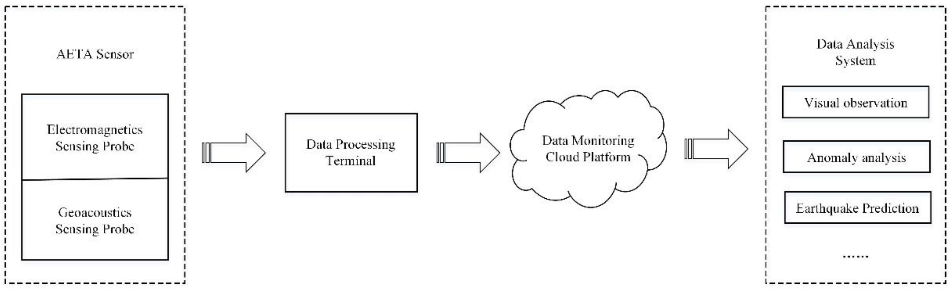
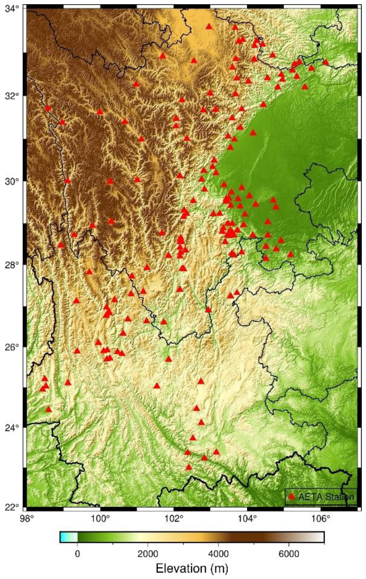
2. AETA System

Acoustic and electromagnetics to artificial intelligence (AETA) is a system designed by the IMS Laboratory of Peking University for earthquake monitoring and prediction. It consists of an underground signal acquisition probe, a ground data processing terminal, a monitoring cloud platform, and a data analysis system, as shown in Figure 1. The underground part contains electromagnetic and geoacoustic sensor probes, which are utilized to collect electromagnetic and geoacoustic signals in real time. First, the collected data are transmitted to the terminal with the function of data processing on the ground. Processed data are then received by the monitoring cloud platform through the network for further analysis by the researchers [14].

This article focuses on the anomaly analysis of an impending earthquake based on AETA electromagnetic data. The design of the AETA electromagnetic sensor is similar to that of the search-coil magnetometer instrument (IMSC) on the French DEMETER and that on the Chinese electromagnetic satellite, based on Faraday’s electromagnetic theory. The induced electromotive force obtained from the magnetic field changing in the vertical direction is inputted into the front-end signal processing circuit for amplification, and is then filtered and processed via digital-to-analog conversion (DAC). The processed signal passes through the back-end acquisition circuit, which has a strong processing speed, STM32F407 as the control unit, and a W5300 high-speed Ethernet communication interface chip as the data transmission module to meet the needs of real-time detection. The parameters of the electromagnetic sensor are as follows: the electromagnetic probe monitors 0.1 Hz~10 kHz, covering very low frequency and ultra-low frequency electromagnetic bands with a wide dynamic range of 0.1~1000 nT. The device has an 18-bit resolution, a sensitivity of >20 mV/nT@ 0.1 Hz–10 kHz, and a noise level of 0.1–0.2 pT/Hz@ (10 Hz–1 kHz). It has a low frequency sampling rate of 500 Hz and a full frequency sampling rate of 30 kHz [15].

So far, the IMS laboratory has installed more than 200 AETA devices nationwide, and 150 of them are in the regions of Sichuan and Yunnan (22° N–34° N, 98° E–107° E). The reason for this is that this area has high incidence of earthquakes, and more than 200 earthquakes with a magnitude of 3.5 or higher have occurred there since 2017, which requires further investigation. The distribution of all stations in Sichuan and Yunnan is shown in Figure 2.

3. Algorithm and Sample Extraction

3.1. Anomalies of Electromagnetic Signals before the Earthquake

The analyzed cases were selected from earthquakes (M. > 6.0) in the target area (22° N–34° N, 98° E–107° E) in recent years:

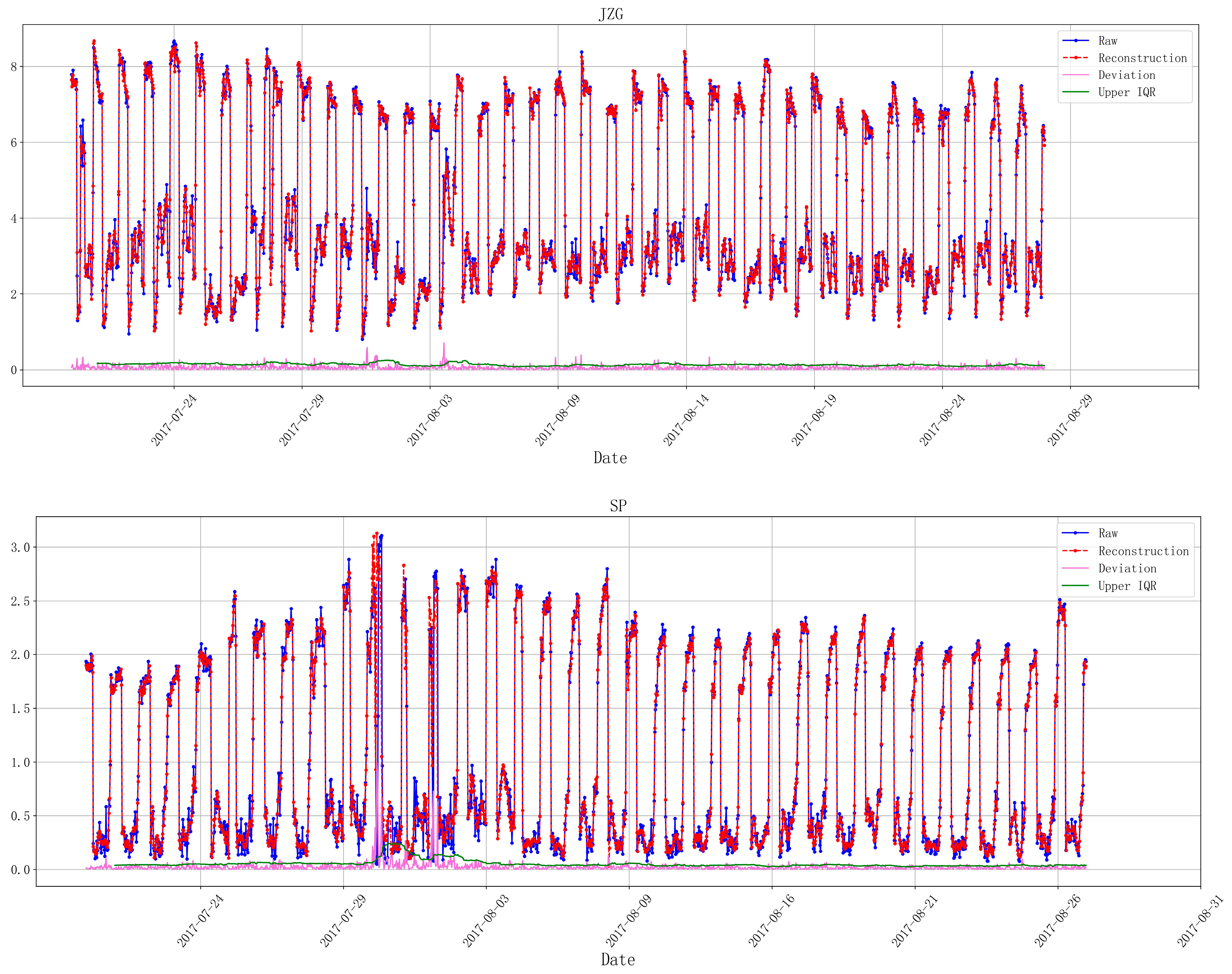
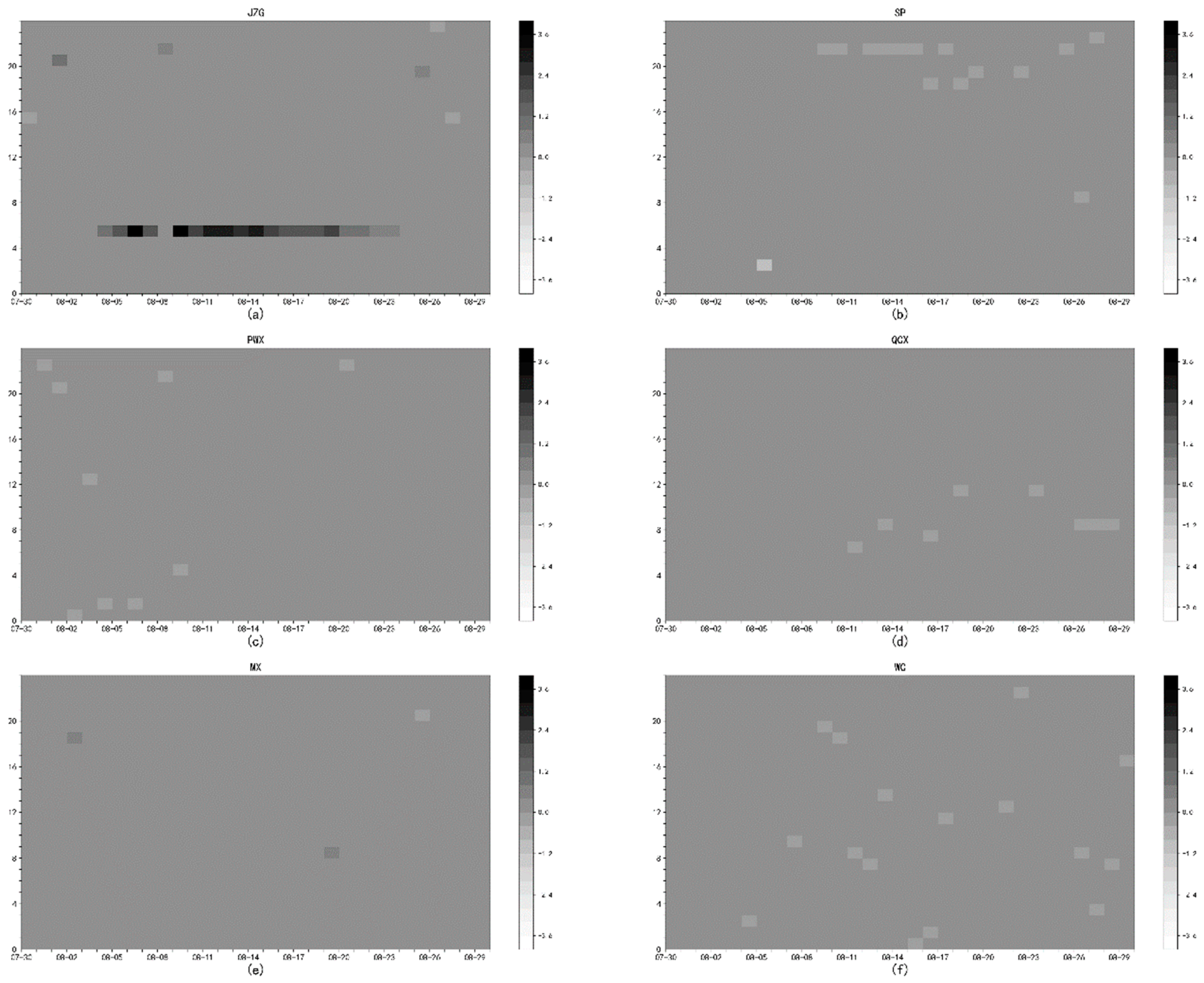
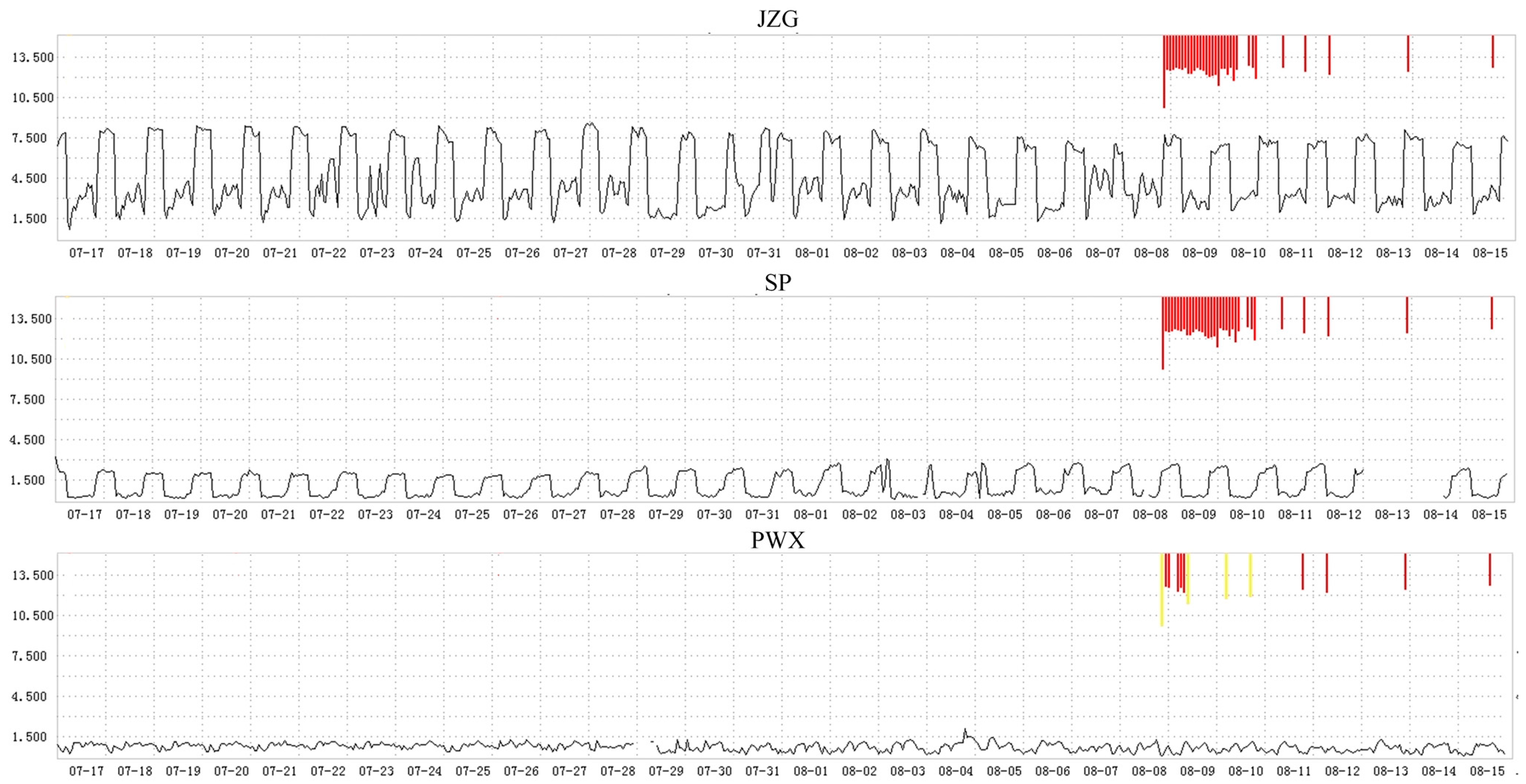
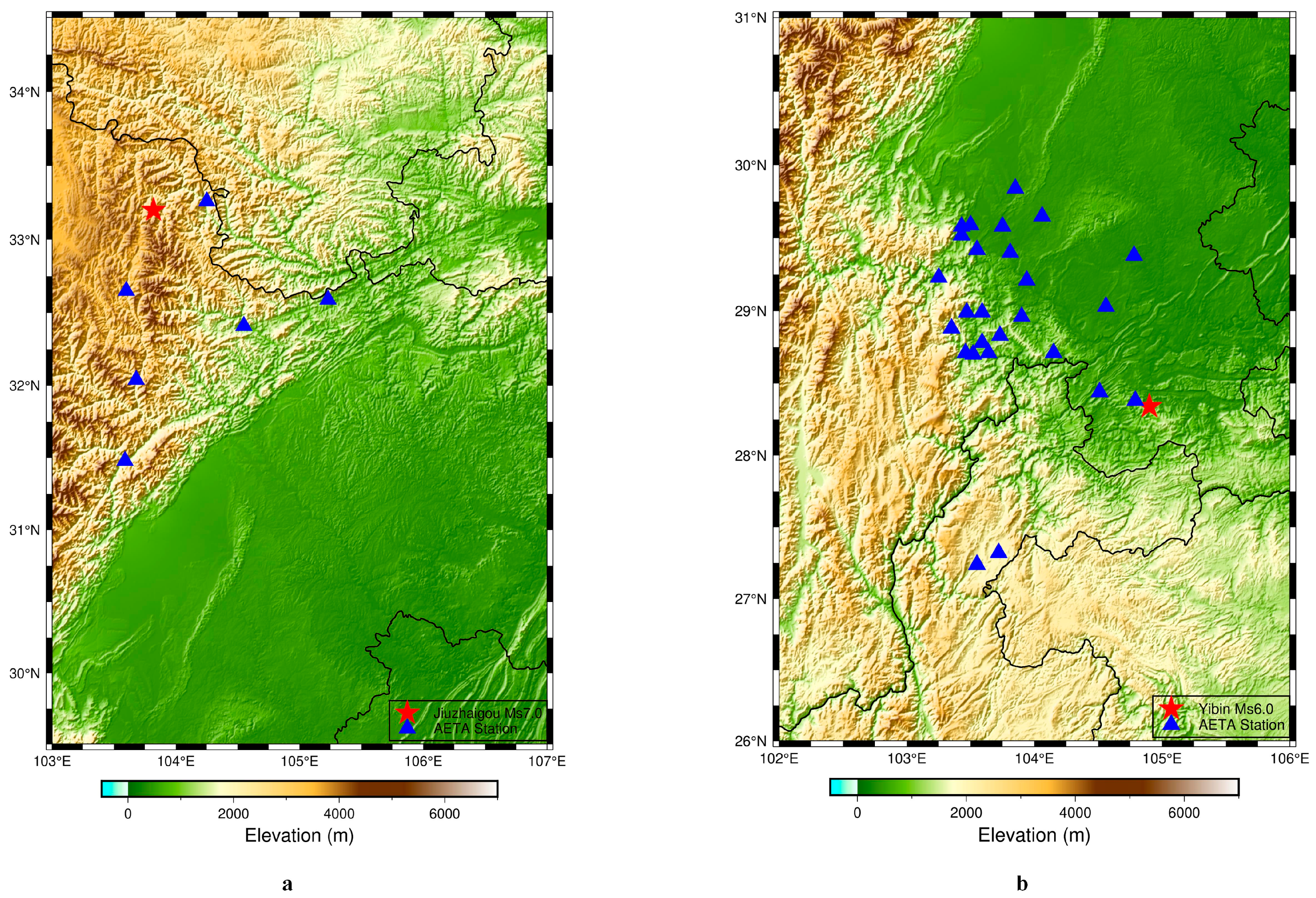
• On 8 August 2017, a magnitude 7.0 earthquake occurred in Jiuzhaigou County, Aba Prefecture, Northern Sichuan Province. Figure 3 shows the changes of the electromagnetic disturbance signal of the AETA stations near the epicenter;
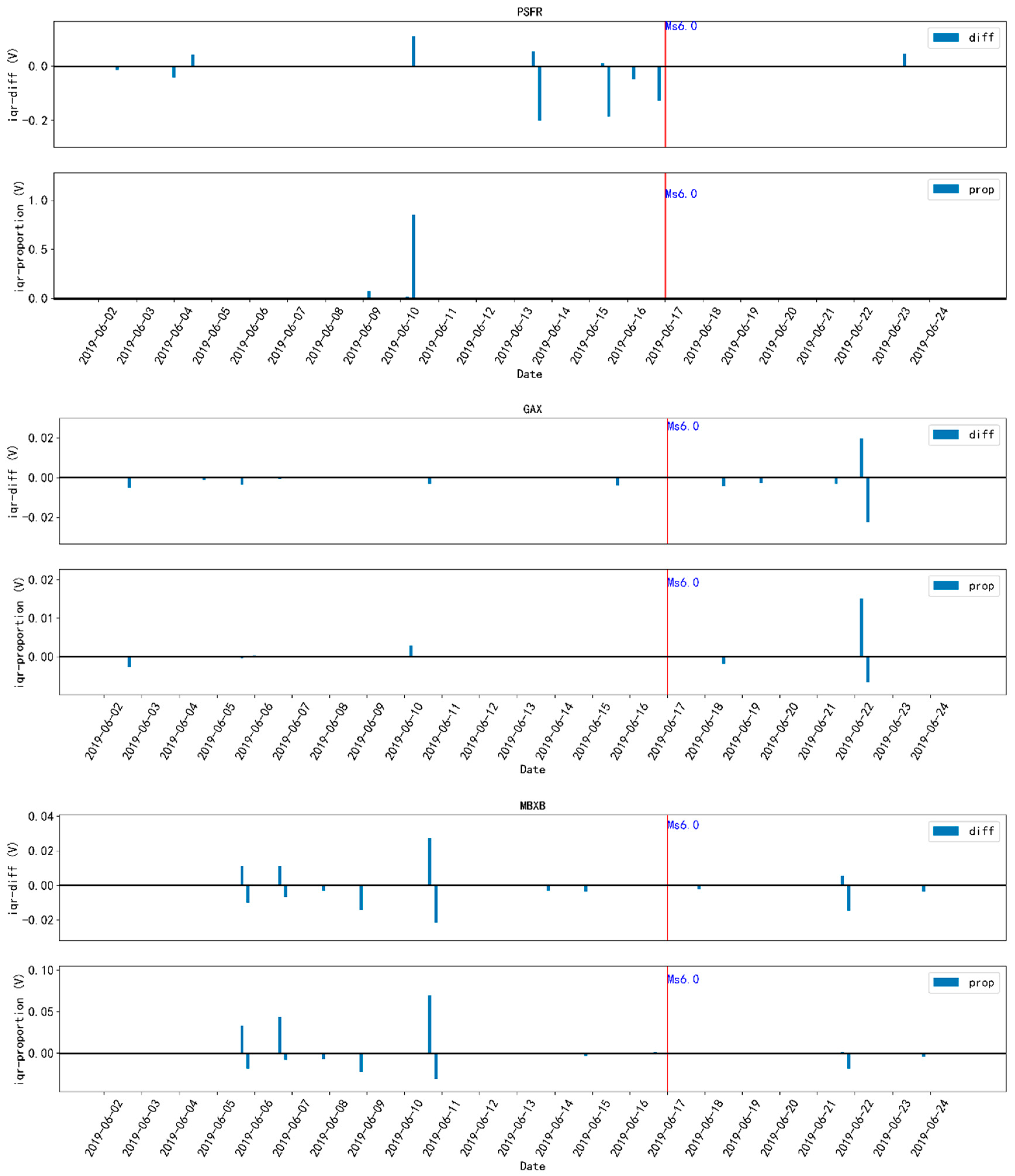
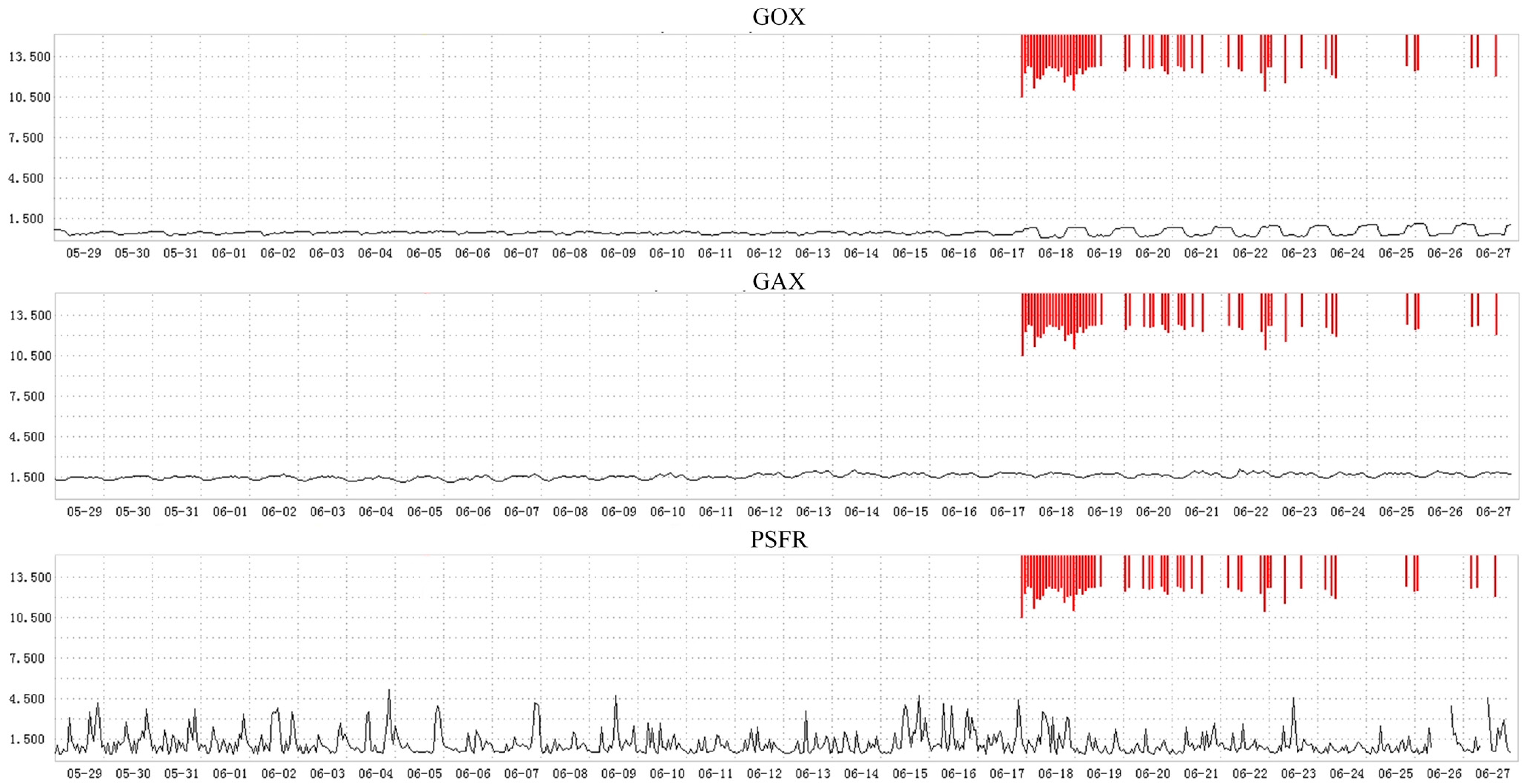
• On 17 June 2019, a magnitude 6.0 earthquake occurred in Changning County, Yibin City, Sichuan Province. Figure 4 shows the changes in electromagnetic disturbance signals of the AETA stations near the epicenter.

The red line at the top of the figure indicates the main shock and the aftershocks that followed.

It can be seen from Figure 3 and Figure 4 that there are some signal anomalies before the earthquakes, and we argue that the abnormal change is related to the occurrence of earthquakes. It is difficult to quantify such anomalies directly from manual observations, and there may be other undetectable changes in addition to this obvious information. These subtle anomalies mixed with abnormal disturbances are difficult to detect with the naked eye. Therefore, a lot of potentially abnormal information will be lost directly through simple observation. In order to discover the hidden information, we chose the LSTM autoencoder model to capture anomalies.

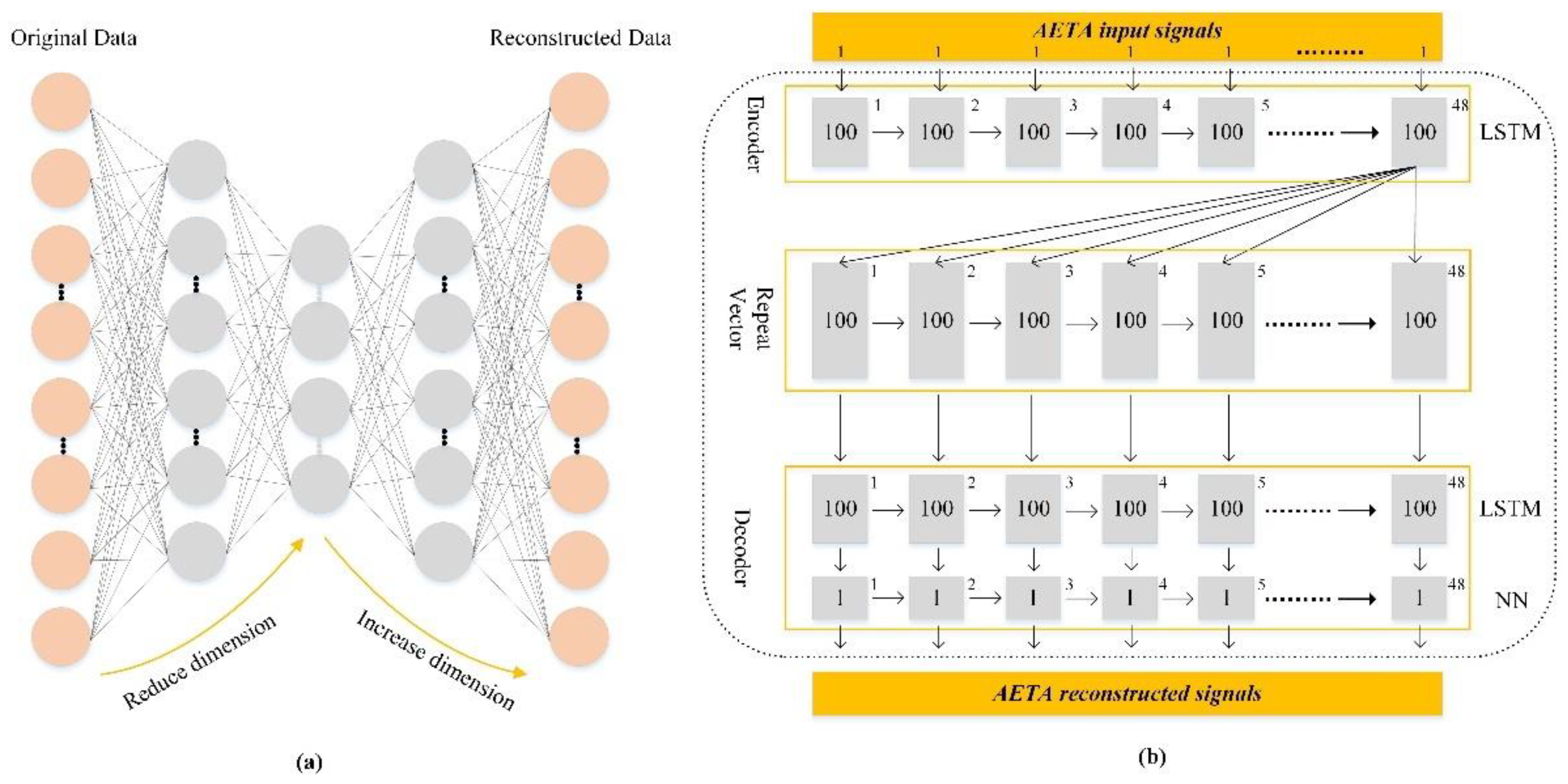
3.2. LAE and IQR Method

The autoencoder (AE) is an unsupervised neural network that aims to learn the reconstruction close to its original input. In general, it consists of two parts, an encoder network and a decoder network. The encoder reduces the dimension of the input vector $x\in {ℝ}^m$ and compresses it to the hidden vector $h\in {ℝ}^n(n<m)$, and then the decoder raises the dimension of the obtained hidden vector $h$ and maps it back to the original input space to obtain the reconstructed vector $\widehat{x}\in {ℝ}^m$. The difference between the original input vector $x$ and the reconstructed vector $\widehat{x}$ is called the reconstruction error $L\left(x,\widehat{x}\right)$ [16]. The autoencoder updates the weight of the network by minimizing the reconstruction error $L$:

$$L=\frac{1}{2}{\displaystyle \sum }_x\parallel x-{\widehat{x}\parallel }^2$$

(1)

The role of the autoencoder is not just to simply copy the input to the output. By constraining the latent space to have a smaller dimension than the input, i.e., $n<m$, the autoencoder is forced to learn the most salient features of the training data [17]. In other words, the autoencoder has a significant function in that it can find the regular or general pattern of the input data by reconstructing it.

Common autoencoders include the vanilla autoencoder [18], the convolutional autoencoder [19], the regularized autoencoder [20], and the LSTM autoencoder (LAE). As a form of sensor monitoring data, the AETA electromagnetic signal is a typical time series. The ability of LSTM to learn the patterns of long data makes it suitable for time series prediction or anomaly detection, and it is often used to capture the time dependence in multivariate data and determine whether data are out of distribution in a long time series. [21] In an LAE, both the encoder and decoder are LSTM networks. On the one hand, the fixed number of hidden units limit the model to learning the trivial mapping of the input; on the other hand, the same LSTM operation is performed recursively on the learned representation at any stage of decoding, which further hinders the model from learning the original mapping. This also explains why the LAE algorithm can achieve a reconstructed signal that presents almost all the input information but with a representation no better than the input [22]. The structure of the AE and LAE is shown as Figure 5.

The LAE created for AETA electromagnetic anomaly monitoring had two units corresponding to the encoding and decoding parts. The encoder consists of an LSTM layer with a size of 100 and a repeating module that is used to increase the dimension of the vector output by the former. There is also an LSTM layer and a flatten layer, which are used to transform the hidden layer vector from the encoder into reconstruction sequences with the same dimension as the input. The activation function applied for the LAE model was ReLU, which is based on a trial and error validation. We chose the Adam optimization as the optimizer and the mean square error (MSE) shown in Formula (1) as the loss function. The training data were shuffled for every epoch, and each station was trained for a sufficient number of epochs, about 200. The learning rate was initialized to 0.001. The weight decay was set to 0.005 and the dropout at 0.5, for all layers. The model stopped training data when the loss of validation set did not decrease for 50 consecutive generations.

Quartiles were always used to draw box plots in statistics; that is, all values were arranged from small to large and divided into four equal parts. The value at the position of the three division points is the quartile. Interquartile range (IQR) is a method in descriptive statistics that represents a set of data arranged in order, as well as the difference between the upper quartile ${\mathrm{Q}}_3$ and the lower quartile ${\mathrm{Q}}_1$ [23]. When the IQR method is utilized for the monitoring of abnormal phenomena, the outliers are usually defined as values less than ${\mathrm{Q}}_{lower}$ or greater than ${\mathrm{Q}}_{upper}$, as the following formula:

$$\mathrm{IQR}={\mathrm{Q}}_3-{\mathrm{Q}}_1$$

(2)

$${\mathrm{Q}}_{lower}={\mathrm{Q}}_1-1.5\mathrm{IQR}$$

(3)

$${\mathrm{Q}}_{upper}={\mathrm{Q}}_3+1.5\mathrm{IQR}$$

(4)

The reason for the robustness of IQR is that up to 25% of the data can become arbitrarily distanced without greatly disturbing ${\mathrm{Q}}_3$ or ${\mathrm{Q}}_1$ so that outliers cannot affect this standard [24].

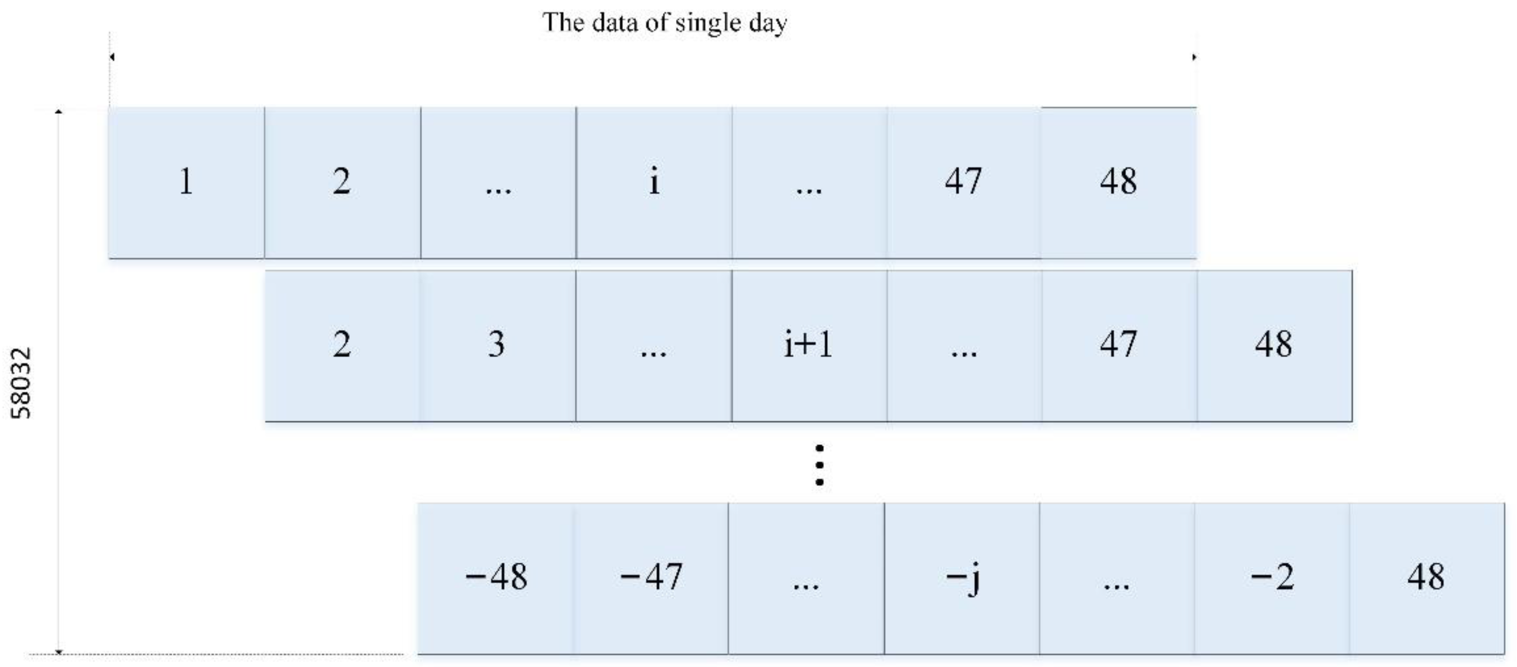
3.3. Sample Construction

The AETA signal is highly correlated with time, the quantity of data is large, and the information contained in a single point is insufficient. It is difficult for analysts who directly observe signals or utilize machine learning methods to process data to obtain valuable information, and they are likely to fall into a dilemma that they cannot resolve.

$$x=\frac{1}{n}{\displaystyle \sum }_{i=1}^n{x}_i$$

(5)

$n$ represents the total number of AETA electromagnetic data for half an hour.

We selected the electromagnetic disturbance data from 10 June 2017 to 10 December 2020, and, through the above formula, we obtained the average value of electromagnetic granularity data for 30 min. After that, the sliding window of the feature data processed from the AETA electromagnetic sensor was used as the input sequence, and the label had the same nature as the input with the size of 48, which was used to train the model more accurately, expand the training samples, and seek the abnormal information of the electromagnetic signal. Generally, since there are mostly samples with small magnitudes and too few instances with high magnitudes, it is necessary to consider how to handle class imbalance when performing earthquake prediction or magnitude classification tasks. However, the current study is an anomaly analysis of the AETA signal before the large earthquake, and there is no problem of sample imbalance. The sliding window method is shown in Figure 6, and a total of 58,302 samples were obtained.

4. Results

4.1. Seismic Case Analysis

During the period from 10 June 2017 to 10 December 2020, 92 earthquakes with magnitudes above 4.0 occurred in the target area (22° N–34° N, 98° E–107° E) selected in this study. Two earthquakes with a magnitude over 6.0 were chosen for this study through analyzing the outliers of the difference between reconstructed and original series to verify that the abnormal AETA data can reflect an impending large earthquake. The epicenter of two major earthquakes and nearby stations is shown in Figure 7.

4.1.1. Analysis of Jiuzhaigou M. 7.0 Earthquake

When the Jiuzhaigou M. 7.0 earthquake occurred, there were six effective AETA monitoring stations within 200 km of the epicenter.

Table 1. AETA Station within 200 km of the Jiuzhaigou epicenter.

No.	Station	Installation	Location	Epicenter Distance
—	Epicenter	—	33.20° N, 103.82° E	0
1	JZG	10 June 2017	33.25° N, 104.24° E	40 km
2	SP	12 June 2017	32.65° N, 103.60° E	64 km
3	PW	8 June 2017	32.41° N, 104.55° E	111 km
4	QC	7 June 2017	32.59° N, 105.23° E	147 km
5	MX	13 June 2017	31.69° N, 103.85° E	167 km
6	WC	13 June 2017	31.48° N, 103.59° E	192 km

shows the location and installation date of stations within 200 km of the earthquakes. Figure 8 shows the fitting effect of the LAE on the electromagnetic data of JZG and SP stations half a month before and one week after the earthquake. Figure 9 shows the curve fitted by the model on a specific day with or without anomalies, which can show the fitting ability of the model more clearly.

From Figure 8 and Figure 9, it can be seen that the LAE algorithm has an excellent ability to reconstruct time series data, which can fit the rising or falling trend of original data well. Figure 8 shows that both stations showed anomalous phenomena before the earthquake day (8 August). The anomalies gradually disappeared, and the deviation value tended to be stable after that day. In particular, the JZG station showed some abnormalities on 1 August and 3 August, and the SP stations showed strong abnormalities on 31 July and 1 August. At other times, the difference between the reconstructed and the raw value was within the normal range. From the detailed diagram of a single day, the model shows a strong fitting ability and can reconstruct the input data well, while it can no longer find the trend of the data, showing a larger deviation from the original input.

In order to enhance the robustness of the conclusion, we counted the number of outliers in all six stations before and after the earthquake, so that the anomalies of each station appear more intuitively in mathematical statistics. The abnormal points are defined as follows:

$$\Delta y=\{\begin{array}{cc}\hfill 0,& if \left|y-\widehat{y}\right|\le y_{upper}\hfill \\ \hfill \left|y-\widehat{y}\right|,& if \left|y-\widehat{y}\right|>y_{upper}\hfill \end{array}$$

(6)

where $y$ and $\widehat{y}$ represent the input and reconstructed data point, respectively. The deviation is $\Delta y$, and the IQR threshold value is $y_{upper}$. When $\Delta y>0$, the point belongs to an abnormal point. Otherwise, we consider the point as a normal point. If the point $\Delta y>0.7$, the point belongs to “outliers over 0.7” at the same time. The statistical results are shown in

Table 2. Station abnormal points before the Jiuzhaigou earthquake.

No.	Station	Abnormal Points	Outliers over 0.7	Total Points	Epicenter Distance
1	JZG	16	0	1152	40 km
2	SP	17	2	1152	64 km
3	PWX	12	0	1152	111 km
4	QCX	6	0	1152	147 km
5	MX	45	1	1152	167 km
6	WC	12	0	1152	192 km

.

It can be seen in Table 2 that, before the earthquake, about 2% of the points had anomalies. Among them, MX stations had the most total outliers, and, for the class of outliers exceeding 0.7, SP showed the most with two points. There were only six abnormal points in QCX with no value exceeding 0.7. In summary, before the Jiuzhaigou earthquake, the electromagnetic data of all the AETA stations showed abnormal disturbances, and that the number of anomalous points was irrelevant to the distance from the station to the epicenter. The reason may be that the electromagnetic waves received by different stations contain different seismic information that depends on geological structure when the electromagnetic data are propagated underground.

4.1.2. Analysis of Yibin M. 6.0 Earthquake

When the Yibin M. 6.0 earthquake occurred, there were more than 30 AETA monitoring stations within 200 km of the epicenter, 27 of which were operating normally and had robust data.

Table 3. AETA Station within 200 km of the Yibin epicenter.

No.	Station	Installation	Location	Epicenter Distance
—	Epicenter	12 December 2017	28.34° N, 104.90° E	0
1	GOX	13 January 2017	28.38° N, 104.79° E	11 km
2	GAX	13 March 2017	28.44° N, 104.51° E	39 km
3	YBYX	12 December 2017	29.03° N, 104.56° E	83 km
4	PSFR	12 December 2017	28.71° N, 104.15° E	84 km
5	ZGDA	21 August 2017	29.38° N, 104.78° E	115 km
6	MC	11 June 2017	28.96° N, 103.90° E	119 km
7	MBXB	11 October 2018	28.83° N, 103.73° E	126 km
8	MBMZ	12 October 2018	28.71° N, 103.64° E	129 km
9	JWX	8 June 2017	29.21° N, 103.94° E	134 km
10	MBJS	9 October 2018	28.78° N, 103.59° E	137 km
11	YJX	11 October 2018	28.70° N, 103.52° E	140 km
12	MB	16 October 2018	28.83° N, 103.54° E	143 km
13	YFZ	10 October 2018	28.71° N, 103.46° E	146 km
14	MBRD	12 October 2018	28.99° N, 103.59° E	146 km
15	DZB	21 August 2017	28.99° N, 103.47° E	157 km
16	ZT	21 August 2017	27.32° N, 103.72° E	162 km
17	SKH	1 August 2018	28.88° N, 103.35° E	162 km
18	JY	9 October 2018	29.65° N, 104.06° E	166 km
19	LSS	1 August 2018	29.58° N, 103.75° E	177 km
20	LSSW	9 October 2018	29.42° N, 103.55° E	177 km
21	LD	22 August 2017	27.24° N, 103.55° E	180 km
22	EB	11 April 2017	29.23° N, 103.25° E	188 km
23	GQZ	1 August 2018	29.52° N, 103.43° E	194 km
24	EMS	5 June 2017	29.59° N, 103.50° E	194 km
25	QSX	12 December 2017	29.84° N, 103.85° E	195 km
26	HWZ	1 August 2018	29.58° N, 103.43° E	198 km

shows the location and installation date of stations within 200 km of the earthquakes. Figure 10 shows the abnormal values after LAE fitting, which can more intuitively show the abnormality before and after the earthquake.

Figure 10 shows the statistical abnormal points at the PSFR, GAX and MBXB stations. Among them, $\mathrm{IQR}-\mathrm{Diff}$ refers to $\Delta y$ in Formula (6), and $\mathrm{IQR}-\mathrm{Prop}$ is the abnormal point obtained after we normalized the outlier and recalculated the IQR anomaly. We can see that some stations exhibited anomalies before the earthquake in the first and last pictures in Figure 10, and the middle section shows that some stations have abnormal data after the earthquake. The number or amplitude of the outliers obtained by Diff and Prop are similar, which further demonstrates the robustness of the method of extracting anomalies from the results of LAE processing. The IQR-Prop calculation method is defined as follows:

$$y_{min}=min\left(x_n\right)$$

(7)

$$y_{max}=max\left(x_n\right)$$

(8)

$$\overline{y}=\frac{\Delta y-y_{min}}{y_{max}-y_{min}}$$

(9)

$$\Delta y_{Prop}=\{\begin{array}{cc}0,\hfill & if \overline{y}\le {\overline{y}}_{upper}\hfill \\ \overline{y},\hfill & if \overline{y}>{\overline{y}}_{upper}\hfill \end{array}$$

(10)

where $x_n$ is the deviation series of LAE input and output, $\overline{y}$ is the normalized result of $x_n$, ${\overline{y}}_{upper}$ is the IQR anomaly threshold calculated after the sequence is standardized, and the anomaly value is $\Delta y_{Prop}$. The number of abnormal points at each station is shown in

Table 4. Station abnormal points before the Yibin earthquake.

No.	Station	Abnormal Points	Outliers over 0.7	Total Points	Epicenter Distance
1	GOX	35	5	1152	11 km
2	GAX	11	0	1152	39 km
3	YBYX	12	0	1152	83 km
4	PSFR	12	0	1152	84 km
5	ZGDA	6	0	1152	115 km
6	MC	15	1	1152	119 km
7	MBXB	17	0	1152	126 km
8	MBMZ	5	0	1152	129 km
9	JWX	12	0	1152	134 km
10	MBJS	9	0	1152	137 km
11	YJX	9	2	1152	140 km
12	MB	6	0	1152	143 km
13	YFZ	16	0	1152	146 km
14	MBRD	8	0	1152	146 km
15	DZB	14	0	1152	157 km
16	ZT	35	0	1152	162 km
17	SKH	15	0	1152	162 km
18	JY	4	0	1152	166 km
19	LSS	11	0	1152	177 km
20	LSSW	4	1	1152	177 km
21	LD	20	0	1152	180 km
22	EB	10	0	1152	188 km
23	GQZ	2	0	1152	194 km
24	EMS	16	3	1152	194 km
25	QSX	8	0	1152	195 km
26	HWZ	6	0	1152	198 km

.

4.2. Comparison with Principal Component Analysis (PCA) Method

PCA is a method widely used in the field of data mining and data analysis. It has the advantages of separating different signals and effectively identifying relatively weak signals and can be used for pre-earthquake electromagnetic disturbance analysis and total electron content (TEC) anomaly detection [25,26,27]. Therefore, we compared the results of the anomaly analysis of the Jiuzhaigou earthquake with those of the LAE using the PCA method. The results of the PCA are shown in Figure 11.

Figure 11 shows the thermogram of the abnormal values of each monitoring station from 1 August 2017 to 31 August 2017. The abscissa and the ordinate represent date and time, respectively. It can be seen from the figure that 5 days before the earthquake a continuous anomaly band with an increasing level of abnormality appeared at the JZG monitoring station at $5~6$ o’clock, and that the value of the abnormal points exceeded two in the 2 days before the earthquake, which was significantly higher than the other historical abnormal points in the background. The outlier point appeared at $21~22$ o’clock on the day of the earthquake, which means that the anomaly degree of the electromagnetic data at this time is greater than that at other times of the day. After the earthquake, the anomaly degree weakened generally, and the abnormal band appeared again at $5~6$ o’clock and lasted 15 days. However, other monitoring stations near the seismic epicenter have a relatively small degree of anomaly, and their thermograms do not constitute a continuous band anomaly.

In short, compared with the PCA method, the LAE can be used to observe the anomaly time and amplitude of the station more intuitively and conveniently. At the same time, in terms of the ability to identify seismic anomalies, the LAE method is robust. For example, for stations such as SP, it can capture anomalies not found by the PCA method. Therefore, the LAE is more suitable for anomaly analysis of AETA data before earthquakes.

5. Conclusions

In this study, the LAE and IQR methods were utilized to analyze the electromagnetic signals of the AETA stations near the Jiuzhaigou and Yibin epicenter. The results show that the electromagnetic signals of the AETA stations are obviously abnormal before the two earthquakes. First, the time, value, and number of abnormal points in stations at different geographical locations are not consistent, which is probably due to the difference of geological structure and the distance from the epicenter. The stations that were further away from the epicenter may show stronger anomalies than those closer. In general, there was obvious abnormal information about half a month before the earthquake. Secondly, the stations near the seismic epicenter generally exhibited outliers accounting for $2~4\%$ of the total data, and some stations had outliers with anomaly values exceeding 0.7 before the occurrence of a large earthquake, which shows that the electromagnetic anomaly of the AETA station has a certain correlation with the earthquake. Finally, comparing the methods of LAE and PCA through the case of the Jiuzhaigou earthquake, we found that the abnormal performance of the station is more common based on the LAE method, and that the ability to respond to abnormalities is also stronger and more intuitive. While the PCA method has good earthquake reflection performance at the JZG station, the performance of the other stations is not effective, which further proves the robustness of the LAE method used in this study.

In summary, the experiment in this study proves that the electromagnetic disturbance anomalies of the AETA station could imply an upcoming large earthquake, and that AETA electromagnetic signals can be regarded as a type of earthquake precursor. According to the experimental results, we believe that if $2\%$ of abnormal points appear in most monitoring stations within half a month, it means that a certain area has a higher risk of strong earthquakes.

In the future, we consider using a Generative Adversarial Networks (GAN) approach to generate several representative anomalous sequences. When the original signal matches these anomalous sequences, the system can automatically alert, which indicates that a certain area is facing the risk of high-level earthquakes. In addition, due to the complexity of actual seismic activity, it is difficult for us to directly estimate the geographical location of the epicenter from statistical values such as the number and amplitude of anomalous points. The use of AETA electromagnetic signals for earthquake prediction or early warning is awaiting further research in the future.

References

- Wyss, M.; Booth, D.C. The IASPEI procedure for the evaluation of earthquake precursors. Geophys. J. Int. 1997, 131, 423–424. [Google Scholar] [CrossRef]
- Kirschvink, J.L. Earthquake prediction by animals: Evolution and sensory perception. Bull. Seismol. Soc. Am. 2000, 90, 312–323. [Google Scholar] [CrossRef] [Green Version]
- Kulahci, F.; Cicek, S. Time-series analysis of water and soil radon anomalies to identify micro–macro-earthquakes. Arab. J. Geosci. 2015, 8, 5239–5246. [Google Scholar] [CrossRef]
- Han, P.; Hattori, K.; Hirokawa, M.; Zhuang, J.; Yoshino, C. Statistical analysis of ULF seismomagnetic phenomena at Kakioka, Japan, during 2001–2010. J. Geophys. Res.-Space Phys. 2014, 119, 4998–5011. [Google Scholar] [CrossRef]
- Sekertekin, A.; Inyurt, S.; Yaprak, S. Pre-seismic ionospheric anomalies and spatio-temporal analyses of MODIS Land surface temperature and aerosols associated with Sep, 24 2013 Pakistan Earthquake. J. Atmos. Sol.-Terr. Phys. 2020, 200, 105218. [Google Scholar] [CrossRef]
- Genzano, N.; Filizzola, C.; Hattori, K.; Pergola, N.; Tramutoli, V. Statistical correlation analysis between thermal infrared anomalies observed from MTSATs and large earthquakes occurred in Japan (2005–2015). J. Geophys. Res.-Solid Earth 2021, 126, e2020JB020108. [Google Scholar] [CrossRef]
- Feng, B.; Fox, G.C. TSEQPREDICTOR: Spatiotemporal Extreme Earthquakes Forecasting for Southern California. arXiv 2020, arXiv:2012.14336. [Google Scholar]
- Paul, S.; Mishra, S. LAC: LSTM AUTOENCODER with Community for Insider Threat Detection. In Proceedings of the 4th International Conference on Big Data Research (ICBDR’20), Tokyo, Japan, 27–29 November 2020; pp. 71–77. [Google Scholar]
- Daehyung, P.; Hoshi, Y.; Kemp, C.C. A Multimodal Anomaly Detector for Robot-Assisted Feeding Using an LSTM-Based Variational Autoencoder. IEEE Robot. Autom. Lett. 2018, 3, 1544–1551. [Google Scholar]
- Hashimoto, S.; Yonghoon, J.; Kudo, K.; Takahashi, T.; Umeda, K. Anomaly Detection Based on Deep Learning Using Video for Prevention of Industrial Accidents. arXiv 2020, arXiv:2005.13734. [Google Scholar]
- Nguyen, H.D.; Tran, K.P.; Thomassey, S.; Hamad, M. Forecasting and Anomaly Detection approaches using LSTM and LSTM Autoencoder techniques with the applications in supply chain management. Int. J. Inf. Manag. 2021, 57, 102282. [Google Scholar] [CrossRef]
- Khan, M.A.; Kim, Y. Deep Learning-Based Hybrid Intelligent Intrusion Detection System. CMC-Comput. Mat. Contin. 2021, 68, 671–687. [Google Scholar]
- Kim, H.; Arigi, A.M.; Kim, J. Development of a diagnostic algorithm for abnormal situations using long short-term memory and variational autoencoder. Ann. Nucl. Energy 2021, 153, 108077. [Google Scholar] [CrossRef]
- Wang, X.; Yong, S.; Xu, B.; Liang, Y.; Bai, Z.; An, H.; Zhang, X.; Huang, J.; Xie, Z.; Lin, K.; et al. Research and Implementation of Multi-component Seismic Monitoring System AETA. Acta Sci. Nat. Univ. Pekin. 2018, 54, 487–494. [Google Scholar]
- Yong, S.; Wang, X.; Pang, R.; Jin, X.; Zeng, J.; Han, C.; Xu, B. Development of Inductive Magnetic Sensor for Multi-component Seismic Monitoring System AETA. Acta Sci. Nat. Univ. Pekin. 2018, 54, 495–501. [Google Scholar]
- Hinton, G.E.; Salakhutdinov, R.R. Reducing the dimensionality of data with neural networks. Science 2006, 313, 504–507. [Google Scholar] [CrossRef] [PubMed] [Green Version]
- Sepehr, M.; Sasan, M.; Nicholas, R.J. Unsupervised anomaly detection with LSTM autoencoders using statistical data-filtering. Appl. Soft. Comput. 2021, 108, 107443. [Google Scholar]
- Han, W.; Wang, G.; Tu, K. Latent variable autoencoder. IEEE Access 2019, 7, 48514–48523. [Google Scholar] [CrossRef]
- Geng, J.; Fan, J.; Wang, H.; Ma, X.; Li, B.; Chen, F. High-resolution SAR image classification via deep convolutional autoencoders. IEEE Geosci. Remote Sens. Lett. 2015, 12, 2351–2355. [Google Scholar] [CrossRef]
- Hong, C.; Chen, X.; Wang, X.; Tang, C. Hypergraph regularized autoencoder for image-based 3D human pose recovery. Signal Process. 2016, 124, 132–140. [Google Scholar] [CrossRef]
- Mallak, A.; Fathi, M. Sensor and Component Fault Detection and Diagnosis for Hydraulic Machinery Integrating LSTM Autoencoder Detector and Diagnostic Classifiers. Sensors 2021, 21, 433. [Google Scholar] [CrossRef]
- Nitish, S.; Elman, M.; Ruslan, S. Unsupervised Learning of Video Representations using LSTMs. In Proceedings of the ICML, Lille, France, 6–11 July 2015; pp. 843–852. Available online: http://proceedings.mlr.press/v37/srivastava15.html (accessed on 24 June 2021).
- Bollini, P.; Chisci, L.; Farina, A.; Giannelli, M.; Timmoneri, L.; Zappa, G. QR versus IQR algorithms for adaptive signal processing: Performance evaluation for radar applications. IEE Proc.-Radar Sonar Navig. 1996, 143, 328–340. [Google Scholar] [CrossRef]
- Yang, K.; Yuan, P.; Qin, C. Consider the IQR Law in the Detection of Outlier in Time Series Considering Skewness. J. Geod. Geodyn. 2015, 35, 793–796. [Google Scholar]
- Yim, U.H.; Hong, S.H.; Shim, W.J.; Oh, J.R.; Chang, M. Spatio-temporal distribution and characteristics of PAHs in sediments from Masan Bay, Korea. Mar. Pollut. Bull. 2005, 50, 319–326. [Google Scholar] [CrossRef] [PubMed]
- Lin, J. Two-dimensional ionospheric total electron content map (TEC) seismo-ionospheric anomalies through image processing using principal component analysis. Adv. Space Res. 2010, 45, 1301–1310. [Google Scholar] [CrossRef]
- Ansari, K.; Panda, S.K.; Jamjareegulgarn, P. Singular spectrum analysis of GPS derived ionospheric TEC variations over Nepal during the low solar activity period. Acta Astronaut. 2020, 169, 216–223. [Google Scholar] [CrossRef]