1. Introduction
Ambient Intelligence (AmI) consists of technologies integrated into the physical environment for providing users with assistive and predictive support seamlessly. It combines artificial intelligence and the Internet of Things (IoT) with the pervasiveness of smart objects. In AmI-enabled environments, IoT is evolving as an intermediary layer between hardware systems and applications that offer intelligent services to people [
1,
2]. IoT connects a variety of networked devices that are embedded with sensors, applications, and other technologies in order to communicate and share data with other devices and systems [
3]. With billions of time series data collected from IoT in AmI-enabled environments, effective data mining methods are necessary to address these data [
4]. Anomaly detection is a vital research issue in data mining. It aims to identify the significantly different data from the most observations [
5]. Therefore, applying outlier detection technologies to the IoT time series can save computing time and predict the risk in smart environments. For example, in transportation systems based on AmI, IoT, and vehicular edge computing (VEC), anomaly detection can help vehicular users know the road condition in advance and avoid time loss caused by traffic incidents [
6,
7]. The existing approaches focusing on the outlier detection on the time series are learning the prior knowledge using the supervised learning model [
8] or utilizing the statistical methods to compute the probability distribution of the data [
9]. The statistical methods require that the data has a normal distribution and detect the outliers based on the statistical indices. The supervised learning learns the patterns of inliers and outliers from the training datasets and fits the supervised learning models. However, the patterns of outliers are diverse, so that the models cannot learn the patterns of all types of outliers. To overcome this problem, we discover the correlation between the multiple IoT time series for anomaly detection.
Traffic incident detection is one of the critical research issues in smart transportation systems [
6,
7,
10,
11]. In this study, we focus on the traffic incident detection problem with multiple traffic time series data. In this regard, we pose the following research questions:
How to extract incident patterns from multiple traffic time series data? (Q1)
How to construct the model for detecting incidents from extracted patterns? (Q2)
How to demonstrate the efficiency of the model? (Q3)
To address the research questions, we propose a new method to detect traffic incidents by identifying the anomaly among multiple traffic time series data. The proposed system collects traffic data from roadside units and connected vehicles and then detects the traffic incidents from the collected data to help users avoid the incidents and save travel time. We identify the correlation among the traffic time series to construct the dynamic graph. The graph is a typical data structure that consists of the vertices and edges for representing the correlation among the multiple data. The sliding window is exploited to generate the time intervals, and each time interval can be represented by using the graph. The dynamic graph consists of these graphs in continuous time. The graph entropy quantifies the information of the graph, and we compute the similarity between two graphs based on the graph entropy. The graphs with similar entropy have a small distance in the embedding space, while the graphs with anomalies are far from the regular graphs. Therefore, they can easily be detected as anomalies. The key contributions of this study are summarized as follows:
We propose a new idea for incident detection by discovering the correlation among multiple time series to build the graph and exploit the correlation to calculate the entropy of the graph.
We present the definitions of graph similarity based on the graph entropy for estimating the similarity between the two graphs. Then, we introduce a dynamic embedding model with the graph similarity to cluster the graphs for traffic incident detection in vehicular networks.
We conducted the experiments on multiple traffic time series data simulated by the Simulation of Urban Mobility (SUMO) simulator. The experimental findings show that the proposed model outperforms the baselines and performs better on high traffic volume scenarios.
The rest of this paper has the following structure. In
Section 2, background and related work are offered.
Section 3 discusses the dynamic graph embedding model for detecting traffic incidents in road networks. In
Section 4, experimental settings and results are explained. In
Section 5, the conclusion is finally given.
2. Background and Related Work
This section summarizes the background and related work of the paper. We first introduce the background of Ambient Intelligence, Internet of Things, and Vehicular Edge Computing. Then, we summarize the technologies related to graph embedding and their applications. Finally, the recent technologies for traffic incident detection are organized.
2.1. Ambient Intelligence, Internet of Things, and Vehicular Edge Computing
AmI is the ensemble of technologies embedded in human environments to seamlessly offer assistance and prediction in various contexts through a human–computer interface [
1,
2]. Examples of AmI environments are smart homes [
12], connected vehicles [
13,
14,
15], healthcare services [
16], smart grid [
17], and smart cities [
18]. AmI technology realization is an interdisciplinary area that includes sensor networks, artificial intelligence, and human–computer interaction. IoT, which is an enabling technology for promoting the interconnection and exchange of data between heterogeneous objects in smart environments by creating a connectivity network between sensors, embedded devices, and human–computer interaction, serves as the cornerstone of AmI [
2,
3].
With the advancement of AmI and IoT, new automotive innovations, e.g., autonomous vehicles, smart navigation, and cooperative cruise control, are starting to make modern transportation systems safer and smarter [
3,
19,
20,
21]. The traditional technology-driven transportation systems are turning into data-driven intelligent transportation systems, which produce a large volume of data, contributing to increased communication, computing, and storage demands as well as stringent latency and network bandwidth capacity criteria. VEC is emerging as a promising approach to overcome these problems [
20,
21]. VEC drives efficient computing and storage capacities from distant clouds to the edges of networks near vehicular users, allowing low response time and decreased bandwidth usage. As shown in
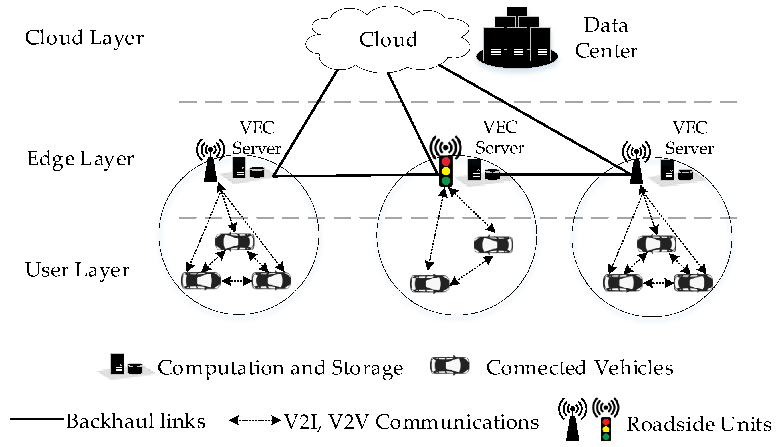
Figure 1, the architecture of VEC typically includes three layers: user layer (connected vehicles), edge layer (Roadside Units—RSU), and cloud layer (cloud servers). Connected vehicles have communicating capability, computing, and storage resources of their own. Connected vehicles can communicate via Vehicle-to-Vehicle (V2V) communications or with the RSU via Vehicle-to-Infrastructure (V2I) communications. RSU, operating as edge devices, are located near vehicles for real-time gathering, analyzing, and storing traffic information. Since vehicles have limited resources, they may shift latency-sensitive and compute-intensive tasks to edge devices, reducing delay and heavy workload on backhaul networks.
Since its inception, VEC has attracted a great deal of interest from scholars. Many works and surveys have examined different facets and applications of VEC, such as resource allocation [
22], traffic routing [
14,
15], and intersection control [
23]. Raza et al. [
20] discussed the VEC architecture’s technical issues and provided several recent solutions and future research challenges in the field. Liu et al. [
21] reviewed recent research in VEC by classifying the research topics, including task offloading, caching, information sharing, dynamic network control, privacy, and security.
2.2. Graph Embedding
Graph embedding captures the neighbor structure of vertices to map the vertices or graph into the embedding space. The graph embedding technologies are mainly divided into dimension-reduction-based methods, random walk-based methods, matrix-factorization-based methods, and neural network-based methods [
24]. With the development of deep learning, neural network-based models are proposed for the graph embedding issue. For example, a graph convolutional network (GCN) utilizes the convolutional kernels to extract the graph’s structure information and maps the vertices into the embedding space. The convolutional kernels extract the local structure’s features and compute the embedding vectors by reconstructing the graph. Jiang et al. [
25] combined spatiotemporal graph convolution network and recurrent neural network to construct a hybrid model for embedding the traffic graph to predict the traffic speed. The structural deep network embedding model [
26] defined two proximities for holding the local and global structures and computed the embedding vectors by using two autoencoders. The dynamic graph consists of the graphs in continuous-time intervals. Dynamic graph embedding maps the graphs into the embedding space based on similarity and temporality. Goyal et al. [
27] utilized the autoencoder to map the graphs into the embedding space and input the embedding vectors to the recurrent neural network to capture the temporal information for computing the final embedding vectors.
2.3. Traffic Incident Detection
Traffic incident detection is one of the key research topics in smart transportation systems [
6,
7,
10,
11]. The traffic incidents can be classified into five categories: accidents (e.g., collisions), road maintenance, hazardous weather, special events (e.g., Marathon), and obstacle vehicles. Existing methods are mainly based on deep learning technologies [
5]. Lin et al. [
6] proposed a traffic incident strategy based on the generative adversarial networks (GANs). The spatial and temporal features are extracted as variables from real traffic data. For feature engineering, the random forest was used to filter the features that are not important for detecting traffic incidents. To overcome the imbalance problem that the outlier samples are not enough, they utilized GANs to generate the data with the traffic incidents patterns. Support vector machine was used as the traffic incident detection method. This study utilized the datasets that have been labeled as outliers and inliers. However, the GANs model cannot generate the outlier patterns that were not in the datasets. Davis et al. [
7] constructed the transportation networks by using the temporal traffic data. The hybrid model combined with the long short-term memory (LSTM) and extreme value theory (EVT) was proposed to predict the traffic incident. LSTM is an improvement of the recurrent neural network. It drops the data that is not useful for predicting the traffic incident using the backward propagation algorithm. The EVT is applied to the loss function of the hybrid model. Via experiments, the proposed hybrid model achieves a better F1 score than the baselines. Since there is a possibility of overshooting in deep learning training, Hatri et al. [
10] used fuzzy logic to solve this problem. This method considers extracting the spatial and temporal information in the traffic data for incident detection. The results indicated that the proposed model could reduce the training time and the training loss. Zhang et al. [
11] collected the information from social media to detect the car accident from the traffic flow. The main idea is to collect the tweet contents about the traffic information. Then, they detect the accident by analyzing these tweet contents. However, they did not exploit the traffic flow directly for accident detection. Only using the information from social media to detect the accident lacks credibility. Unlike the existing works, we aim to develop a dynamic graph embedding model considering the correlation between the multiple traffic time series to detect incidents at intersections in the VEC environment.
3. Traffic Incident Detection Based on Dynamic Graph Embedding
Taking into account research questions Q1 and Q2, in this section, we describe the traffic incident detection based on the dynamic graph embedding. The main idea is to utilize the correlation between the multiple traffic time series to construct the graph where the nodes indicate the traffic flow and the weights of the edges is the correlation coefficient between two traffic flows. We set a sliding window to divide the multiple traffic time series into several time intervals and construct the dynamic graph. To quantify the graphs’ information, we calculate the graph entropy based on the correlation coefficient matrix. The dynamic graph embedding model is proposed to cluster the graphs. Since there is a stable correlation in the graphs without the traffic incident, the graphs with anomalies are far from the regular graphs. In this case, the abnormal graphs are discriminated and can be detected as a traffic incident.
3.1. Dynamic Graph Construction
Given two time series
x and
y, we can calculate their Pearson correlation coefficient [
28], which is formulated as
.
indicates that there is no correlation between them. For each time interval
, the correlation coefficient matrix of the dynamic graph
is formulated as
. The dynamic graph can be constructed by utilizing the correlations.
To measure the information of graphs, we calculated the graph entropy based on the information entropy [
29]. Given an event
x, the information of the event can be formulated as
where
indicates the probability of the event
x. The information entropy is described as the probability of the event times the information of the event, which is denoted as
. For the multiple independent events
, the information entropy is formulated as
where
X indicates the set of the events
and
N indicates the number of the events. To calculate the graph entropy, we first calculate the entropy of the vertex in the graph, which is calculated by using the weight of the edge.
Definition 1 (Vertex entropy). Given a graph where V indicates the set of the vertices and E indicates the set of edges. The entropy of the vertex is calculated based on the correlation between the vertices and , which is formulated as = where N indicates the number of vertices.
Then, we have to measure the information of the graph based on the vertex entropy. The vertex entropy measures the information of edges in the graphs. Supposing the vertex entropy is high, the vertex has a high correlation with the other vertices. It indicates that the corresponding time series plays an essential role in anomaly detection. To measure the graph entropy, we have to summarize the entropy of each vertex. The definition of graph entropy is as follows.
Definition 2 (Graph entropy). The graph entropy is calculated by summing the entropy of all vertices, which is formulated as . The dynamic graph entropy is described as the graph entropy at the time interval , which is formulated as .
3.2. Dynamic Graph Embedding
Dynamic graph embedding is utilizing the nonlinear function to learn the representation for mapping the graphs into the embedding space, where is the graph at the time intervals and is the embedding vectors of the graph . In this study, the graph G includes two elements which are correlation coefficient matrix and the graph entropy formulated as . The object of the dynamic embedding is clustering the graphs based on the similarity. It requires that the dynamic graph embedding considers the similarity of the neighbor structure between the graphs and considers the similarity of graph entropy. We define the graph similarity based on the correlation coefficient matrix and the graph entropy to solve this problem.
Definition 3 (Graph similarity). The graph similarity is described as the similarities of the neighbor structure and graph entropy, which is formulated as where indicates the similarity between the graphs and . The low similarity indicates that two graphs and are similar at the neighbor structure and graph entropy.
In this study, we used a graph proximity-based dynamic graph embedding model (DynGPE) to embed the graphs [
30]. Given a dynamic graph
,
and
indicates the graphs at the time interval
.
is the most similar graph with
. The embedding vector
is calculated at the embedding layer. The model consists of two autoencoders. The encoder maps the graph
into the embedding space by using the nonlinear function. The output of the decoder is to reconstruct the graph
. If the graphs
and
are close in the embedding space, the graph
is similar to the graph
. The inputs of the two autoencoders are the correlation matrices
and
and the hidden layers can learn the features from the correlation matrices by using the nonlinear functions
where
indicates the outputs of the
hidden layer and
and
indicate the weights and basis values at the
hidden layer, respectively. To make the functions nonlinear, we exploit the ReLU function as an activation function that is denoted as
[
31]. The input of the first hidden layer is the correlation matrix of the graph
, and the input of the next hidden layer is the output of the previous layer. The autoencoder reconstructs the input by reversing the nonlinear functions. Since the graph
is the most similar graph with the graph
on the neighbor, their embedding vectors are close in the embedding space.
Since the autoencoder learns the features by reconstructing the input, the similarity between the input and output is required to be small. We establish the loss function
to reduce the error between the input graph and the output where
T is the number of time intervals. To make two similar graphs on entropy close together in the embedding space, we establish the loss function
. The loss function
includes the embedding vectors of two graphs
and
so that the distance between them is reduced by optimizing the loss
. To avoid the overfitting, we add a regularization term, which is formulated as
where
L represents the number of layers and
W represents the weights. The joint loss function for optimizing the whole model is formulated as
3.3. Dynamic Graph Embedding-Based Traffic Incident Detection
In road traffic networks, the intersection areas are more susceptible to traffic congestion. Depending on the different root causes, traffic congestion can usually be divided into two types: (1) recurrent congestion and (2) nonrecurrent congestion [
32]. Recurrent congestion is caused by predictable phenomena, such as rush hours and holidays. Nonrecurrent congestion is produced by traffic incidents, for example, collisions, disabled cars, work zones, extreme weather conditions, and special events. Because of its unpredictable character, nonrecurring congestion produced by traffic incidents is more responsible for traffic delays than recurrent congestion in metropolitan areas. This work aims to develop an intelligent system that can use real-time, multiple time series from road traffic to determine an incident at the intersections.
To detect traffic incidents at the intersections, we utilize the installed RSU. Each RSU acts as a traffic controller, monitoring a specific intersection area for traffic incident detection in real time. V2V and V2I communications allow connected vehicles to perceive their driving surroundings and transmit the traffic data [
14,
15,
23]. When a connected vehicle enters the coverage area of the RSU, the vehicle broadcasts a message with its driving information (e.g., vehicle identification, current speed, waiting time, location, and timestamp). The RSU fuses the driving data of vehicles traveling in its coverage area and estimates the traffic flow parameters. Three fundamental characteristics in traffic flow theory are traffic volume, traffic speed, and occupancy [
6,
7,
10]. Although these parameters can be collected via inductive loop detectors (sensor-based) and cameras (vision-based) [
33], they are more correctly collected in real time under the VEC environment. In the context of the intersection area, the selected parameters are specified as follows.
Number of vehicles: The number of vehicles within the coverage area of the RSU. It represents the traffic volume characteristic of the traffic flow.
Mean speed (m/s): The average speed of all vehicles. It represents the traffic speed characteristic of the traffic flow.
Mean waiting time (s): The average time spent of all vehicles waiting to pass the intersection. The waiting time of a vehicle at the intersection is the consecutive time in which the vehicle was standing. It represents the occupancy characteristic of the traffic flow.
The RSU continuously collects the data and estimates three parameters, forming three data as time series. Then, we apply the dynamic graph embedding model to these time series for traffic incident detection. A graph is a typical data structure for modeling the items and their relationships. Therefore, it is used to build the correlation among the time series. Given a graph
,
V indicates the vertices in the graphs, and each vertex is a traffic time series. The weight value of the edge
E indicates the correlation coefficient between the two time series. The dynamic graph is composed of graphs in a continuous time. It records the evolution of the correlation among the traffic time series.
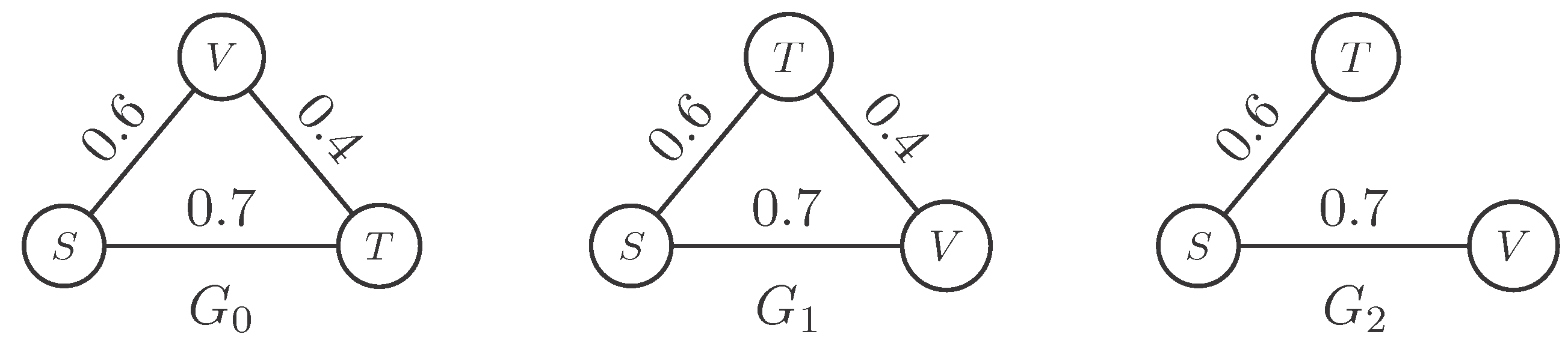
Figure 2 illustrates an example of the dynamic graph, where
S is the mean speed,
V is the number of vehicles, and
T is the mean waiting time. The weight of the edge indicates the correlation coefficient between two vertices, and
indicates the graph at the
time interval. Then, we calculate the entropy of the graph at each time interval. Next, we embed all graphs into an embedding space based on the graph entropy. Since there are multiple intersections and each intersection consists of a dynamic graph, we map the graphs of all intersections into an embedding space. In this way, the intersection with an incident is far from the most normal intersections, and we can detect the location and time of the incident.
4. Performance Evaluation
Regarding research question Q3, in this section, we compare the performance of the proposed method with other dynamic graph-based methods for detecting traffic incidents in a realistic road network.
4.1. Experimental Scenarios
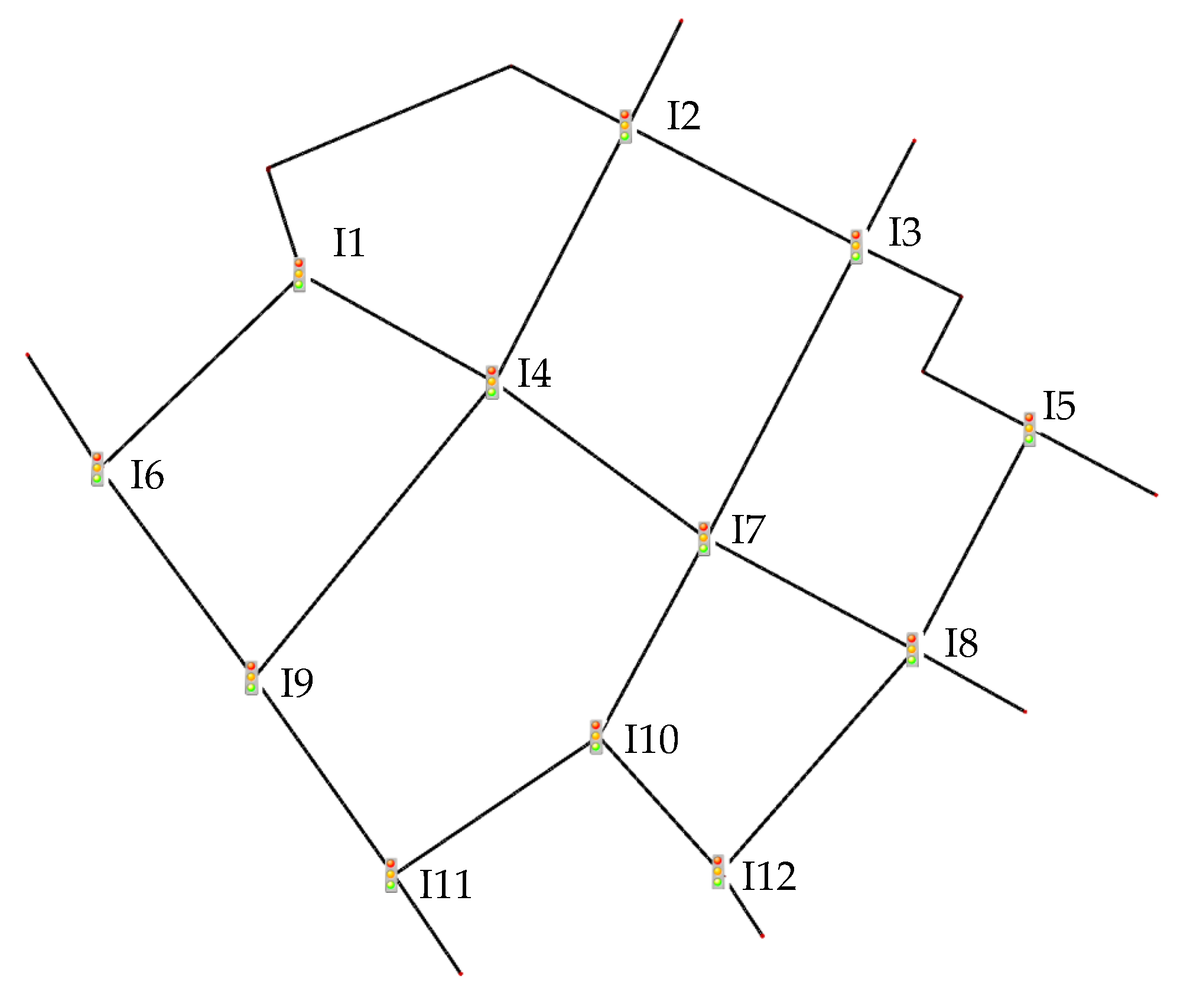
To generate the traffic data, we use the SUMO (
https://www.eclipse.org/sumo/ (accessed on 5 May 2021)), a well-known microscopic road traffic simulator [
15,
34,
35]. As shown in
Figure 3, the traffic scenario is a realistic road network at Lotte World, Seoul, South Korea, including 12 signalized intersections. It is obtained and converted from OpenStreetMap (
https://www.openstreetmap.org/ (accessed on 5 May 2021)) at the coordinates of
. A two-phase 90-s regulates the traffic light. Each intersection includes its RSU, and the connected vehicles can communicate and exchange traffic information to the RSU. The proposed method is implemented in the RSU to detect the incident at its coverage area.
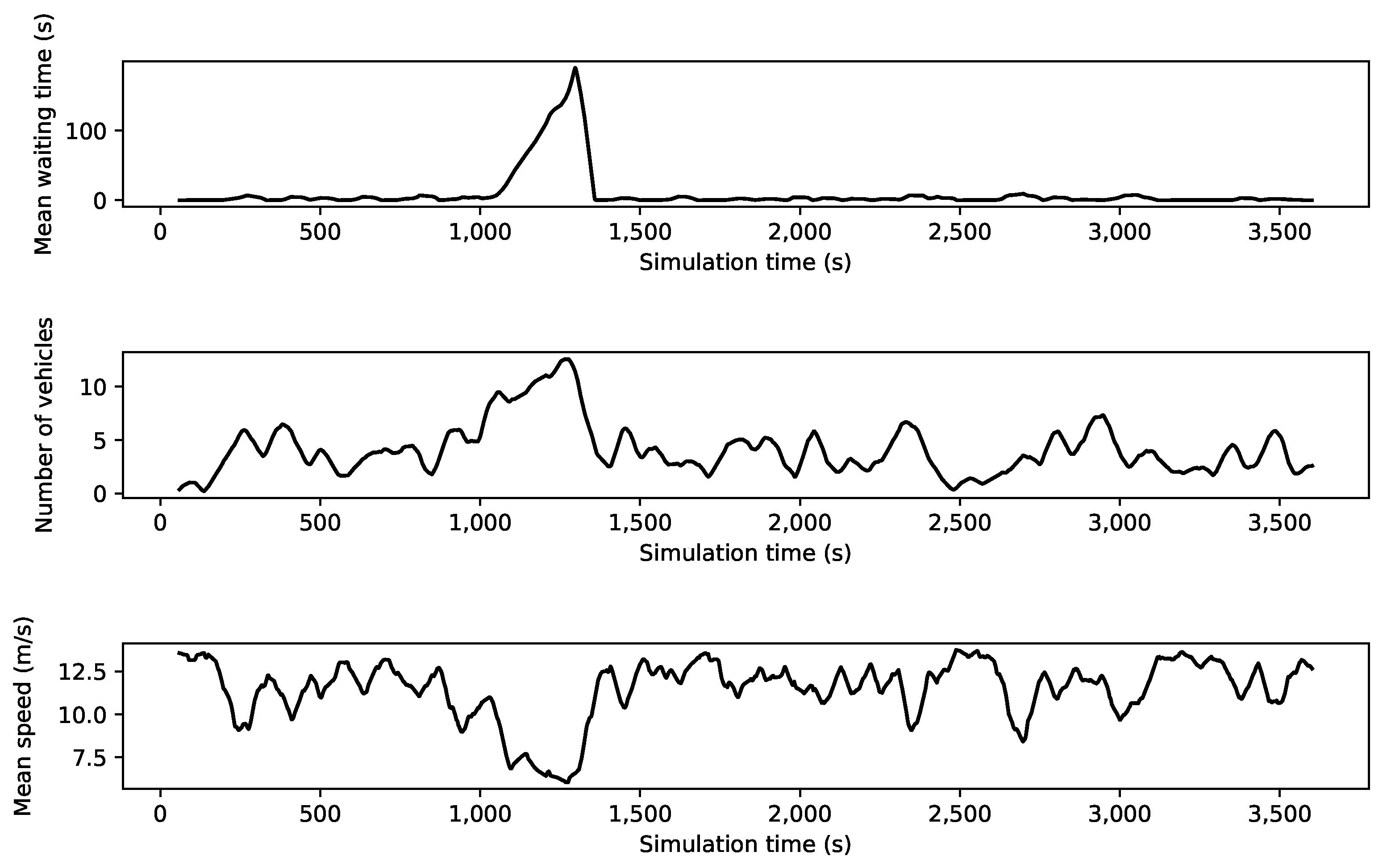
The vehicles are randomly generated by the randomTrips tool of SUMO with an arrival rate. As default, a binomial distribution is used to randomize the arrival rate, which is the number of vehicles generating per time unit. Three traffic volume scenarios are varying by the arrival rates. The number of vehicles generated is 500, 700, and 1000 vehicles, corresponding to low, medium, and high traffic volume scenarios. To simulate an incident, we stop some vehicles on a lane for a specific duration [
35], i.e., 300 s (5 min). The simulation time is 3600 s. The main parameters in the simulator are shown in
Table 1. The generated data includes features, such as mean waiting time, mean speed, and the number of vehicles in the form of time series data. An example of generated time series with the anomaly is illustrated in
Figure 4. In this generated data, traffic volume is medium, a traffic incident happens at the timestamp of 1000 at intersection
in the examined road network, and the incident duration is 300 s.
4.2. Methods and Performance Metrics
We compare the proposed method against the following models. Three models, which are based on the dynamic graph to vector architecture (Dyn2vec) for embedding the dynamic graph, are constructed using the autoencoder (Dyn2vecAE), recurrent neural network (Dyn2vecRNN), and autoencoder-based recurrent neural network (Dyn2vecAERNN) [
36]. Dyn2vecAE maps the dynamic graph into the embedding space by using an autoencoder. Dyn2vecRNN inputs dynamic graphs to the recurrent neural network to calculate the embedding vectors. Dyn2vecAERNN model utilizes the autoencoder to map the graphs into the low-dimensional space and inputs the embedding vectors into the recurrent neural network to learn the temporal features. In addition, we use the graph convolutional network (GCN) model as one of the baselines [
37].
This paper utilizes the sliding window to partition the traffic data into several time intervals. We select five slide windows with different sizes to divide the time series. The sizes of the slide windows are set as 200 s, 250 s, 300 s, 350 s, and 400 s. Given the incident period of 300 s, the reason for setting the sliding window with different sizes is that we want to observe the performance with three different cases, i.e., the size of the sliding window is smaller than, equal to, or is greater than the incident period.
Experiments are conducted with different traffic volumes and slide windows to obtain the performance with different parameters. We construct the ground truth as follows. The time intervals are divided by using the sliding window. If the time intervals do not include the incident timestamp, the time intervals are labeled as positive. The proposed model can then be evaluated by using the Accuracy (ACC) and F1 score as
where
represents the number of anomalies detected to be anomalous,
represents the number of nonanomalies detected to be nonanomalous,
represents the number of nonanomalies detected to be anomalous, and
represents the number of anomalies detected to be nonanomalous.
4.3. Results and Discussion
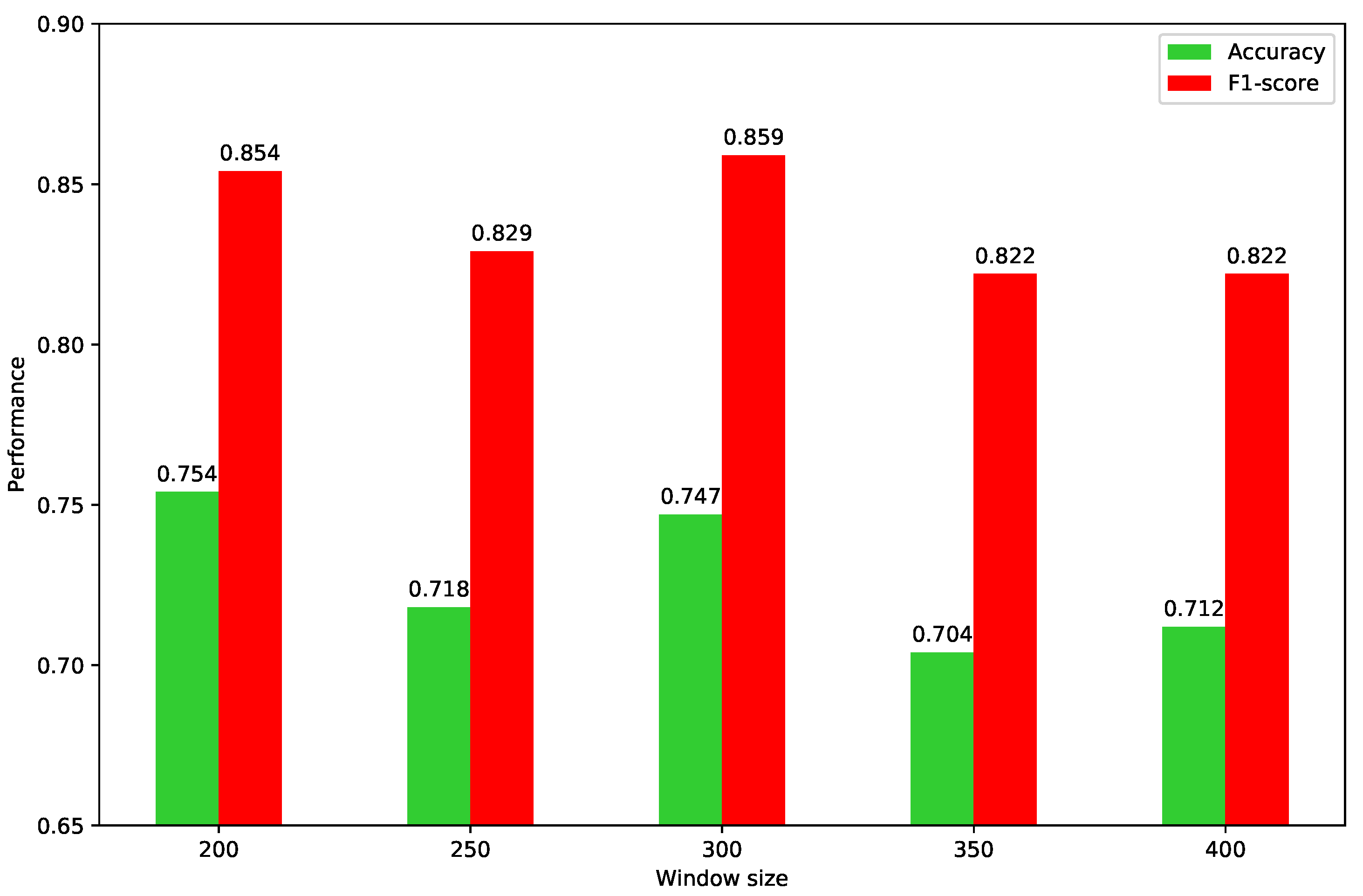
Figure 5 shows the results with different sliding windows of the proposed method. It achieves the best F1 score with a window size of 300. However, the accuracy with the window size of 300 is slightly lower than that of the window size of 200. It indicates that when the size of the sliding window is 300, there are graphs detected incorrectly. In terms of the F1 score, the results show that if the window size of the method equals the incident duration period, it achieves the best performance. This is because the large window sizes contain not only the abnormal interval but also some normal intervals. Therefore, the large window sizes affect the performance of the method. In contrast, the small window sizes cannot contain the whole abnormal time interval, so some abnormal patterns are ignored.
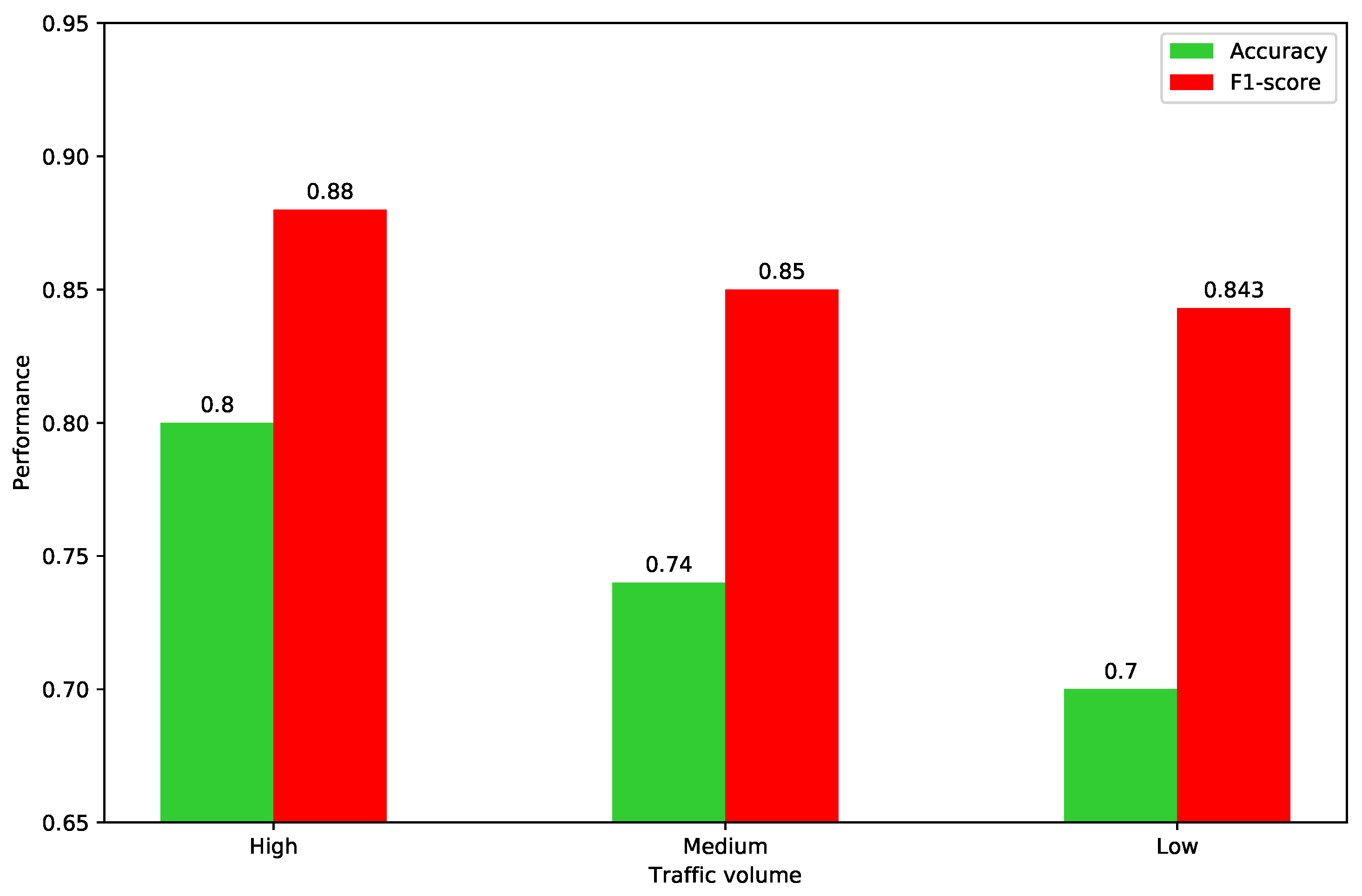
With the selected window size of 300, we conducted experiments to observe the performance with different traffic volumes. As shown in
Figure 6, with the decrease in traffic volume, the performance shows a downward trend. This is because in low traffic volume scenarios, the traffic flow is hardly interrupted, and traffic congestion may not occur even if traffic incidents happen. In other words, the mean speed, mean waiting time, the number of vehicles, and their correlation will not be significantly affected in the low traffic volume scenarios. Therefore, the accuracy of the incident detection in the low traffic volume scenarios is lower than that in the higher traffic volume scenarios.
Table 2 presents the results of the proposed method against other dynamic graph embedding methods. In all traffic volume scenarios, the proposed method has better results than the baselines by 14.5% and 18.1% on average with respect to F1 score and accuracy, respectively. GCN is a node embedding method that considers the neighbor structure of the vertices in the graph. In order to apply the GCN method to our research, we use two GCN models to build an autoencoder for calculating the embedding vector of each graph. According to the result, the performance of the GCN method is lower than the proposed method but outperforms the other methods. Dyn2vecAE model does not exploit the temporal information of the dynamic graph so that its performance is lower than that of the Dyn2vecRNN model. The combined model, Dyn2vecAERNN, considers the spatial and temporal information so that it achieves better results than the other two Dyn2vec-based models. Our method uses entropy as a measurement to embed the dynamic graph. Thereby, the graph with an abnormal entropy can be highly distinguished.
Table 3 shows the comparison results of the proposed method with different window sizes on the high traffic volume with respect to F1-score. According to the results, the proposed method exhibited the best performance by comparing with the baselines on all of the window sizes. The standard deviation of the proposed method is 0.012. It indicates that there is little affection with different window sizes. In addition, the window sizes of 300 and 350 achieved the best F1-score on our method. It indicates that we cannot find a window size to get the best performance of the proposed model. However, we can get a window size by calibrating the assigned time window, and the model can achieve a relatively good performance.
5. Conclusions
This work proposed a novel method for detecting traffic incidents on multiple traffic time series based on the dynamic graph embedding. The sliding window divides the time series into several time intervals, and the dynamic graph represents the correlation between the time series in each time interval. The graph entropy is exploited to measure the similarity between two graphs. Based on the graph similarity, we presented a dynamic graph embedding model for clustering the graphs. The object of the model is reducing the distance between two graphs, which are similar to the neighbor structure and graph entropy. In this case, if the neighbor structure and graph of two graphs are similar and their distance is short in the embedding space. The experiments were carried out with the traffic time series generated by the SUMO simulator. The experimental results demonstrated that the proposed model achieved better performance than the baselines by 14.5% and 18.1% on average with regard to F1 score and accuracy, respectively.
Some issues could be taken into account in future work. For enhancing the performance of the proposed method, we consider a hybrid model that combines the autoencoder and LSTM models to extract the temporal features for dynamic graph embedding. As the competing baselines are exclusively from the dynamic graph embedding models, the proposed method could be compared with other incident detection methods. For determining the right time window in the proposed method, we plan to utilize the wavelet transform to calculate the frequency domain of the multiple time series and divide the time series into several time intervals based on their frequency.
Author Contributions
Conceptualization, G.L., T.-H.N. and J.J.J.; methodology, G.L. and T.-H.N.; software, G.L. and T.-H.N.; validation, G.L. and T.-H.N.; formal analysis, G.L. and T.-H.N.; investigation, G.L. and T.-H.N.; resources, J.J.J.; data curation, G.L. and T.-H.N.; writing—original draft preparation, G.L. and T.-H.N.; writing—review and editing, J.J.J.; visualization, G.L. and T.-H.N.; supervision, J.J.J.; project administration, J.J.J.; funding acquisition, J.J.J. All authors have read and agreed to the published version of the manuscript.
Funding
This work was supported by the National Research Foundation of Korea (NRF) grant funded by the Korea government (MSIP) (NRF-2019K1A3A1A80113259, NRF-2020R1A2B5B01002207).
Institutional Review Board Statement
Not applicable.
Informed Consent Statement
Not applicable.
Data Availability Statement
Not applicable.
Acknowledgments
This research was supported by the Chung-Ang University research grant in 2020. Also, this work was supported by the National Research Foundation of Korea (NRF) grant funded by the Korea government (MSIP) (NRF-2019K1A3A1A80113259).
Conflicts of Interest
The authors declare no conflict of interest.
References
- Cook, D.J.; Augusto, J.C.; Jakkula, V.R. Ambient intelligence: Technologies, applications, and opportunities. Pervasive Mob. Comput. 2009, 5, 277–298. [Google Scholar] [CrossRef] [Green Version]
- Dunne, R.; Morris, T.; Harper, S. A Survey of Ambient Intelligence. ACM Comput. Surv. 2021, 54, 1–27. [Google Scholar] [CrossRef]
- Atzori, L.; Iera, A.; Morabito, G. The Internet of Things: A survey. Comput. Netw. 2010, 54, 2787–2805. [Google Scholar] [CrossRef]
- Cook, A.A.; Misirli, G.; Fan, Z. Anomaly Detection for IoT Time-Series Data: A Survey. IEEE Internet Things J. 2020, 7, 6481–6494. [Google Scholar] [CrossRef]
- Pang, G.; Shen, C.; Cao, L.; Hengel, A.V.D. Deep Learning for Anomaly Detection. ACM Comput. Surv. 2021, 54, 1–38. [Google Scholar] [CrossRef]
- Lin, Y.; Li, L.; Jing, H.; Ran, B.; Sun, D. Automated traffic incident detection with a smaller dataset based on generative adversarial networks. Accid. Anal. Prev. 2020, 144, 105628. [Google Scholar] [CrossRef] [PubMed]
- Davis, N.; Raina, G.; Jagannathan, K. A framework for end-to-end deep learning-based anomaly detection in transportation networks. Transp. Res. Interdiscip. Perspect. 2020, 5, 100112. [Google Scholar] [CrossRef]
- Baloglu, U.B.; Talo, M.; Yildirim, O.; Tan, R.S.; Acharya, U.R. Classification of myocardial infarction with multi-lead ECG signals and deep CNN. Pattern Recognit. Lett. 2019, 122, 23–30. [Google Scholar] [CrossRef]
- Jiang, Y.; Wang, Y.; Zhang, J.; Xie, B.; Liao, J.; Liao, W. Outlier detection and robust variable selection via the penalized weighted LAD-LASSO method. J. Appl. Stat. 2020, 48, 234–246. [Google Scholar] [CrossRef]
- Hatri, C.E.; Boumhidi, J. Fuzzy deep learning based urban traffic incident detection. Cogn. Syst. Res. 2018, 50, 206–213. [Google Scholar] [CrossRef]
- Zhang, Z.; He, Q.; Gao, J.; Ni, M. A deep learning approach for detecting traffic accidents from social media data. Transp. Res. Part C Emerg. Technol. 2018, 86, 580–596. [Google Scholar] [CrossRef] [Green Version]
- Costa, A.; Julián, V.; Novais, P. Advances and trends for the development of ambient-assisted living platforms. Expert Syst. 2016, 34, e12163. [Google Scholar] [CrossRef]
- Bennakhi, A.; Safar, M. Ambient Technology in Vehicles: The Benefits and Risks. Procedia Comput. Sci. 2016, 83, 1056–1063. [Google Scholar] [CrossRef] [Green Version]
- Nguyen, T.H.; Jung, J.J. Multiple ACO-based method for solving dynamic MSMD traffic routing problem in connected vehicles. Neural Comput. Appl. 2021, 33, 6405–6414. [Google Scholar] [CrossRef]
- Nguyen, T.H.; Jung, J.J. Swarm intelligence-based green optimization framework for sustainable transportation. Sustain. Cities Soc. 2021, 71, 102947. [Google Scholar] [CrossRef]
- Haque, A.; Milstein, A.; Fei-Fei, L. Illuminating the dark spaces of healthcare with ambient intelligence. Nature 2020, 585, 193–202. [Google Scholar] [CrossRef] [PubMed]
- Nguyen, T.H.; Nguyen, L.V.; Jung, J.J.; Agbehadji, I.E.; Frimpong, S.O.; Millham, R.C. Bio-Inspired Approaches for Smart Energy Management: State of the Art and Challenges. Sustainability 2020, 12, 8495. [Google Scholar] [CrossRef]
- Ohtsuki, T. A Smart City Based on Ambient Intelligence. IEICE Trans. Commun. 2017, 100, 1547–1553. [Google Scholar] [CrossRef] [Green Version]
- Guerrero-Ibanez, J.A.; Zeadally, S.; Contreras-Castillo, J. Integration challenges of intelligent transportation systems with connected vehicle, cloud computing, and internet of things technologies. IEEE Wirel. Commun. 2015, 22, 122–128. [Google Scholar] [CrossRef]
- Raza, S.; Wang, S.; Ahmed, M.; Anwar, M.R. A Survey on Vehicular Edge Computing: Architecture, Applications, Technical Issues, and Future Directions. Wirel. Commun. Mob. Comput. 2019, 2019, 1–19. [Google Scholar] [CrossRef]
- Liu, L.; Chen, C.; Pei, Q.; Maharjan, S.; Zhang, Y. Vehicular Edge Computing and Networking: A Survey. Mob. Netw. Appl. 2020. [Google Scholar] [CrossRef]
- Ning, Z.; Dong, P.; Wang, X.; Rodrigues, J.J.P.C.; Xia, F. Deep Reinforcement Learning for Vehicular Edge Computing. ACM Trans. Intell. Syst. Technol. 2019, 10, 1–24. [Google Scholar] [CrossRef] [Green Version]
- Bui, K.H.N.; Jung, J.J. Internet of agents framework for connected vehicles: A case study on distributed traffic control system. J. Parallel Distrib. Comput. 2018, 116, 89–95. [Google Scholar] [CrossRef]
- Chen, F.; Wang, Y.C.; Wang, B.; Kuo, C.C.J. Graph representation learning: A survey. APSIPA Trans. Signal Inf. Process. 2020, 9. [Google Scholar] [CrossRef]
- Jiang, M.; Chen, W.; Li, X. S-GCN-GRU-NN: A novel hybrid model by combining a Spatiotemporal Graph Convolutional Network and a Gated Recurrent Units Neural Network for short-term traffic speed forecasting. J. Data, Inf. Manag. 2021, 3, 1–20. [Google Scholar] [CrossRef]
- Wang, D.; Cui, P.; Zhu, W. Structural Deep Network Embedding. In Proceedings of the 22nd ACM SIGKDD International Conference on Knowledge Discovery and Data Mining, San Francisco, CA, USA, 13–17 August 2016; pp. 1225–1234. [Google Scholar] [CrossRef]
- Goyal, P.; Kamra, N.; He, X.; Liu, Y. DynGEM: Deep embedding method for dynamic graphs. arXiv 2018, arXiv:1805.11273. [Google Scholar]
- Edelmann, D.; Móri, T.F.; Székely, G.J. On relationships between the Pearson and the distance correlation coefficients. Stat. Probab. Lett. 2021, 169, 108960. [Google Scholar] [CrossRef]
- Soltangharaei, V.; Ai, L.; Anay, R.; Bayat, M.; Ziehl, P. Implementation of Information Entropy, b-Value, and Regression Analyses for Temporal Evaluation of Acoustic Emission Data Recorded during ASR Cracking. Pract. Period. Struct. Des. Constr. 2021, 26, 04020065. [Google Scholar] [CrossRef]
- Li, G.; Jung, J.J. Dynamic graph embedding for outlier detection on multiple meteorological time series. PLoS ONE 2021, 16, e0247119. [Google Scholar] [CrossRef]
- Moon, S. ReLU Network with Bounded Width Is a Universal Approximator in View of an Approximate Identity. Appl. Sci. 2021, 11, 427. [Google Scholar] [CrossRef]
- Afrin, T.; Yodo, N. A Survey of Road Traffic Congestion Measures towards a Sustainable and Resilient Transportation System. Sustainability 2020, 12, 4660. [Google Scholar] [CrossRef]
- Won, M. Intelligent Traffic Monitoring Systems for Vehicle Classification: A Survey. IEEE Access 2020, 8, 73340–73358. [Google Scholar] [CrossRef]
- Lopez, P.A.; Wiessner, E.; Behrisch, M.; Bieker-Walz, L.; Erdmann, J.; Flotterod, Y.P.; Hilbrich, R.; Lucken, L.; Rummel, J.; Wagner, P. Microscopic Traffic Simulation using SUMO. In Proceedings of the 2018 21st International Conference on Intelligent Transportation Systems (ITSC), Maui, HI, USA, 4–7 November 2018; pp. 2575–2582. [Google Scholar] [CrossRef] [Green Version]
- Smith, D.; Djahel, S.; Murphy, J. A SUMO based evaluation of road incidents’ impact on traffic congestion level in smart cities. In Proceedings of the 39th Annual IEEE Conference on Local Computer Networks Workshops, Edmonton, AB, Canada, 8–11 September 2014; pp. 702–710. [Google Scholar] [CrossRef]
- Goyal, P.; Chhetri, S.R.; Canedo, A. dyngraph2vec: Capturing network dynamics using dynamic graph representation learning. Knowl. Based Syst. 2020, 187, 104816. [Google Scholar] [CrossRef]
- Kipf, T.N.; Welling, M. Semi-supervised classification with graph convolutional networks. In Proceedings of the International Conference on Learning Representations (ICLR), Toulon, France, 24–26 April 2017. [Google Scholar]
| Publisher’s Note: MDPI stays neutral with regard to jurisdictional claims in published maps and institutional affiliations. |
© 2021 by the authors. Licensee MDPI, Basel, Switzerland. This article is an open access article distributed under the terms and conditions of the Creative Commons Attribution (CC BY) license (https://creativecommons.org/licenses/by/4.0/).


