Prediction of Transient Temperature Distributions for Laser Welding of Dissimilar Metals

Abstract

Distribution of temperature during the welding process is essential for predicting and realizing some important welding features such as microstructure of the welds, heat-affected zone (HAZ), residual stresses, and their effects. In this paper, a numerical model was developed using COMSOL Multiphysics of dissimilar laser welding (butt joint) of AISI 316L and Ti6Al4V thin sheet of 2.5 mm thickness. A continuous mode (CW) fiber laser heat source of 300 W laser power was used for the present study. A time-dependent prediction of temperature distributions was attempted. The heat source was assumed as a Hermit–Gaussian analytical function with a moving velocity of 120 mm/min. Both convective and radiant heat loss and phase change of the materials were considered for the analysis. In addition, variation of temperature-dependent material properties was also considered. The maximum and minimum temperature for the two materials at different times and the temperature in the different penetration depths were also predicted. It was found that the average temperature that can be achieved in the bottom-most surface near the weld line was more than 2400 K, which justifies the penetration. Averages of maximum temperatures on the weld line at different times at the laser spot irradiation were identified near 3000 K.The temperature fluctuation near the weld line was minimal and decreased more in the traverse direction. Scanning with a displaced laser relative to the interface toward the Ti6Al4V side reduces the maximum temperature at the interface and the HAZ of the 316L side. All of these predictions agree well with the experimental results reported in current literature studies.

1. Introduction

Titanium alloy of grade 5 (Ti6Al4V) and AISI 316L both have some excellent individual properties which make them suitable for different industrial applications. Ti6Al4V has low density, high specific strength, high erosion resistance, and high operating temperature [1], which make it suitable for aerospace and nuclear industries. However, AISI 316L is cost-effective and has high corrosion resistance. Dissimilar joining of Ti6Al4V with AISI 316L can be found in different industries such as in petrochemical, aerospace, and nuclear sectors. The main challenge of joining dissimilar materials [2,3,4] with differences in properties is the formation of intermetallic compounds (IMCs), which are brittle. There is also a high probability of crack formation due to residual stress generation. Solid-state joining processes such as diffusion bonding and friction stir welding process can be employed to join such materials to reduce IMC formation as it happens at low temperature. The major two drawbacks of the diffusion bonding process are large heat affected area and time-consumption. Friction stir welding is suitable for joining dissimilar metals; however, it even yields satisfactory outcomes for lap joint designs. The fusion welding process increases the chance of IMC formation as it has a high operating temperature [4,5]. It is very difficult to control the molten pool in the arc welding process and an expensive tantalum or vanadium sheet may be required to join them successfully [5]. High energy beam fusion welding using lasers can reduce HAZ and process time [5,6]. The formation of IMCs cannot be removed fully, but it can be controlled under optimal welding parameters.

A successful metal joint should be the priority for any welding process, but for realizing the process more deeply, numerical modeling is currently required. Laser welding [6,7,8] has become popular among other welding processes for joining both similar [9,10] and dissimilar materials [11,12]. The main reasons for its popularity are due to the higher precision and reduced HAZ zone during the joining process. Due to the complex nature of the laser welding process and the parameters involved in it, the numerical simulations are thereby desired for elucidating the joining process [13,14,15,16]. Past studies that modeled the laser welding process have aimed to predict the effects of the laser welding process on the resulting welded joints [16,17,18,19,20]. FE (finite element) simulation software such as ABAQUS, ANSYS, FLUENT, etc., has been used for 2D or 3D analysis of welding processes in different studies [17,18,19,20]. COMSOL [21,22] is one of the comparatively newer multiphysics software that can simulate the dynamics of the welding process. COMSOL is certainly a friendly choice for combining multiple physics, chosen for modeling and simulation purposes. The main complexity of simulation of the laser welding process is that all of the temperature-related parameters change in a very short span. Using ANSYS, Ranjbarnodeh et al. [23] predicted the temperature distribution for dissimilar welding of two different sheets of steel for the arc welding process. The maximum temperature obtained was more than 2100 °C. A nonsymmetric weld pool shape and temperature distribution was obtained. Akbari et al. [24] predicted the temperature distribution in Ti-6Al-4V welded joints using pulsed laser welding; their FE results matched their experimental data very well. Their results showed that decreasing the welding speed increased the peak value of temperature, while the width of the molten poll decreased. Kumar and Sinha [25] prepared a numerical model to predict the temperature distribution of two dissimilar steel alloys using ANSYS and validated their model against experimental temperature data collected using a K type thermocouple. Results reported that regardless of the disparity throughout thermal conductance of the components, the maximum temperature attained on the 304L portion of the varied weld-assemblage junction was higher than the maximal temperature obtained on the St37 carbon-steel portion. The maximal temperature variation of both materials lowers as backward from a welding-line [25]. Despite the fact that the source for heat energy is applied unevenly/uniformly throughout the numeric paradigm design, the temperature region curvature acquired for distinct laser-butt welding (DLBW) of 304L and St37 appears nonlinear and inherently unstable [25]. It was also discovered that the temperature profile both for identical and DLBW joints decreased dramatically close the weldment/welding-direction and then reduced marginally throughout the area farther aside toward a welding-line [25]. Attar et al. [26] used the FORTRAN programming language for predicting weld geometry, temperature contour, and strain distribution of copper and steel of 2 mm thickness joined by disk laser. They concluded that among all temperature-dependent properties, specific heat and thermal conductivity have a higher impact in numerical simulation. Li et al. [27] studied temperature field and molten pool dimensions with respect to the thickness of Ti6Al4V. The analysis indicated that the thin sheet decides an array for variables chosen throughout an attempt to attain an acceptable penetrating depth and breadth of melt pool [27]. Results indicated that the temperature and dimensions of such molten weld pool are significantly affected through altering a pulsed laser process variable. Reasonable weld bead quality was produced by selecting suitable process parameters. Because of the various cooling rates, the plate thickness now had the greatest effect on welding deviation. A comparatively low rate of cooling, caused by the thinner sheet producing a significantly greater temperature difference on the thin sheet, increasing pulsed laser power-beam source absorption as well as deviating a pool of molten metal against the thin sheet [27]. When the laser power density was reduced, the melting flow rate and temperature of the molten weld pool increased significantly more than when the other parameters were changed. The numerical simulations of temperature gradients matched the scientific evidential studies as well. Raising the weld speed to between 120 to 372 mm/min resulted in a significant reduction in the temperature of an adjoining proximity region of a molten weld zone between 280 and 98 °C for it and 0.1 cm thickness [27]. With 0.15 cm thickness, the temperature dropped from 224 to 68 °C. While the depth of a molten weld zone was the same across all thicknesses (0.1 and 0.15 cm), the breadth of a weld zone for 0.1 cm thickness was almost twice as large as the width of the melt pool for 0.15 cm thickness due to the orientation and slope of a weld zone toward the thinner layer [27]. Other research [28,29,30,31,32] assessed the transient temperature profile [20,33,34] of the weld materials utilizing finite element-based 3D models, considering various heat source models [35,36,37,38]. There are very few works with COMSOL on this and the combination is not considered much in the previous literature. In the present work, the thermo-physical properties of both materials (AISI 316L and Ti6Al4V) are considered to be temperature dependent and the interpolation method issued to obtain the properties in intermediate temperatures. Thereby, the transient (time dependent) 3D model in COMSOL is used to generate the geometry, mesh, isothermal contour, and temperature distribution along the weld line. Weld thickness is predicted for a fiber laser welding of dissimilar butt joints. For both AISI 316L and Ti6Al4V, temperature dependent material parameters such as heat capacity, thermal conductivity, and density are taken into account. Transient isothermal contours help to understand the heating and cooling phenomena during the process.

Using COMSOL Multiphysics, Jayanti et al. [39] developed a model for AISI 316L stainless steel welding using a pulsed laser beam as a heat source [21,22]. The thermal profiles were estimated in terms of surface temperature and isothermal contour, and hence, the temperature distribution was probed at radial directions from the centerline weld and on depth direction of the laser spot position. Their observations were discussed. Similarly, the thermal profile of the keyhole was predicted when the pulse was present and absent. The shape of the keyhole was viewed from both the top and front view [39]. The predicted keyhole was then compared with practical observation and results revealed that the temperature depended on the change in nonlinear physical properties such as density, thermal conductivity, thermal diffusivity, total enthalpy, inward heat flux, and Paclet number, which were plotted for the welding of AISI 316L stainless steel joint to study the change in microstructure and the mechanical properties [39].

Indhu et al. (2020) developed a (3D) axial symmetry model for laser welding of dissimilar materials in conduction welding mode [40]. To validate the model, experiments were carried out using a high power diode laser on dual phase steel and aluminum alloy in conduction mode. The model takes into account both the heat transfer and fluid flow. The temperature distribution of the weld pool and the weld pool geometry were contrasted against the empirical study observations [41,42,43].

The generation of the weld bead was aided by the laser energy density (LED). It was observed from the model that the peak temperature increased with escalated LED [40,41,42,43]. Owing to the increase in temperature, the amount of heat conducted into the material increased, which resulted in higher penetration depth. At the temperature distribution along YZ plane at a LED of 371 J/mm², the model generated a weld width of 6400 µm and a depth of 789 µm. At a lower LED of 297 J/mm², the weld width and penetration depth were reduced to 5410 µm and 393 µm [40,41,42,43].

The temperature profile was retrieved from the boundary by using six domain point probes positioned in the YZ plane along the weld’s cross section [40,41,42,43]. The temperature profile was depicted by the heating time and the cooling time for both cases at LED (371 J/mm² and 297 J/mm²). At higher LED (371 J/mm²), i.e., at lower scanning speed (8 mm/s), the laser remained in contact with the material for a longer time, which further resulted in increased heating time of 0.4 s and higher peak temperature of ~8200 K [40,41,42,43]. As the LED decreased (297 J/mm²), the heating time reduced to 0.25 s with a much lower peak temperature of ~7800 K. Results also revealed that another phenomenon that governed the weld width and the depth was the Marangoni convection force. Marangoni effect was the mass transfer that occurred due to the gradient in the surface tension in the molten weld pool [40,41,42,43].

The surface tension of the molten metal was increased with increase in temperature. The warmer liquid at point ‘a’ had lower surface tension and was pulled toward point ‘b’ [40,41,42,43]. The surface tension gradient along the molten pool caused an outward shear stress. As a result, the molten metal moved from the weld’s center to the pool’s margins before returning below the pool’s surface. At higher LED, the Marangoni convection increases, which result in larger weld width [40,41,42,43]. The influence of surface tension and gravitational forces were minimal when compared to the Marangoni convection forces acting in the weld [40,41,42,43].

In industries, welding of modern engineering materials including stainless steel and titanium alloys find a variety of applications due to the need to tailor the location of materials where a transition in mechanical properties, temperature, pressure, and/or performance in service is required. Owing to the wide range of uses with numerous advantages of the laser assisted welding process, it is essential to update, understand, and model before implementing industrial applications. As a result, the major goal of this research is to construct a finite element based three dimensional model for laser (CW) dissimilar welding of AISI 316L and Ti6Al4V with 2.5 mm thickness in butt weld configuration by using COMSOL Multiphysics codes. A three dimensional conical shape laser heat source model was considered. Weld geometry, mesh formation, transient temperature distribution prediction, development of temperature contours across the joint were accomplished. Individual specific and comparative temperature-distribution-based graphical representations of the two dissimilar welds (AISI 316L and Ti6Al4V) were plotted and further analyzed for efficacious comprehension and a better understanding of the thermal mechanisms involved in the welding process.

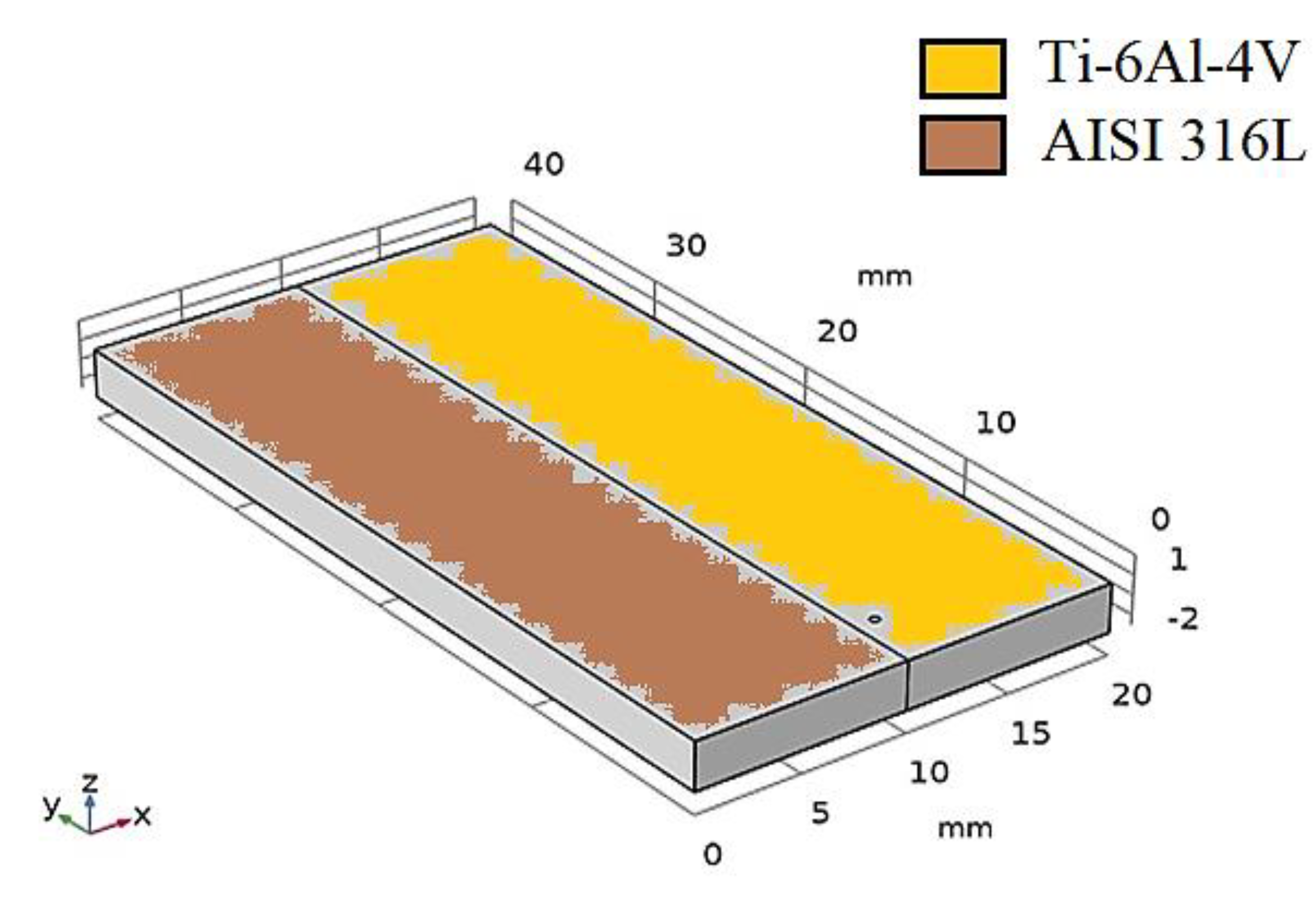
2. Definition of the Model

Two thin sheets of AISI 316L and Ti6Al4V with a thickness of 2.5 mm were used for laser welding in a butt joint design, as shown in Figure 1. The size of the sheets considered for modeling was 20 mm × 10 mm for both materials. A continuous mode (CW) fiber laser heat source of 300 W and laser beam radius of 200 μm was used for the present study. No filler material was used in this study. It was also assumed that the laser was focused on the welding line and moving at a constant speed of 2 mm/s. The transient study COMSOL was used for the prediction of the temperature fields in the welded joints. Thermophysical properties of both materials were considered to be temperature dependent and the interpolation method was used to obtain the properties for intermediate temperatures. The heat source plane was assumed as the z = 1 mm plane and the top surface of the sheets as the z = 0 plane. The work planes and work samples were considered as the union for simulation in design and evaluation prospective using COMSOL software.

For the present study, the following assumptions and features were used:

(a)

Radiation and convection heat loss from the surface are considered for modeling.

(b)

The ambient temperature is 298 K and the system is within good thermal isolation from the environment.

(c)

The change in phase during the process is also taken into account.

(d)

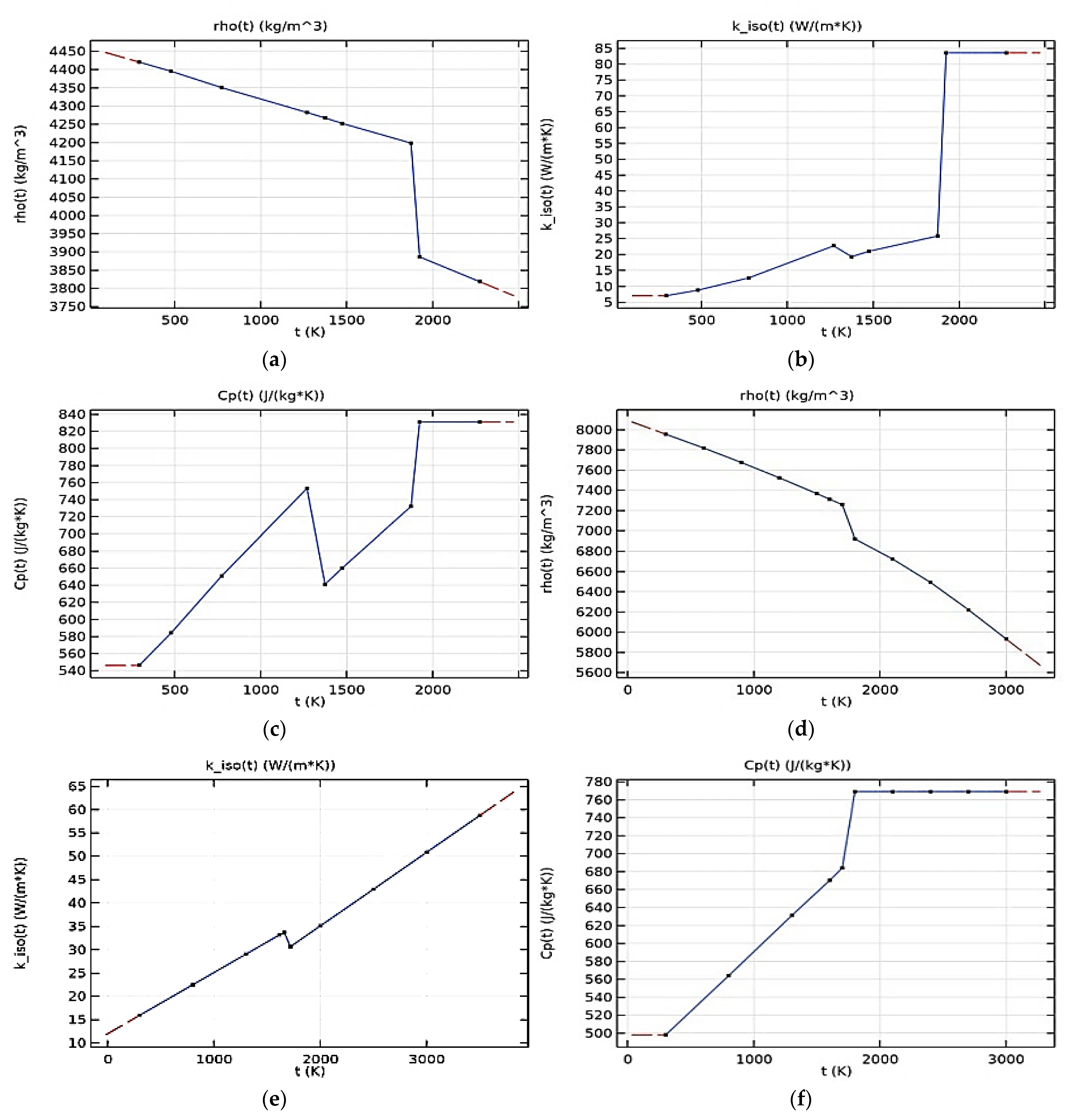
The thermo physical properties of the materials change with the change of temperature.

(e)

The position of the laser beam is vertical to the surface.

(f)

Latent heat during a phase change is considered for simulation. Latent heat for melting of Ti6Al4V and AISI 316L is 286 kJ/kg and 260 kJ/kg respectively.

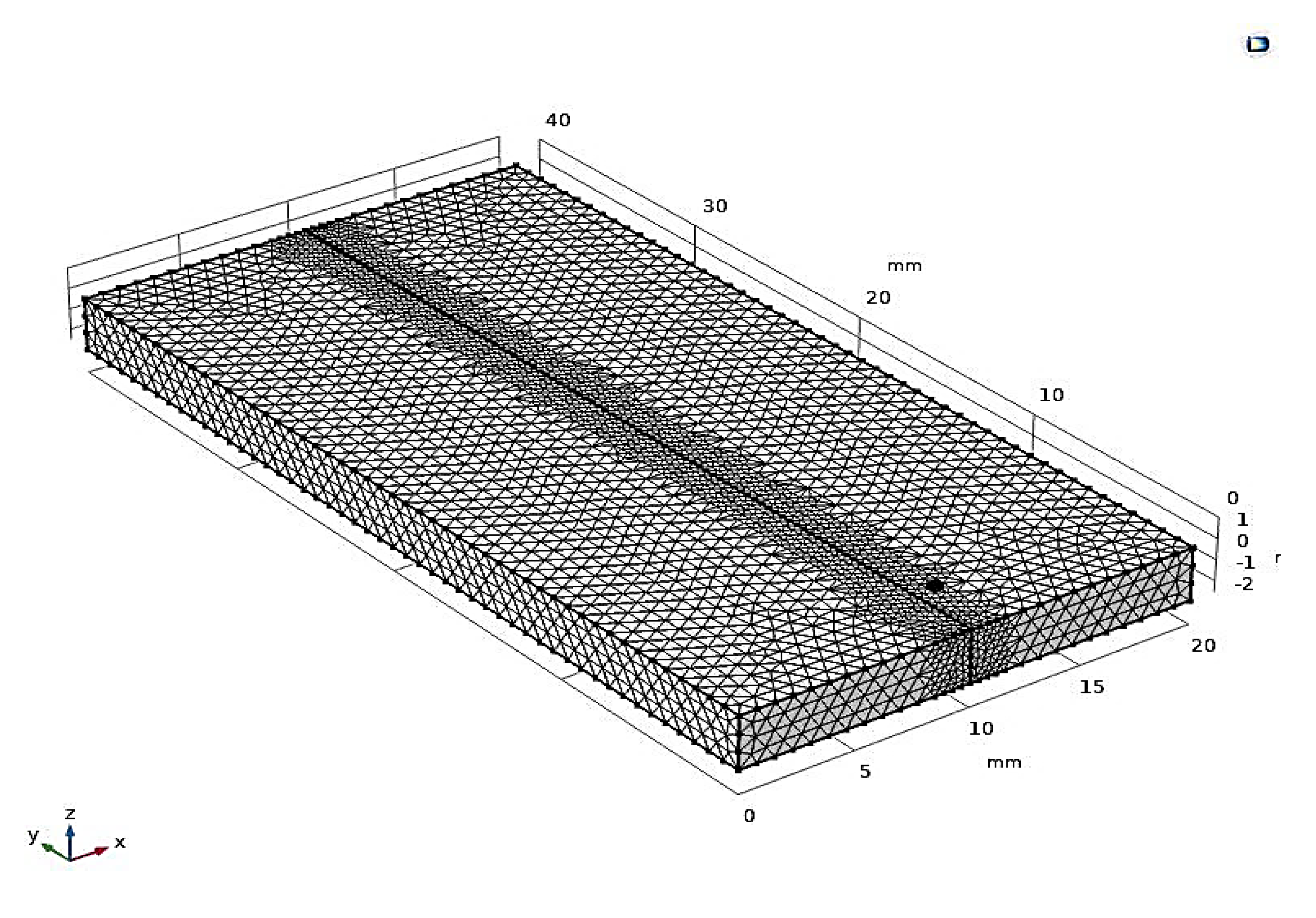
For modeling, the melting temperatures considered were 1703 K for AISI 316L and 1878 K for Ti6Al4V. In transverse electromagnetic (TEM00) mode, a three dimensional conical heat source was studied using the Hermit–Gaussian spatially distributed model [44,45]. As shown in Figure 2, for modeling the profile, a Hermit-Gaussian analytical function was used as it is one of the accurate profile model modes for laser welding. Previous research [46,47,48] that used this laser heat source model found that the results of numerical simulation agree well with experimental data, and provide a good match with the real weld pool shape with an error percentage as low as 7–8%, whereas other heat source models showed lower accuracy when compared against the experimental data [44,45,46,47,48,49]. In the fusion welding process, a heat source can be modeled as either a point heat source or line heat source. The mathematical expression of the heat source model follows:

$$an1=\exp \left[-\left\{\frac{{\left(a-a0\right)}^{2 }}{2\times sig{a}^2}\right\}-\left\{\frac{{\left(b-b0\right)}^{2 }}{2\times sig{b}^{2 }}\right\}\right]$$

(1)

The heat input equation of a moving heat source follows:

$$\begin{array}{l}Qin=Q0\times \left(1-Rc\right)\times Ac\times \left(\frac{1}{\pi \times sigx\times sigy}\right)\times an1\left(x,x0,sigx,y,y0,sigy\right)\\ \hspace{1em}\hspace{1em}\hspace{1em}\hspace{1em}\hspace{1em}\times \exp \{-Ac\times abs\left(z\right) \} \end{array}$$

(2)

The origin of the new coordinate frame was not static with respect to the old frame. It moves at a constant velocity with respect to the old frame:

$$d\left(t\right)=d0+t{v}_{no}$$

(3)

where, v_no and d0 are constant vectors. The vector v_no is the velocity of the origin of the new frame with respect to the old frame. d is the position vector of the origin of the new frame with respect to the old frame. The velocity of the origin of the new frame is the time derivative of d:

$$\frac{d}{dt}d=\frac{d}{dt}\left(d0+t{v}_{no}\right)=v_{no}$$

(4)

This vector gives the velocity of the origin of the new coordinate system with respect to the origin of the old coordinate system. In this model, only y axis velocity and t need to be considered in the new coordinate system for obtaining the boundary conditions. As long as t is not equal to 0, the position vectors with respect to one frame are different from the position vectors with respect to another frame.

At t = 0, d(0) = d0. The vector v_no has three components; Among them, d/dt(d_x) = 0, d/dt(d_y) = 0, and d/dt(d_y) = 2, which means that for any value of t, d_x(t) = d_x0 and d_z(t) = d_z0.

The starting position of the laser source is assumed to be 10 mm on x axis and 2 mm on y axis. The laser is moving at a velocity of 2 mm/s along the y axis and the total moving time for a sample is 17 s. The global parameters used for this model are given in

Table 1. Global parameters.

Parameters	Value	Details
x0	10 [mm]	x coordinate
y0	2 [mm]	y coordinate
Sigx	0.200 [mm]	Deviation along x
Sigy	0.200 [mm]	Deviation along y
Rc	0.001	Reflection coefficient
Ac	5 [1/cm]	Absorption coefficient
Q0	300 [W]	Laser power
L1	10 [mm]	Material size 1
L2	10 [mm]	Material size 2
LZ	2.5 [mm]	Thickness of the sheet
Time step	0.2	Time step for storing solution
End time	17 [s]	End time step
V	2.0 [mm/s]	Laser velocity
L	40 [mm]	Length of sheet

. The model arguments with upper and lower limit is mentioned in

Table 2. Model arguments with limits.

Arguments	Upper Limit	Lower Limit
a	(L1 + L2)	0
a0	x0	x0
Siga	Sigx	Sigx
b	2(L1 + L2)	0
b0	y0	y0
sigb	sigy	Sigy

.Temperature dependent thermal parameters (

Table 3. Temperature dependent properties with units.

Name	Value	Unit
Density	rho(T)	kg/m³
Thermal conductivity	k_iso(T)	W/(m·K)
Heat capacity at constant pressure	Cp(T)	J/(kg·K)

) are plotted from material properties [49,50]. These plots are important for obtaining the property values of intermediate temperatures within the working range, as shown in Figure 3. Some essential constant parameters are presented as well (

Table 4. Constant properties.

Name	Value
Convective heat transfer of air(h)	10 W/m2K
Emissivity(ε)	0.85

).

The model was developed with all the required parameters and simulated for the processing time step of 0.2 s as analyzed. The average isosurface temperature and the thermal contours across AISI 316L stainless steel and Ti6Al4V joint were obtained as output in order to estimate the temperature distribution during laser irradiation, similar to that of the welding process for specified parameters. Then, in order to probe temperature distribution in the direction of laser irradiation (z axis) and across the weld joint (x axis), the probe points were considered. From the probe points, the transient thermal responses in the two coordinates were probed at various points, since the thermal profiles as obtained from surface temperature and thermal contours were directly exposed the temperature distribution of entire weld joint.

3. Numerical Model

The FE model was built using the heat transfer option in the solid section of COMSOL Multiphysics. The simulation is based on the basic time dependent conduction equation for heat transfer in solids in three dimensions. The heat source moves along the y-axis at a velocity v(y) presented in the moving coordinate system, which ties to the moving heat source. Conduction takes a major role in transferring the heat which is applied by the laser beam to the particles of the working materials. Suitable boundary conditions are used to solve the transient heat conduction equation. Equation (5) makes it understandable that heat conduction within the materials depends on other parameters such as density, heat capacity, and thermal conductivity:

$$\rho c_p\frac{\partial T}{\partial t}+\rho c_p\left(\frac{dy}{dt}\right) \nabla T+\nabla ·\overrightarrow{q}=Q$$

(5)

$$\overrightarrow{q}=-k\nabla T$$

(6)

where ρ is the density, c_p is the specific heat at constant pressure, t is time, T is the temperature, k is the thermal conductivity, Q is volume heat rate and $\overrightarrow{q}$ is the heat flux vector.

Convection of heat between the surface and with the surroundings was considered as a part of heat lost during the laser welding process. Negligence of convection effect during simulation can be reflected as error when it is compared with any experimental data [51]. The heat loss from the top surfaces by natural convection was taken into account. The governing heat flux equation for convection is:

$$q_c=h\left(T-T_{ext}\right)$$

(7)

where h is convective heat transfer coefficient and T_ext is the surrounding temperature.

Heat loss in another form, i.e., radiation, was also considered during the simulation. Part of the total heat applied on the working surface is lost through radiation process. The accuracy of the model can be improved and the energy balance becomes more realistic by introducing these losses:

$$-\overrightarrow{n}·q_r=\epsilon \sigma \left(T_{ext}^4-T^4\right)$$

(8)

where $\overrightarrow{n}$ is normal outward vector, ε is the emissivity, and σ is Stefan’s constant.

Mesh Convergence Analysis

Meshing has a vital role in obtaining an accurate simulation model. COMSOL has a provision to make the meshing coarse or fine. Generally, the mesh at the vicinity and near the weld line should be finer than the rest of the two parts. Free tetrahedral meshing was chosen in the model builder as it is only fully an automatic 3D mesh generator and can be applied in any 3D geometry for various simulations with good accuracy. Figure 4 shows the free tetrahedron mesh formation of predefined extremely finer size with high optimization level. Near the weld line, the mesh was refined again for good simulation output. In the mesh used, there are 129,718 domain elements, 12,236 boundary elements, and 576 edge elements. Weld-bead element has an average quality of 0.8405. With a growth rate of 1.3, the mesh model has a maximum element size of 0.8 mm and a minimum of 0.008 mm.

4. Results

This section shows the computed transient temperature distribution by colored contour levels and graphs obtained from the simulated models.

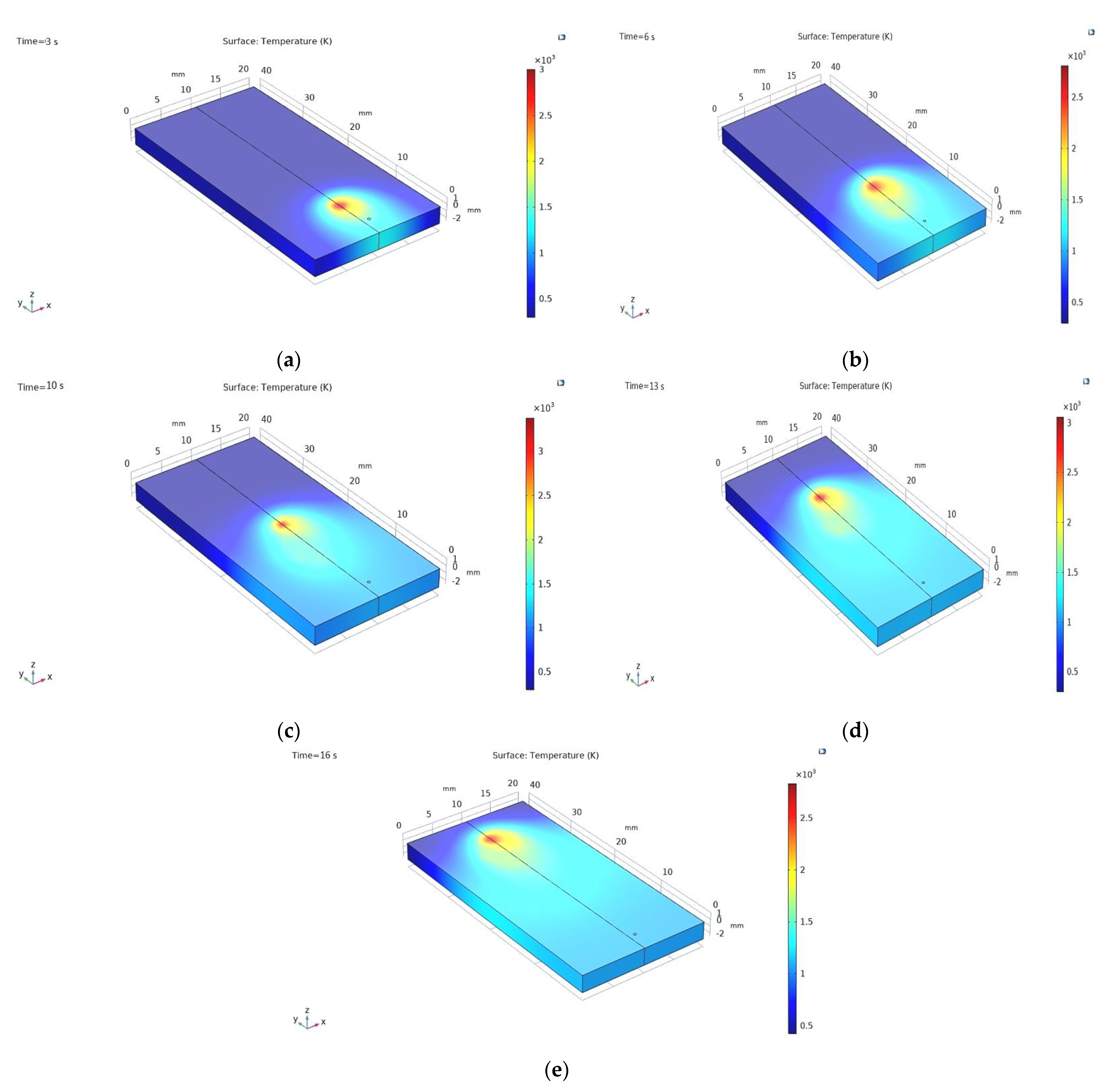
4.1. Temperature Propagation during the Welding

The study was conducted with a 300 W fiber laser heat source for two dissimilar materials having a thickness of 2.5 mm. The moving speed of the laser heat source was adjusted to 2 mm/s. Figure 5 shows temperature propagation of the upper surface on both sides from the weld line that can be predicted from these temperature distribution images. By the distinguishing colors of the image, it is possible to divide the weld bead zone into 4–5 zones: fusion zone, heat affected zone, softening zone, and base metal zone. Figure 5a–c shows large temperature gradients nearer to the heat source during the heating process. Figure 5d is for t =13 s and it basically indicates the heating process, but the cooling process had not begun at the areas farther from the heat source; i.e., the temperature gradient was still increasing. The last contour plot of Figure 5 (t = 16 s) clearly indicates the cooling process had started at the farther portion; i.e., temperature gradient began decreasing in those parts.

No very large fluctuation was observed in the temperature distribution along the weld line, as the heat supply was in continuous mode. The average value of fluctuation was nearer to 200 K. More fluctuation could be observed if the input mode was pulsed [39]. Farther from those in radial directions on both sides much less heat fluctuation was observed, which vanishes where no direct irradiation occurred. The temperature distribution of this part was similar for continuous and pulsed mode as direct irradiation was absent. However, no melting took place as a result of the temperature being less than that of the melting point for both materials. Thus, only a 4–5 mm of melt zone was observed in the model. This becomes clear from the probe points in the radial direction of joint, which revealed that, even at a distance of 5 mm from the weld, the temperature was near 1200 K—lower than the melting temperature of either material (Section 4.3).

The temperature distribution at the top and bottom weld bead showed that the higher temperature fluctuation throughout the top bead, which was due to the irradiation, remained well above the melting point of AISI 316 stainless steel and Ti6Al4V, which further ensured the full penetration welding for the entire joint. The predicted heat flow directions in terms of temperature gradient were oriented toward the solid region during laser–material interactions, and started decreasing while distance increased. This might be due to the heat loss by convection and radiation to the ambient surroundings, by conduction to the radial directions, and larger thermal gradient to the depth.

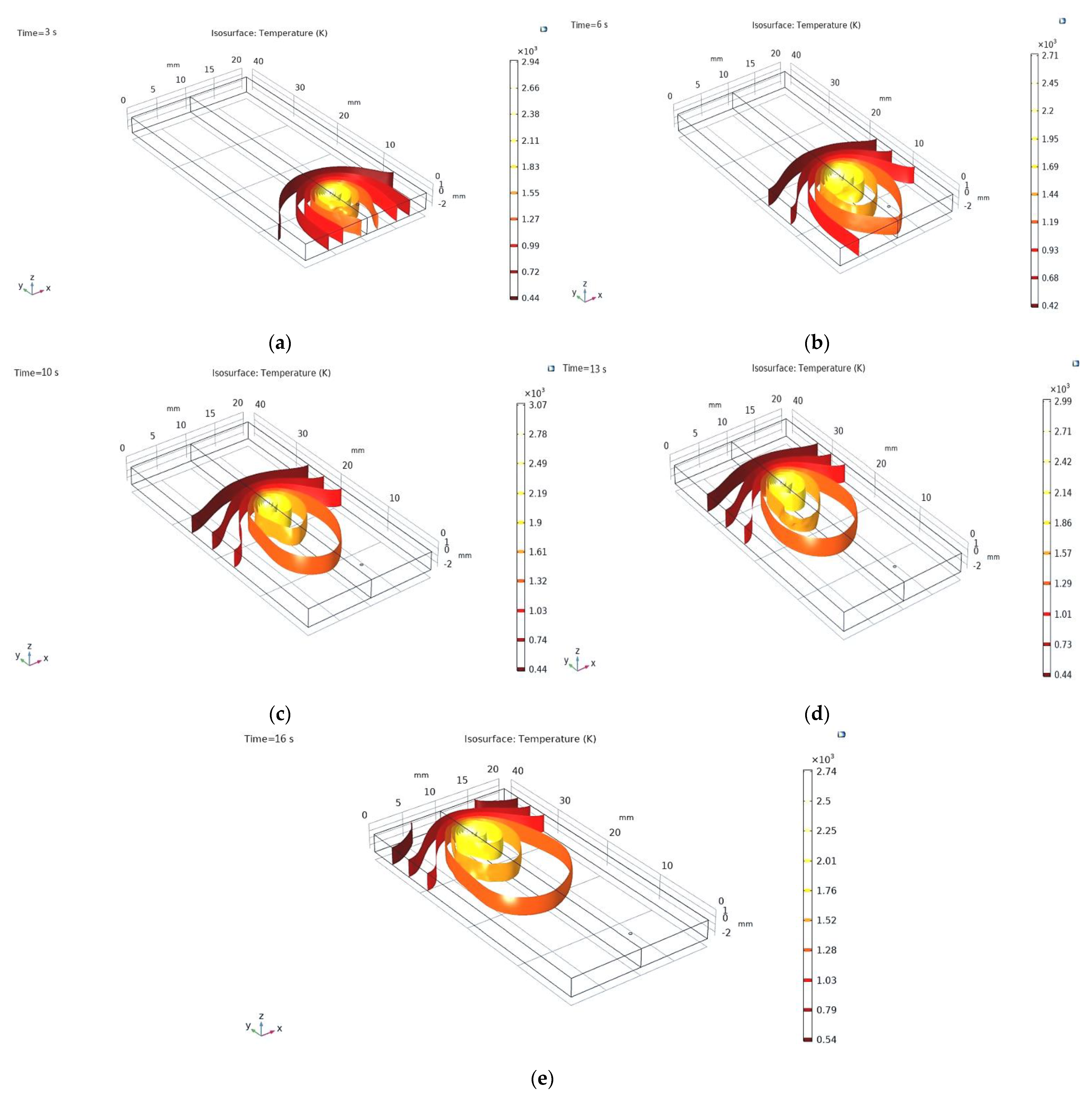
4.2. Isothermal Contours

Any time within the welding process, the welds develop at different temperatures at different positions. Isothermal contours, as shown in Figure 6, provide a view at a certain time instant in which regions or areas occupying the same temperature are within the range of 400–3000 K.

Figure 6 basically shows one of the three-dimensional representations of the transient temperature field. The isothermal elongated ellipsoid shapes form in the direction of laser source movement. The laser source is moving and focused, which results in elongated shape of the isothermal representation nearer the source. To reiterate, the transient isothermal contours show the heating and cooling phenomena and regions with metallurgical similarity that be predicted from the analysis of the contours.

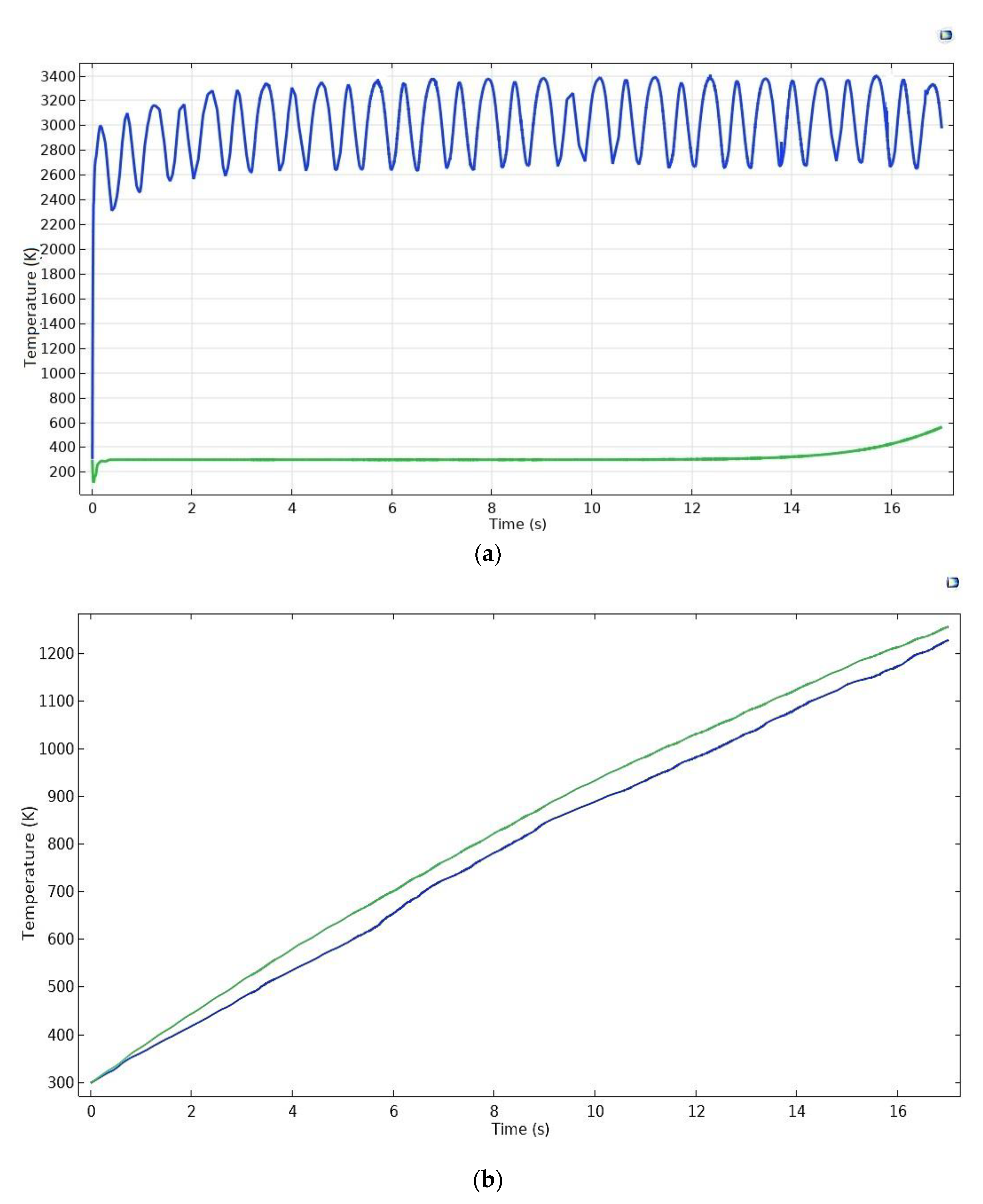
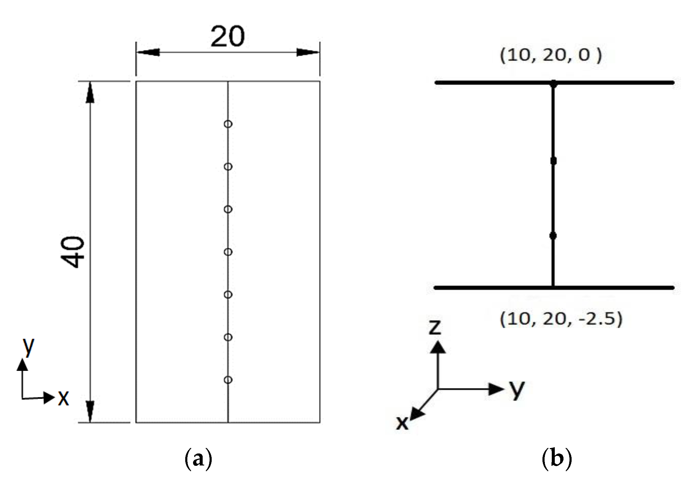
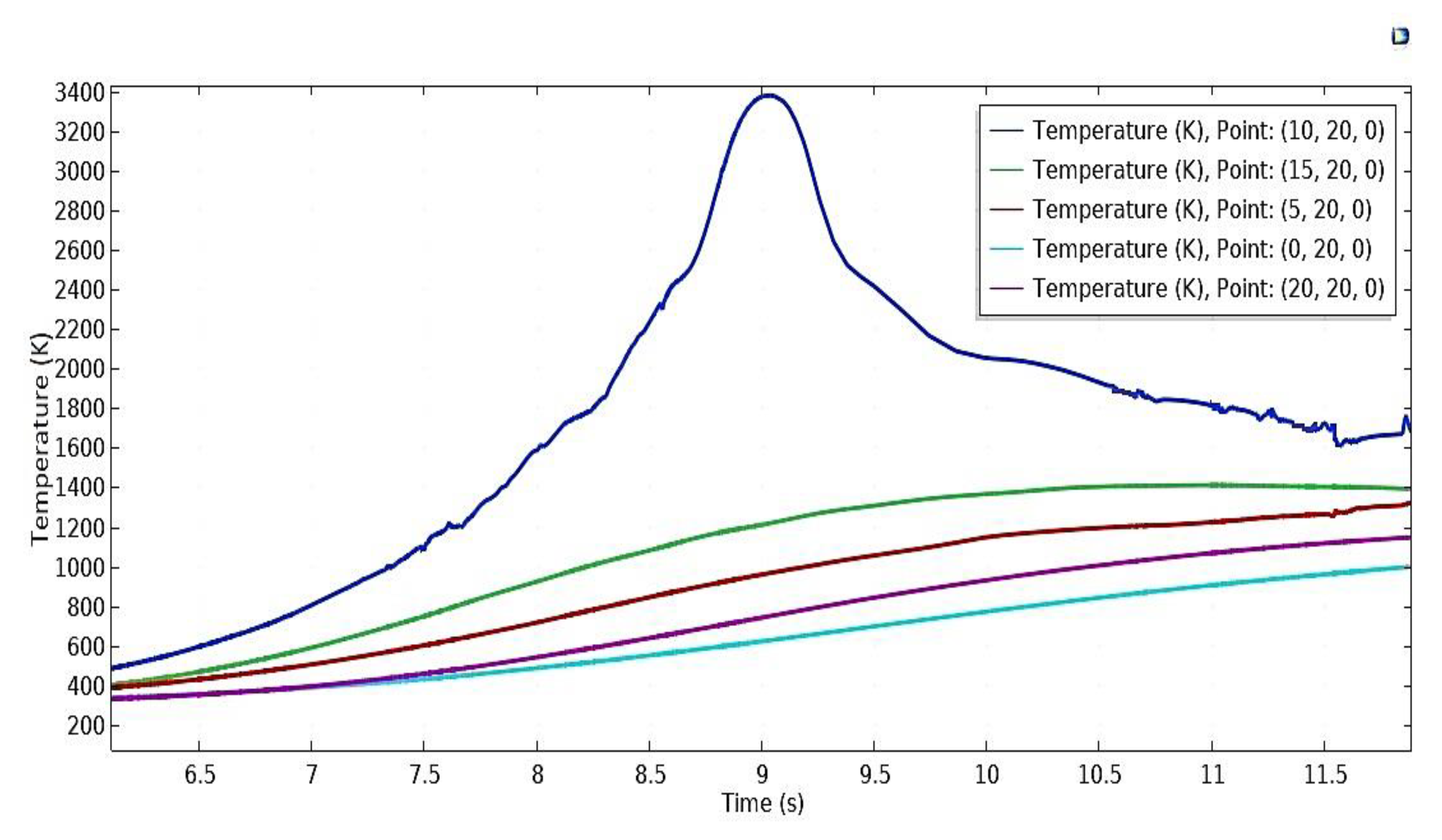
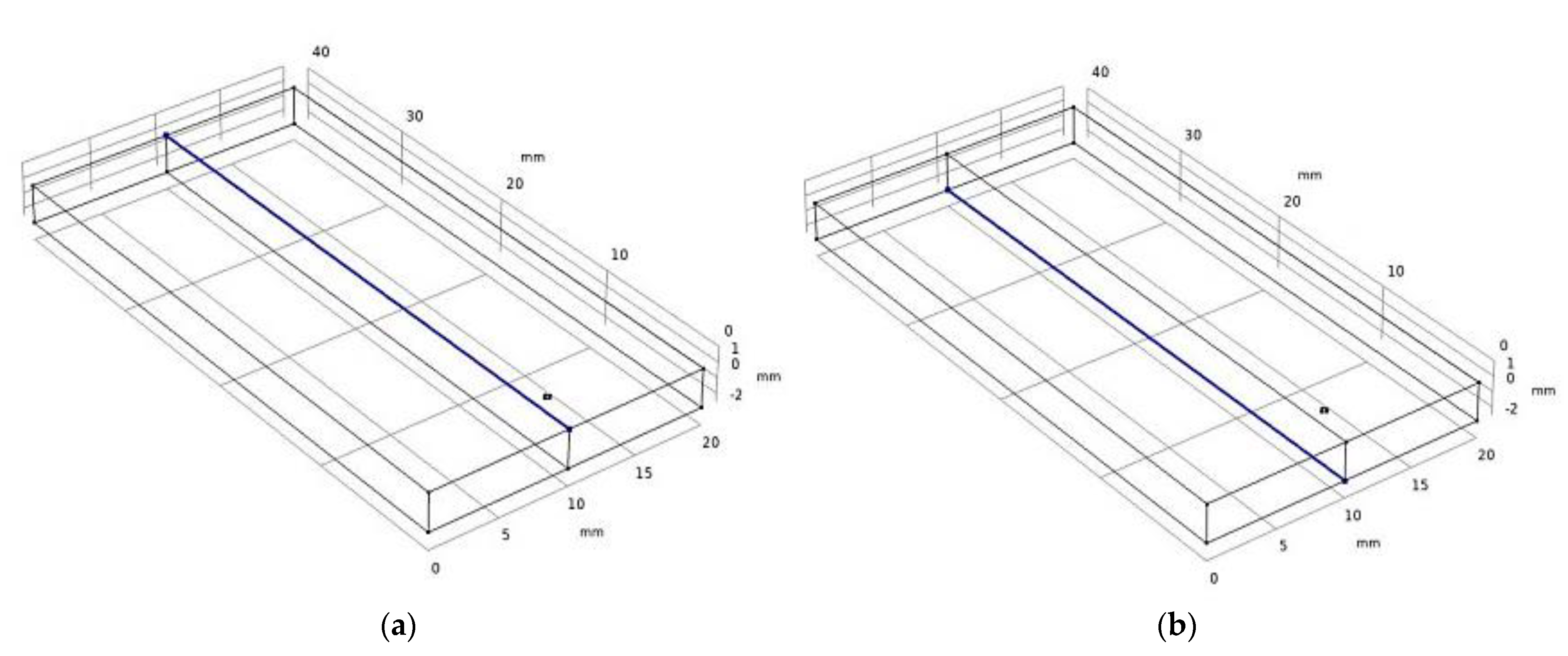
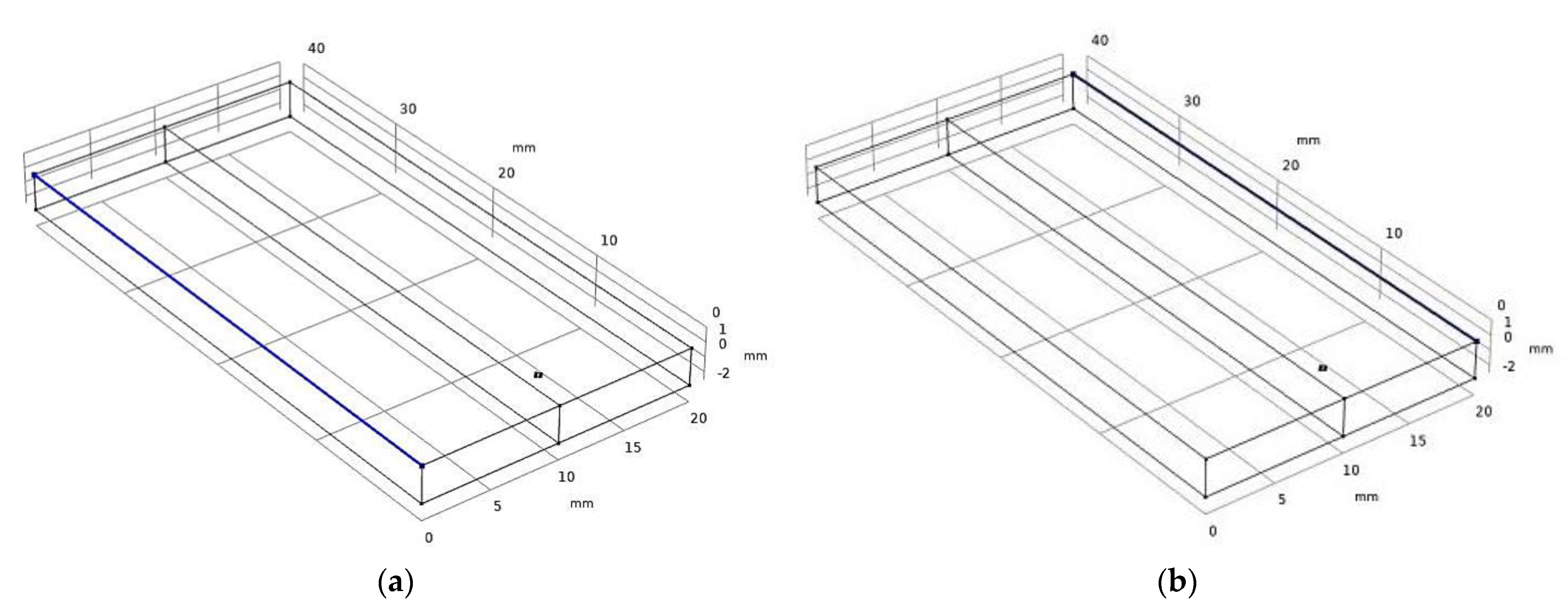
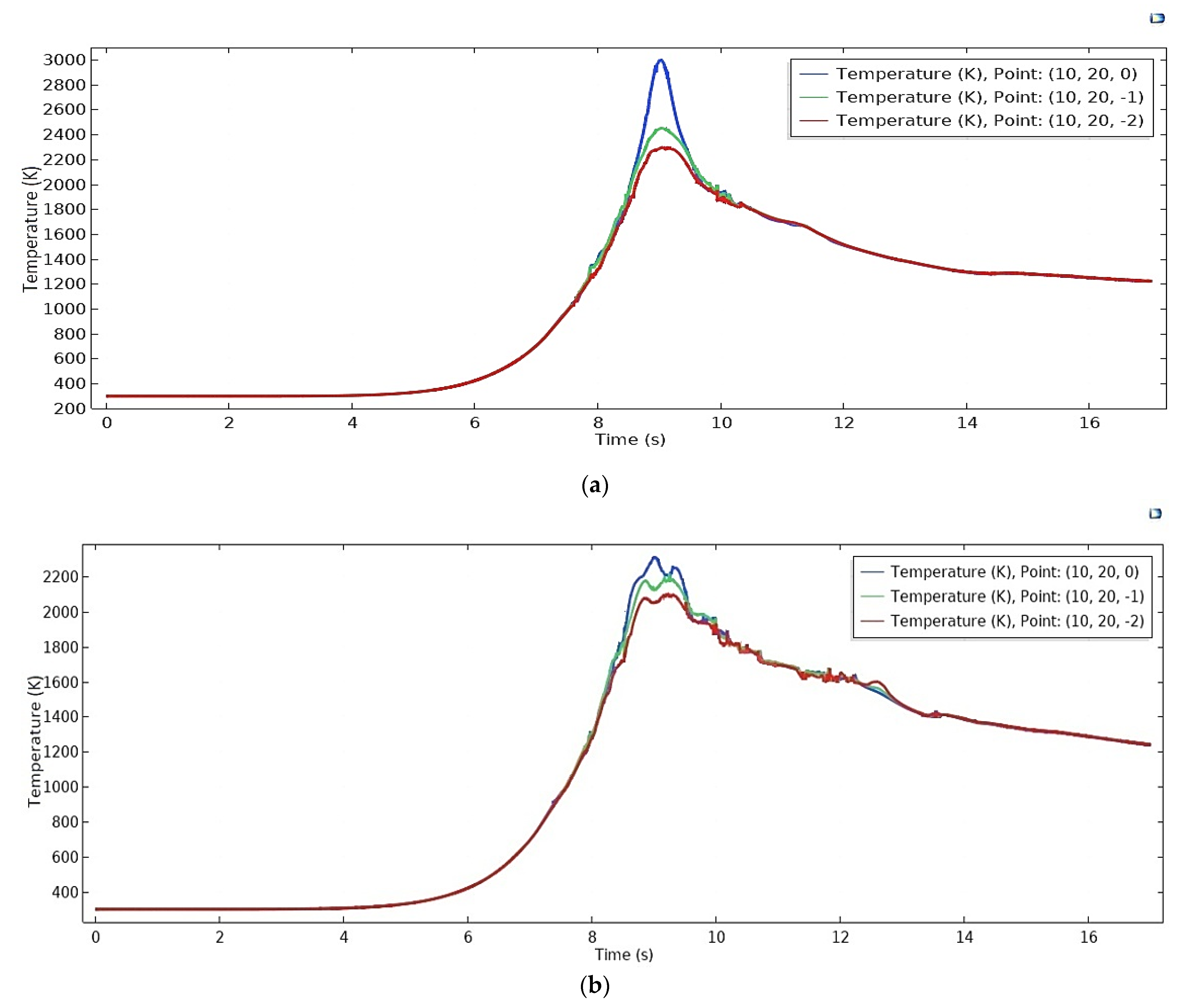
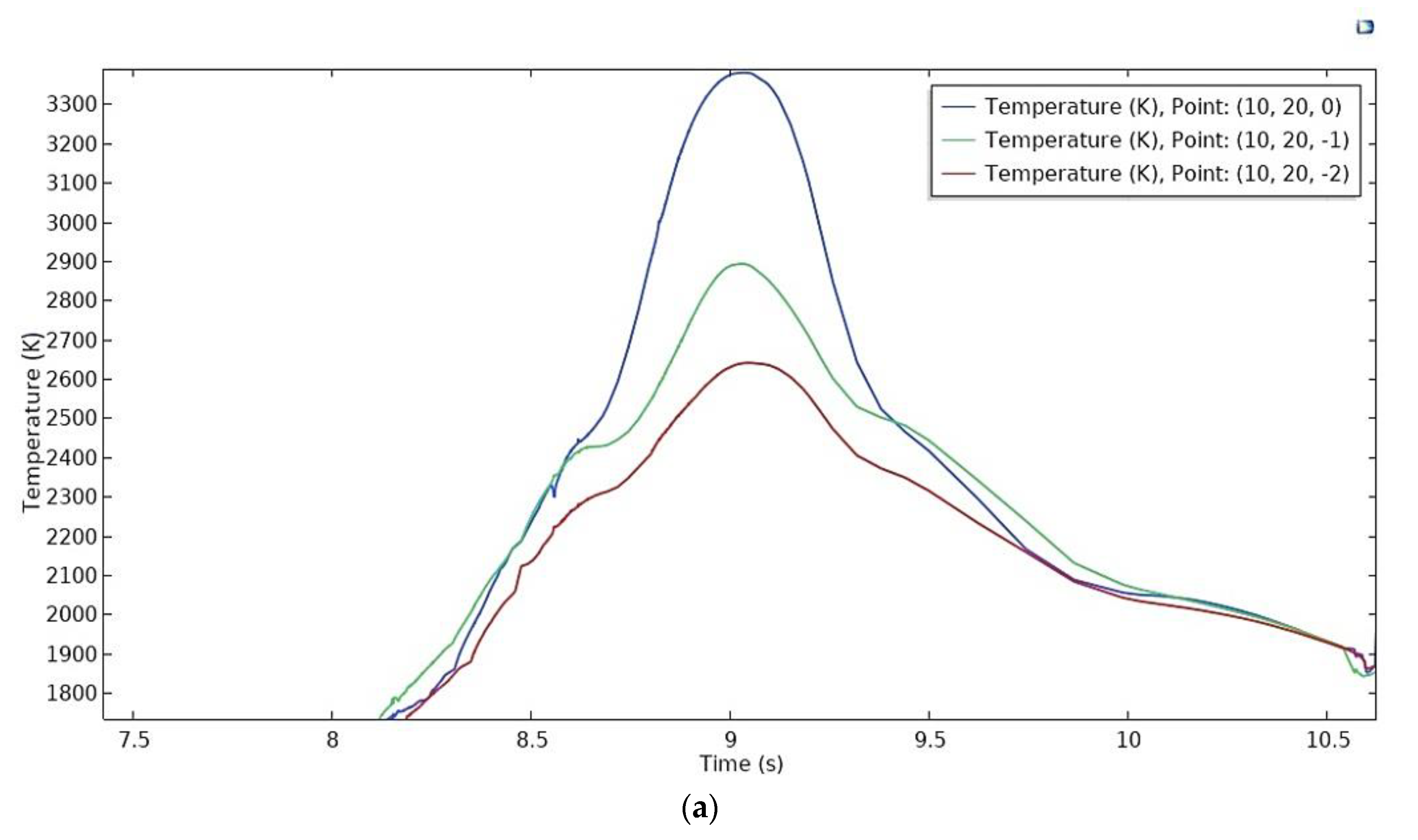
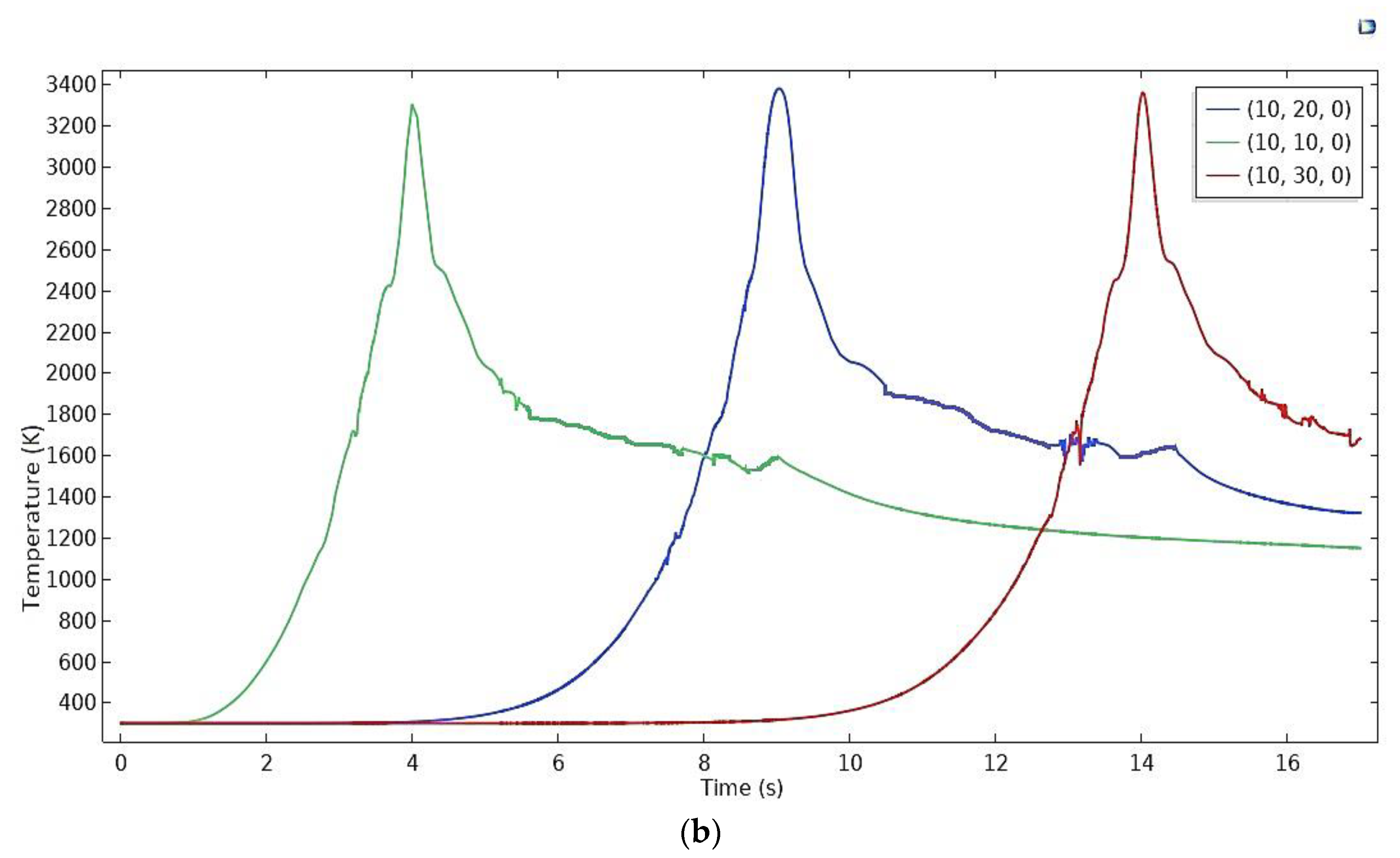
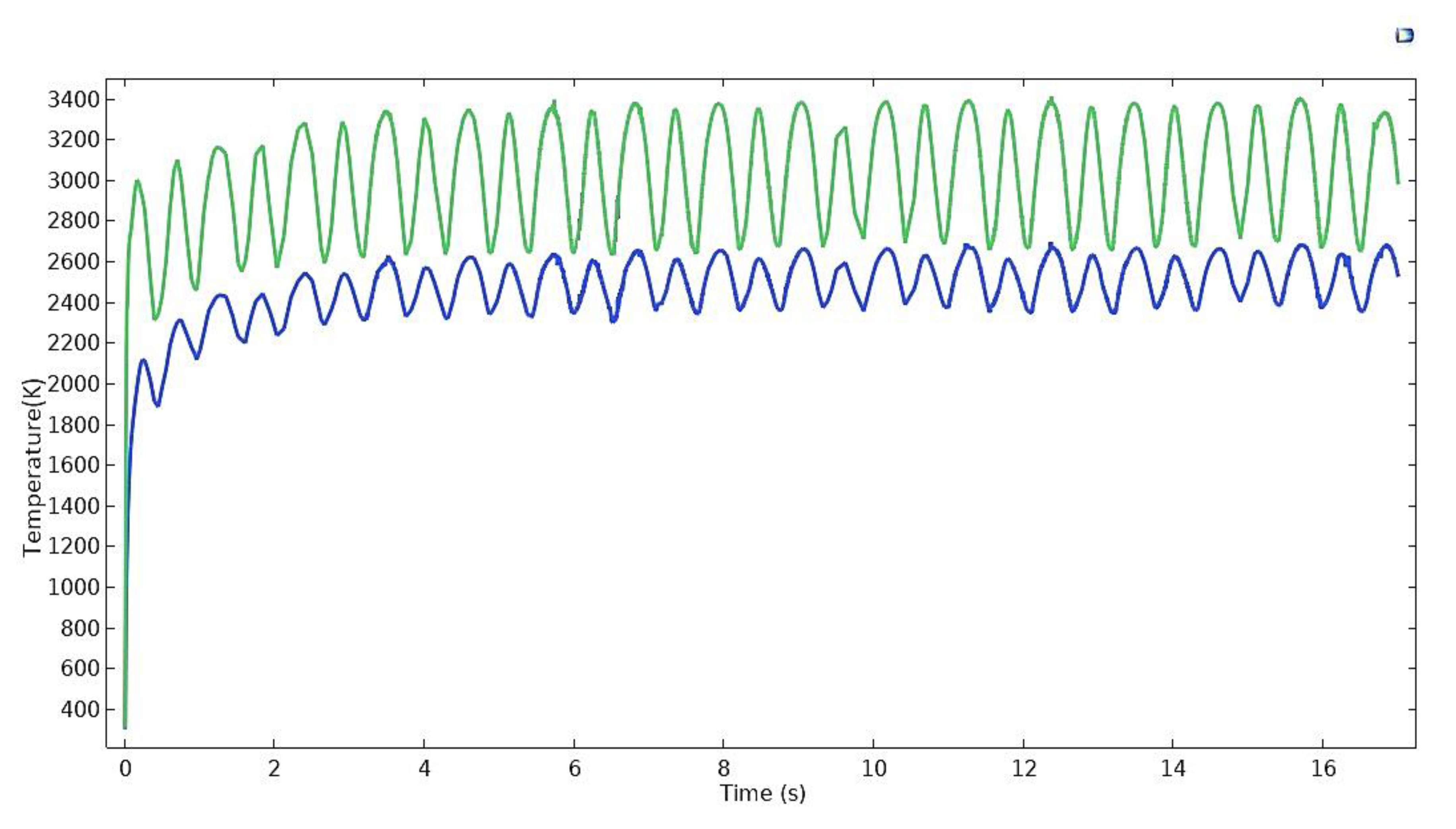
4.3. Temperature Probes

The nonlinear physical properties such as density, thermal conductivity, diffusivity, and the change in total enthalpy were simulated as functions of transient temperature distribution. Among those properties and by utilizing the model, an estimation of time-dependent temperature distribution using different probe points was highly likely. Hence, influence of temperature on the changes in microstructure and consequent changes in thermomechanical properties were highly predictable by using an iron–iron carbide diagram, time temperature transformation diagrams, etc.

The entire geometry is considered as two different temperature probe domains for two different materials. The maximum and minimum temperatures for the domains are predicted. The maximum temperature is achieved along the weld line, where the path of the laser beam is acting, as shown in Figure 7a. It reaches around 3300 K for both domains in a zero offset condition. The average temperature of the two domains is different as AISI 316 is less thermally conductive than Ti6Al4V (Figure 7b) [52]. Furthermore, the average temperature increases as the process progresses and reaches a range of 1200–1250 K after 17 s. It is a computational procedure. The temperature achieved at any point at a certain instant can be represented by a point probe on the domain, and thus the heat propagation procedure can be understood properly. There is a difference of almost 50 K in average temperature even in that short span. Nguyen et al. [53] observed a 40–50 K difference in two-domain temperatures for a dissimilar study with austenitic stainless steel and copper, due to same type of differences in thermal properties. Boundary temperature probes are taken along the weld line (see Figure 8a), perpendicular to the weld line, along with the thickness (see Figure 8b), and both sides at the same distance from the weld line. The center of the plate reaches the maximum temperature at t = 9 s, when the heat source is just at the top of the center, and started decreasing as the source moves forward due to cooling(see Figure 9b).The nature of the distribution is obvious and resembles that of a study done by placing four thermocouples 2 and 3 mm from the weld line on both sides [54]. Figure 9a shows the temperature gradient of a point together with the thickness. At a thickness of 2 mm, the temperature reaches near 2600 K. It was also observed that the peak temperature was not reached at a same time for the top and bottom surface, but there was little delay at the bottom and not the top region. This is due to the late response of absorption in the bottom surface. The bottom surface took a fraction of second more time than the top. However, both surfaces maintained maximum temperature more than the melting point. It shows that almost full penetration can be achieved as it is more than the liquidus temperature of either material. Temperature changes along the domain probes were recorded during the simulation and plotted. The boundary temperature point probe distribution on the top surface along the parallel x axis (Figure 10) is very effective for understanding the transient temperature reached at any point within the two welded parts. The peak temperature is noticed at the weld joint and it gradually decreases along the traverse direction. Peak temperatures of the two domains at the same distance began to vary as the distance increased from the weld line (Figure 11).

There is a temperature difference of up to 200 Kat points (0, 20, 0) and (20, 20, 0). The maximum temperature reached in the middle of the work pieces at traverse direction lies between 1100 K and 1200 K, while the edges along the traverse direction remain below 1000 K. This also satisfies the experimental observation of a k-type thermocouple in a welding study of two dissimilar materials [25]. Edge temperature probes along the top and bottom edge of the weld line (Figure 12) are used for temperature distribution (Figure 13). The maximum temperature reached in the z = 0 surface is more than the z = −2.5 surface, which is very normal for any inward heat flux of the welding process.

Edge probes of the two edges parallel to the weld line (x = 0 and x = 20) are considered for temperature distribution as well, as shown in Figure 14. The difference in the thermal properties of AISI 316L and Ti6Al4V makes a visible difference in the maximum temperature distributions along those edges (Figure 15). Initially, the difference is more in favor of steel for a sudden temperature increase. The difference decreases with time. The difference can be as high as 100 K and as low as 20 K.The fluctuations are reduced in radial directions because of the high resistance to heat by the parent materials. The fluctuation value comes within a range of 50–100 K for the same domain within a few millimeters, which keeps the melt zone less. The inclination of the curve is greater initially when the heat source started heating the materials. The width of the samples is 10 mm only, and from Figure 15, it is clear that the extreme edge line temperatures (parallel to the heat source) can reach up to 1200 K for both materials. This indicates that recrystallization will occur in most of the areas within the samples. For a larger width sample, the base metal area can be observed even during the heat process, but it not possible for this particular geometry. It increases flatly as the process progresses when the heating and cooling process began to occur simultaneously. Ganeriwala et al. [55] predicted the temperature from the residual stresses measured from XRD analysis. The reverse process agrees with the nature of the temperature distribution modeled here. They measured the temperature in some particular nodes and tried to explain the distribution by considering other dimensions of the material behaviors and results.

A comparison between the experiment and the simulation result generally shows the slight differences in the shape that could be due to the fact that the beam profile used in the experiments was slightly modified, which was not considered during modeling. There was a minimal difference in penetration depth and weld width between the model and simulation. The reason could be that as the temperature of the material increases there was a change in the absorptivity of the laser that was not taken into account in the model [40,41,42,43].

4.4. Offsetting the Laser Beam toward Ti-6Al-4V

It is observed from the prediction that predicted temperatures are sufficient to melt both samples. Occasionally, it is suggested for dissimilar joining to focus the laser beam on the side with the higher melting point to melting it with a higher temperature. It helps to control the IMC formation and transfer the heat toward low melting point side [2,56]. The interface faces a comparatively low temperature compared to a zero offset condition, but it should be sufficient to melt the sample with the lower melting point. In this study, it is observed that the interface can reach up to a temperature of 3200–3300 K. Offset of the laser focus by 0.3 and 0.6 mm toward Ti6Al4V side reduces the temperature of the interface points, sufficient for AISI 316L to melt. Figure 16a,b indicates that the predicted temperature of interface point (10, 20, 0) for both offset distances is sufficient to melt the steel alloy; in addition, the temperature that can be achieved in the bottom layers are also sufficient to get the penetration. The reduction in interface temperature for that particular point on the interface is comparable with that shown in Figure 9a. The noticeable reduction of the melt area in the steel side and the wider melt area in the Ti6Al4V side may cause less healthy convective flow in the molten zone around the keyhole, avoiding the formation of intermetallic phases in the weld because most heat input can be lost quickly on the Ti6Al4V side before sufficient heat is transferred into the 316L side. Ti6Al4V has a high value of thermal conductivity as well. When the laser offset is 0.35 mm toward the Ti alloy, it could be effectively connected with SS. The ratio of molten Ti alloy to SS was 95:5. A TiFe₂ layer was formed on the SS side with a width of 24 µm and the tensile strength of the joint could range up to 182 MPa [57].

5. Conclusions

A transient (time-dependent) 3D model in COMSOL is used to generate the geometry, mesh, isothermal contour, and temperature distribution along a weld line, and weld thickness is predicted for a fiber laser welding of dissimilar butt joints. Temperature-dependent materials properties, such as heat capacity, thermal conductivity, and density, are considered for both AISI 316L and Ti6Al4V. Latent heat for phase change is also accounted for in the model. The process parameters (laser power and velocity) are considered suitable for achieving full penetration of a 2.5 mm thickness butt joint of these materials. Some results are compared with offset scanning toward Ti6Al4V side as well. Major conclusions from this analysis follow:

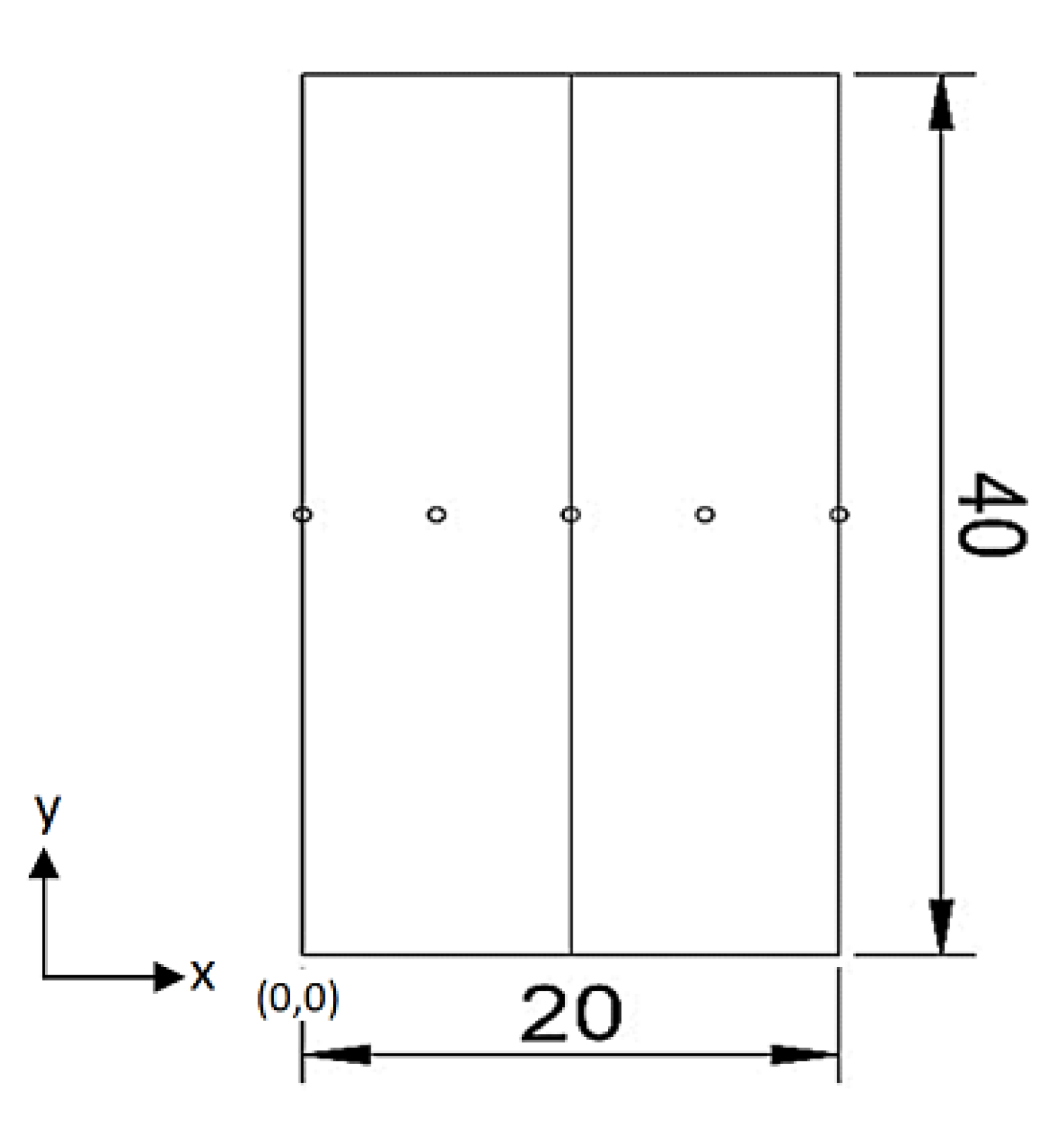
• Temperature distribution along the weld line throughout the process at laser spot irradiation shows that the average maximum temperature generated is near 3300 K. Maximum temperatures along the traverse direction (for fixed y value) on z = 0 plane in the middle (x = 5 and x = 15) and edges (x = 0 and x = 20) of the work pieces are approximately 1200 and 1000 K, respectively.
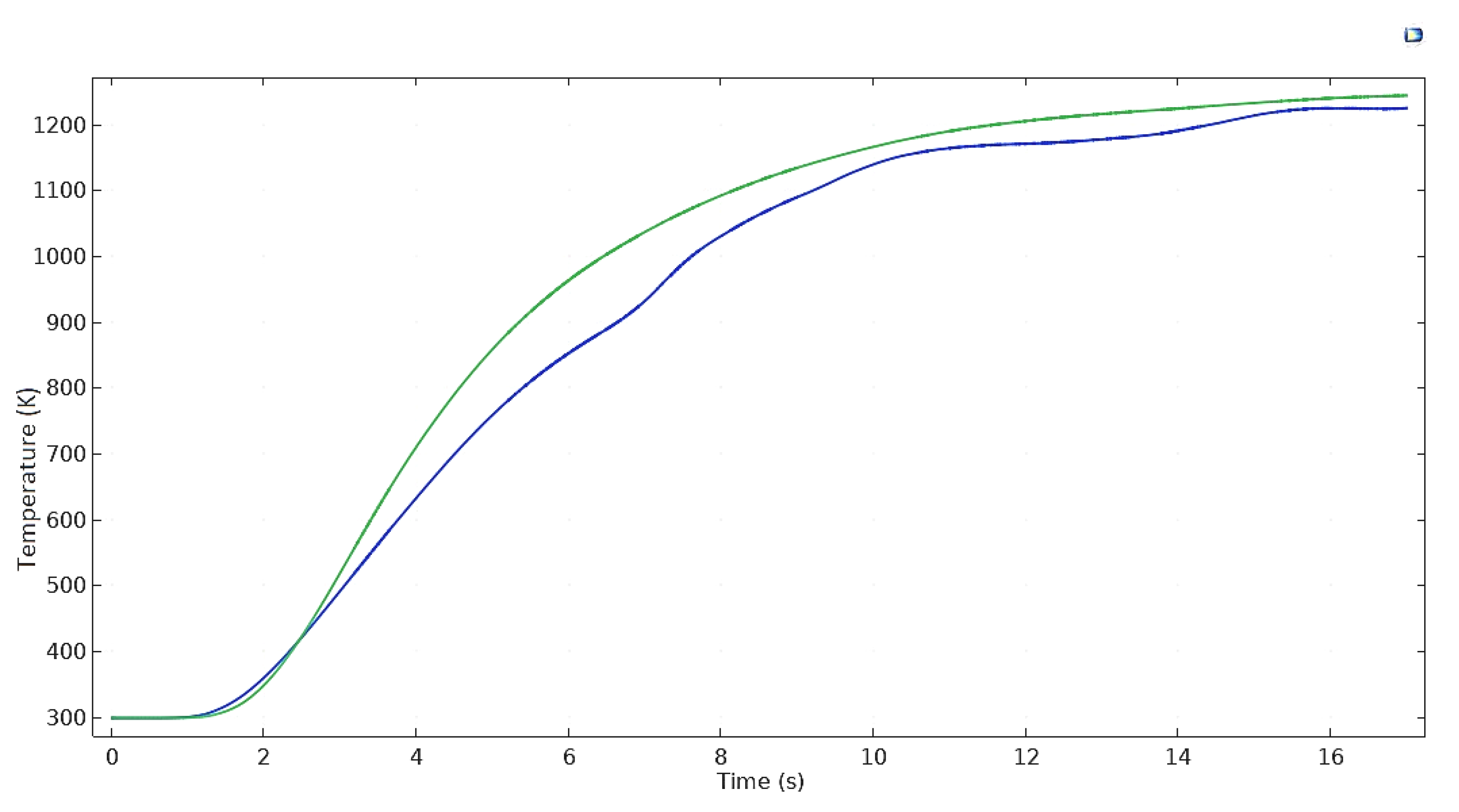
• Temperature distribution along the thickness shows that even the bottom-most surface along the z-axis achieves an average temperature near 2400 K. A significant penetration depth can be achieved. The average temperature of the two domains ranges from 1150 K to 1200 K during the process.
• There are differences in the thermal properties of these two materials. Ti6Al4V has a higher melting temperature. It would take more time than 316L to reach it, as the model was done in zero offsets. The offset of the laser heat source in the same arrangement can create a better-quality welding by adjusting the variations in thermal properties as predicted from the model. Welding interface temperature can be minimized up to 500–1000 K by offsetting the laser beam toward the Ti-6Al-4V side.
• Transient distribution of peak temperature from the weld line along the x-axis is plotted and it decreases as it moves far from the source, for obvious reason. Near the weld line, it decreases sharply and the sharpness decreases as the distance increases from the weld line. The difference of maximum temperature between the edge lines (along x = 0 and x = 20) on the z = 0 plane lies between 20 and 100 K. The maximum temperatures can reach up to 1200 K for both samples along the edges mentioned, which indicates recrystallization for AISI 316 and presence of both α phase and β phase for Ti6Al4V that occur within the sample width range.
• Transient isothermal contours help to understand the heating and cooling phenomena during the process. At higher temperature, AISI316L has a lower thermal conductivity compared to Ti6Al4V; thus, the steel part attains a higher temperature near the weld zone. Temperature history of two nearby points in traverse direction makes it understandable that even within two nearer points; one can be in heating mode and one in cooling mode. This fact demonstrates the complex type of deformation, which is the main source of residual stresses.

6. Future Scope

There is scope in the future to vary the welding speed, welding power, and offset of the heat source on either side of the weld line to predict the temperature distribution and validate it with the experimental results. It may help to optimize the parameters and realize some other parameters as well. Another area of improvement would be in a modification by increasing the mesh density of different parts while not increasing the total computational time. The results from the simulation can help identify regions that have experienced high deformation and also have high levels of temperature at different times in the welding process. This information can be used in conducting microstructural analysis to investigate any changes in the phase or find any evidence of diffusion of materials in the weld and nearby zones. Future work would include exploring the possibilities of inclusion of secondary energy sources to hasten the process of joining thick sheets of dissimilar materials.

References

1. Zhu, J.H.; Liaw, P.K.; Corum, J.M.; McCoy, H.E. High-temperature mechanical behavior of Ti-6Al-4V alloy and TiC p /Ti-6Al-4V composite. Met. Mater. Trans. A 1999, 30, 1569–1578. [Google Scholar] [CrossRef]
2. Baqer, Y.M.; Ramesh, S.; Yusof, F.; Manladan, S.M. Challenges and advances in laser welding of dissimilar light alloys: Al/Mg, Al/Ti, and Mg/Ti alloys. Int. J. Adv. Manuf. Technol. 2018, 95, 4353–4369. [Google Scholar] [CrossRef]
3. Kotadia, H.R.; Franciosa, P.; Ceglarek, D. Challenges and Opportunities in Remote Laser Welding of Steel to Aluminium. In Proceedings of the MATEC Web of Conferences; EDP Sciences: Les Ulis, France, 2019; Volume 269, p. 02012. [Google Scholar]
4. Pouranvari, M. Critical assessment 27: Dissimilar resistance spot welding of aluminium/steel: Challenges and opportunities. Mater. Sci. Technol. 2017, 33, 1705–1712. [Google Scholar] [CrossRef] [Green Version]
5. Szymlek, K. Review of Titanium and Steel Welding Methods. Adv. Mater. Sci. 2008, 8, 186–194. [Google Scholar] [CrossRef] [Green Version]
6. Emmelmann, C.; Lunding, S. Introduction to Industrial Laser Materials Processing; Rofin-Sinar Laser: Hamburg, Germany, 2000. [Google Scholar]
7. Jakubczak, K. Lasers: Applications in Science and Industry; Jakubczak, K., Ed.; BoD–Bookson Demand: Norderstedt, Germany, 2011. [Google Scholar]
8. Castillejo, M. Lasers in Materials Science; Ossi, P.M., Zhigilei, L., Eds.; Springer: Cham, Switzerland, 2014. [Google Scholar]
9. Benyounis, K.; Olabi, A.; Hashmi, M. Effect of laser welding parameters on the heat input and weld-bead profile. J. Mater. Process. Technol. 2005, 164–165, 978–985. [Google Scholar] [CrossRef] [Green Version]
10. Falvo, A.; Furgiuele, F.; Maletta, C. Laser welding of a NiTi alloy: Mechanical and shape memory behaviour. Mater. Sci. Eng. A 2005, 412, 235–240. [Google Scholar] [CrossRef]
11. Wang, P.; Chen, X.; Pan, Q.; Madigan, B.; Long, J. Laser welding dissimilar materials of aluminum to steel: An overview. Int. J. Adv. Manuf. Technol. 2016, 87, 3081–3090. [Google Scholar] [CrossRef]
12. Chen, H.-C.; Pinkerton, A.J.; Li, L. Fibre laser welding of dissimilar alloys of Ti-6Al-4V and Inconel 718 for aerospace applications. Int. J. Adv. Manuf. Technol. 2011, 52, 977–987. [Google Scholar] [CrossRef]
13. Azizpour, M.; Ghoreishi, M.; Khorram, A. Numerical simulation of laser beam welding of Ti6Al4V sheet. J. Comput. Appl. Res. Mech. Eng. 2015, 4, 145–154. [Google Scholar] [CrossRef]
14. Turňa, M.; Taraba, B.; Ambroz, P.; Sahul, M. Contribution to Numerical Simulation of Laser Welding. Phys. Procedia 2011, 12, 638–645. [Google Scholar] [CrossRef] [Green Version]
15. Kazemi, K.; Goldak, J.A. Numerical simulation of laser full penetration welding. Comput. Mater. Sci. 2009, 44, 841–849. [Google Scholar] [CrossRef]
16. Tsirkas, S.; Papanikos, P.; Kermanidis, T. Numerical simulation of the laser welding process in butt-joint specimens. J. Mater. Process. Technol. 2003, 134, 59–69. [Google Scholar] [CrossRef]
17. Guoming, H.; Jian, Z.; JianQang, L. Dynamic simulation of the temperature field of stainless steel laser welding. Mater. Des. 2007, 28, 240–245. [Google Scholar] [CrossRef]
18. Mohanty, S.; Laldas, C.K.; Roy, G.G. A New Model for Keyhole Mode Laser Welding Using FLUENT. Trans. Indian Inst. Met. 2012, 65, 459–466. [Google Scholar] [CrossRef]
19. Attarha, M.; Sattari-Far, I. Study on welding temperature distribution in thin welded plates through experimental measurements and finite element simulation. J. Mater. Process. Technol. 2011, 211, 688–694. [Google Scholar] [CrossRef]
20. Shanmugam, N.S.; Buvanashekaran, G.; Sankaranarayanasamy, K.; Kumar, S.R. A transient finite element simulation of the temperature and bead profiles of T-joint laser welds. Mater. Des. 2010, 31, 4528–4542. [Google Scholar] [CrossRef]
21. Multiphysics COMSOL. Introduction to COMSOL Multiphysics®; COMSOL Multiphysics: Burlington, MA, USA, 2018. [Google Scholar]
22. Dickinson, E.; Ekström, H.; Fontes, E. COMSOL Multiphysics®: Finite element software for electrochemical analysis. A mini-review. Electrochem. Commun. 2014, 40, 71–74. [Google Scholar] [CrossRef]
23. Ranjbarnodeh, E.; Serajzadeh, S.; Kokabi, A.H.; Fischer, A. Prediction of temperature distribution in dissimilar arc welding of stainless steel to carbon steel. Proc. Inst. Mech. Eng. Part B J. Eng. Manuf. 2012, 226, 117–125. [Google Scholar] [CrossRef]
24. Akbari, M.; Saedodin, S.; Toghraie, D.; Shoja-Razavi, R.; Kowsari, F. Experimental and numerical investigation of temperature distribution and melt pool geometry during pulsed laser welding of Ti6Al4V alloy. Opt. Laser Technol. 2014, 59, 52–59. [Google Scholar] [CrossRef]
25. Kumar, P.; Sinha, A.N. Studies of temperature distribution for laser welding of dissimilar thin sheets through finite element method. J. Braz. Soc. Mech. Sci. Eng. 2018, 40, 455. [Google Scholar] [CrossRef]
26. Attar, M.A.; Ghoreishi, M.; Beiranvand, Z.M. Prediction of weld geometry, temperature contour and strain distribution in disk laser welding of dissimilar joining between copper & 304 stainless steel. Optik 2020, 219, 165288. [Google Scholar] [CrossRef]
27. Li, Z.; Rostam, K.; Panjehpour, A.; Akbari, M.; Karimipour, A.; Rostami, S. Experimental and numerical study of temperature field and molten pool dimensions in dissimilar thickness laser welding of Ti6Al4V alloy. J. Manuf. Process. 2020, 49, 438–446. [Google Scholar] [CrossRef]
28. Ai, Y.; Jiang, P.; Wang, C.; Mi, G.; Geng, S. Experimental and numerical analysis of molten pool and keyhole profile during high-power deep-penetration laser welding. Int. J. Heat Mass Transf. 2018, 126, 779–789. [Google Scholar] [CrossRef]
29. Akbari, M.; Saedodin, S.; Panjehpour, A.; Hassani, M.; Afrand, M.; Torkamany, M.J. Numerical simulation and designing artificial neural network for estimating melt pool geometry and temperature distribution in laser welding of Ti6Al4V alloy. Optik 2016, 127, 11161–11172. [Google Scholar] [CrossRef]
30. Fey, A.; Ulrich, S.; Jahn, S.; Schaaf, P. Numerical analysis of temperature distribution during laser deep welding of duplex stainless steel using a two-beam method. Weld. World 2020, 64, 623–632. [Google Scholar] [CrossRef]
31. Kumar, K.S. Analytical Modeling of Temperature Distribution, Peak Temperature, Cooling Rate and Thermal Cycles in a Solid Work Piece Welded by Laser Welding Process. Procedia Mater. Sci. 2014, 6, 821–834. [Google Scholar] [CrossRef] [Green Version]
32. Tsirkas, S. Numerical simulation of the laser welding process for the prediction of temperature distribution on welded aluminium aircraft components. Opt. Laser Technol. 2018, 100, 45–56. [Google Scholar] [CrossRef]
33. Shah, A.; Kumar, A.; Ramkumar, J. Analysis of transient thermo-fluidic behavior of melt pool during spot laser welding of 304 stainless-steel. J. Mater. Process. Technol. 2018, 256, 109–120. [Google Scholar] [CrossRef]
34. Wang, R.; Lei, Y.; Shi, Y. Numerical simulation of transient temperature field during laser keyhole welding of 304 stainless steel sheet. Opt. Laser Technol. 2011, 43, 870–873. [Google Scholar] [CrossRef]
35. Lee, K.-H.; Yun, G.J. A novel heat source model for analysis of melt Pool evolution in selective laser melting process. Addit. Manuf. 2020, 36, 101497. [Google Scholar] [CrossRef]
36. Steen, W.M.; Dowden, J.; Davis, M.; Kapadia, P. A point and line source model of laser keyhole welding. J. Phys. D Appl. Phys. 1988, 21, 1255–1260. [Google Scholar] [CrossRef]
37. Tseng, W.; Aoh, J. Simulation study on laser cladding on preplaced powder layer with a tailored laser heat source. Opt. Laser Technol. 2013, 48, 141–152. [Google Scholar] [CrossRef]
38. Xu, G.X.; Wu, C.S.; Qin, G.L.; Wang, X.Y.; Lin, S.Y. Adaptive volumetric heat source models for laser beam and laser + pulsed GMAW hybrid welding processes. Int. J. Adv. Manuf. Technol. 2011, 57, 245–255. [Google Scholar] [CrossRef]
39. Jayanthi, A.; Venkatramanan, K.; Kumar, K. Modeling and simulation for welding of AISI316l stainless steels using Pulsed Nd:YAG Laser. Int. J. Mater. Sci. 2017, 12, 39–50. [Google Scholar]
40. Indhu, R.; Tak, M.; Vijayaraghavan, L.; Soundarapandian, S. Microstructural evolution and its effect on joint strength during laser welding of dual phase steel to aluminium alloy. J. Manuf. Process. 2020, 58, 236–248. [Google Scholar] [CrossRef]
41. Indhu, R.; Divya, S.; Tak, M.; Soundarapandian, S. Microstructure development in Pulsed Laser Welding of Dual Phase Steel to Aluminium Alloy. Procedia Manuf. 2018, 26, 495–502. [Google Scholar] [CrossRef]
42. Indhu, R.; Soundarapandian, S.; Vijayaraghavan, L. Yb: YAG laser welding of dual phase steel to aluminium alloy. J. Mater. Process. Technol. 2018, 262, 411–421. [Google Scholar] [CrossRef]
43. Indhu, R.; Tak, M.; Vijayaraghavan, L.; Soundarapandian, S. Microstructural and mechanical properties of complex phase steel to aluminium alloy welded dissimilar joint. Procedia Manuf. 2020, 48, 267–272. [Google Scholar] [CrossRef]
44. Paschotta, R. Encyclopedia of Laser Physics and Technology; Wiley-Vch: Berlin, Germany, 2008; Volume 1. [Google Scholar]
45. Noy, A. (Ed.) Handbook of Molecular Force Spectroscopy; Springer Science & Business Media: Heidelberg, Germany, 2007. [Google Scholar]
46. Lakoba, T.I.; Kaup, D.J. Hermite-Gaussian expansion for pulse propagation in strongly dispersion managed fibers. Phys. Rev. 1998, 58, 6728–6741. [Google Scholar] [CrossRef]
47. Balasubramanian, K.R.; Shanmugam, N.S.; Buvanashekaran, G.; Sankaranarayanasamy, K. Numerical and experimental investigation of laser beam welding of AISI304 stainless steel sheet. Adv. Prod. Eng. Manag. 2008, 3, 93–105. [Google Scholar]
48. Shanmugam, N.S.; Buvanashekaran, G.; Sankaranarayanasamy, K. Experimental investigation and finite element simulation oflaser beam welding of AISI304 stainless steel sheet. Exp. Tech. 2010, 34, 25–36. [Google Scholar] [CrossRef]
49. Boivineau, M.; Cagran, C.; Doytier, D.; Eyraud, V.; Nadal, M.-H.; Wilthan, B.; Pottlacher, G. Thermophysical Properties of Solid and Liquid Ti-6Al-4V (TA6V) Alloy. Int. J. Thermophys. 2006, 27, 507–529. [Google Scholar] [CrossRef]
50. Kim, C.S. Thermophysical Properties of Stainless Steels; (No.ANL-75-55); Argonne National Lab.: Lemont, IL, USA, 1975.
51. Xiong, L.; Mi, G.; Wang, C.; Zhu, G.; Xu, X.; Jiang, P. Numerical Simulation of Residual Stress for LaserWelding of Ti-6Al-4VAlloy Considering Solid-State Phase Transformation. J. Mater. Eng. Perform. 2019, 28, 3349–3360. [Google Scholar] [CrossRef]
52. Mertens, A.; Reginster, S.; Paydas, H.; Contrepois, Q.; Dormal, T.; Lemaire, O.; Lecomte-Beckers, J. Mechanical properties of alloy Ti–6Al–4V and of stainless steel 316L processed by selective laser melting: Influence of out-of-equilibrium microstructures. Powder Met. 2014, 57, 184–189. [Google Scholar] [CrossRef]
53. Nguyen, Q.; Azadkhou, A.; Akbari, M.; Panjehpour, A.; Karimipour, A. Experimental investigation of temperature field and fusion zone microstructure in dissimilar pulsed laser welding of austenitic stainless steel and copper. J. Manuf. Process. 2020, 56, 206–215. [Google Scholar] [CrossRef]
54. Casalino, G.; Mortello, M. Modeling and experimental analysis of fiber laser offset welding of Al-Ti butt joints. Int. J. Adv. Manuf. Technol. 2015, 83, 89–98. [Google Scholar] [CrossRef]
55. Ganeriwala, R.; Strantza, M.; King, W.; Clausen, B.; Phan, T.; Levine, L.; Brown, D.; Hodge, N. Evaluation of a thermomechanical model for prediction of residual stress during laser powder bed fusion of Ti-6Al-4V. Addit. Manuf. 2019, 27, 489–502. [Google Scholar] [CrossRef]
56. Casalino, G.; Mortello, M.; Peyre, P. FEM Analysis of Fiber Laser Welding of Titanium and Aluminum. Procedia CIRP 2016, 41, 992–997. [Google Scholar] [CrossRef] [Green Version]
57. Zhang, Y.; Zhou, J.; Sun, D.; Gu, X. Nd:YAG laser welding of dissimilar metals of titanium alloy to stainless steel without filler metal based on a hybrid connection mechanism. J. Mater. Res. Technol. 2020, 9, 1662–1672. [Google Scholar] [CrossRef]
Figure 1. Geometry of the model.
Applsci 11 05829 g001
Figure 2. Profile of Hermit–Gaussian heat source function.
Applsci 11 05829 g002
Figure 3. Temperature-dependent property plots for AISI 316L (ac) and Ti-6Al-4V (df).
Applsci 11 05829 g003
Figure 4. Mesh modeling of the weld joint assembly.
Applsci 11 05829 g004
Figure 5. Temperature propagation contours at (a) t = 3 s, (b) t = 6 s, (c) t = 10 s, (d) t =13 s, and (e) t =16 s.
Applsci 11 05829 g005
Figure 6. Isothermal contours at (a) t = 3 s, (b) t = 6 s, (c) t = 10 s, (d) t = 13 s, and (e) t = 16 s.
Applsci 11 05829 g006
Figure 7. (a) Maximum and minimum temperature computational plot for domain 1 (AISI 316L side) and (b) comparative average temperature with time for domain 1 (green) and domain 2 (blue).
Applsci 11 05829 g007
Figure 8. Boundary temperature probe points (a) along weld line (y axis) and (b) along the thickness (z axis).
Applsci 11 05829 g008
Figure 9. Temperature distribution of three different points (a) along the thickness perpendicular to the weld line and (b) along the weld line.
Applsci 11 05829 g009aApplsci 11 05829 g009b
Figure 10. Boundary temperature probe points perpendicular to weld line (x-axis).
Applsci 11 05829 g010
Figure 11. Temperature distribution of temperature probes of two different domains having the same Y = 20 mm.
Applsci 11 05829 g011
Figure 12. Edge temperature probe along the direction of welding: (a) z = 0 and (b) z = –2.5.
Applsci 11 05829 g012
Figure 13. Maximum temperature (computational) on the edge temperature probes along weld line at Z = 0 (green) and Z = −2.5 (blue).
Applsci 11 05829 g013
Figure 14. Edge temperature probes (a) x = 0, (b) x = 20, and on the z = 0 surface.
Applsci 11 05829 g014
Figure 15. Maximum temperature (transient) of edge probes x = 0 mm (green) and x = 20 mm (blue).
Applsci 11 05829 g015
Figure 16. Temperature distribution of three different points on interface: (a) 0.3 mm offset and (b) 0.6 mm offset toward Ti6Al4V.
Applsci 11 05829 g016