Abstract
The transfer function method is a common method for establishing a traveling wave field in a sound tube to measure the reflection and transmission coefficient of underwater material. The voltage applied to the secondary sound source can be calculated in accordance with the transfer matrix between the sound sources and hydrophones, then a traveling wave field can be established in the sound tube. However, the transfer function must be remeasured when the measurement frequency needs to be changed. A checking procedure of the traveling wave field in the sound tube is essential before measuring underwater acoustic material. If it is not an accurate traveling wave field, the secondary sound source signal should be corrected until the traveling wave field meets the requirements. To address these problems, an adaptive control method for generating plane traveling waves is proposed. The phase difference of sound pressures measured using the two hydrophones between the secondary sound source and the sample is used as the objective function in the adaptive algorithm, and the amplitude and phase of the secondary sound source can be obtained using the adaptive control system in the frequency domain. When a traveling wave field is formed, the reflection and transmission coefficient of the sample can be measured at the same time. With this method, the procedure of testing the traveling wave field is omitted. If the state of the primary sound source changes, the signal form of the secondary sound source can be changed immediately. Therefore, the efficiency of material measurement is improved. Theoretically, this method can obtain the most matching signal form of the secondary sound source, such that the accuracy of this method is remarkably high. Simulation and experimental results in this paper show that the measurement accuracy is reliable within the frequency range of 100–2500 Hz.
1. Introduction
The performance parameters of underwater material, such as the anti-acoustic baffle and anechoic tile, are significant, and the measurement parameters that reflecting its acoustic performance are the reflection and transmission coefficient of the sample under the plane wave perpendicular to the incident. Therefore, accurate measurement of the complex reflection and transmission coefficient of underwater materials is particularly important in the field of underwater acoustic engineering [1,2]. With the development of marine technology, the working frequency of underwater acoustic materials gradually extends to a low frequency. In the early stage of material design, the acoustic performance of a material is mainly evaluated using the test results of small samples in an acoustic tube [3,4,5,6,7,8,9,10,11]. The basic principle of the acoustic tube measurement is to generate plane waves below the first-order cut-off frequency in the acoustic tube by controlling the sound source at one end of the acoustic tube [12]. The acoustic tube method, also known as the impedance tube method, can be divided into standing wave tube method [13,14,15,16,17,18], pulse tube method [19,20,21,22,23], and traveling wave tube (TWT) method from the perspective of the sound field formed in the tube.
Among them, the pulse tube method is suitable for high frequency. As the test frequency decreases, the required length of the acoustic tube increases. Thus, the reflection and transmission coefficient of materials are difficult to test in a low frequency. When the acoustic properties of materials are tested in a standing wave tube, only the acoustic reflection coefficient can be obtained, and the acoustic impedance value of the sound tube’s downstream is necessary to obtain [24,25,26,27,28,29,30,31]. If the TWT method is used to measure the reflection and transmission coefficient of materials, the sample is placed in the middle of the acoustic tube, the main sound source is installed upstream of the acoustic tube, and the secondary sound source is installed downstream of the acoustic tube to absorb transmission–reflection sound waves. Continuous plane traveling waves are generated using the main sound source. In an ideal case, the traveling wave field can be formed in the half part of the acoustic tube under the material, that is, the length of the acoustic tube can be regarded as infinite. Therefore, the TWT method can be used to obtain the low-frequency acoustic reflection and transmission coefficients of materials at the same time.
The control methods for TWT include passive and active control [32,33,34,35,36,37]. The principle of passive control is adding a sound-absorbing material downstream of the acoustic tube to ensure that the transmission–reflection sound waves are absorbed. However, reflected sound will exist in the right part of the tube because the sound absorption performance of the sound-absorbing material decreases with the decrease in frequency. If the active control method is adopted, the relationship between the secondary sound source and its surface reflection coefficient shall be established first [38], then the secondary sound source loading signal shall be controlled in accordance with the change in the reflection coefficient to change its surface reflection coefficient. When the reflection coefficient reduces to a certain value, a traveling wave field can be generated. Although this method can accurately establish a traveling wave field in a sound tube, some shortcomings, such as the complex calculation and the cumbersome control process, are not inevitable. The establishment of a traveling wave field will also require considerable time. Consequently, this method has gradually been abandoned.
Currently, the transfer function method is immensely popular. This method can obtain the desired voltage value, which will be applied to the secondary sound source by calculating the matrix between two sound sources and hydrophones. Then, the establishment of a wave field in a sound tube is completed. Lastly, the reflection and transmission coefficients of the material to be tested will be obtained. The transfer function method can rapidly determine the desired voltage value of the secondary sound source. Nevertheless, when the measurement frequency changes, the transfer matrix between the sound sources and hydrophones should be remeasured, which increases the workload of researchers.
In this paper, a control method for TWT based on the adaptation principle is proposed to form a traveling wave field in underwater acoustic tube quickly and accurately, so as to improve the measurement accuracy and efficiency of the material acoustic reflection coefficient and transmission coefficient. The traveling wave relationship can be satisfied by adjusting the amplitude and phase of an acoustic signal in any two positions of TWT. This method can automatically establish a traveling wave field and calculate the reflection and transmission coefficients of materials when frequency changes. Lastly, the reliability of the TWT adaptive control principle is verified through simulation and experiment.
2. Background
2.1. Reflection and Transmission Coefficients
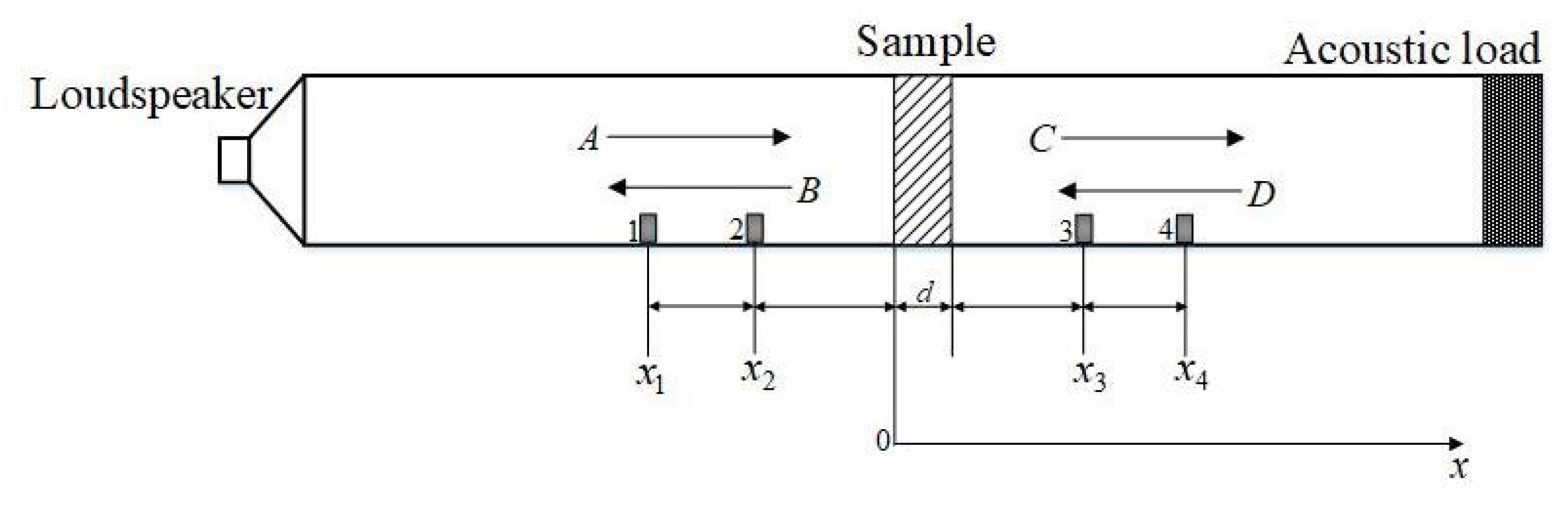
The four-hydrophone measurement method is frequently used to measure reflection and transmission coefficients [39]. The measuring impedance tube model is shown in Figure 1. The impedance tube is designed to obtain the acoustic information of the upstream and downstream sections in this tube by using four microphones. Such information can be used to calculate the reflection and transmission coefficients in accordance with corresponding formulas.

Figure 1.
Four hydrophone measurement model.
A primary sound source in the upstream section excites incidence waves, transmits them to the downstream section after passing the test sample, and meets the boundary condition in the form of acoustic load. Incidence and reflected waves are formed on the left (A and B) and right (C and D) hands of the test sample, respectively. The sound pressure of both sides of the sample can be expressed as:
where d is the thickness of the test sample; j is the imaginary unit; and represents the wave-number, which can be obtained using the formula , where is the angular frequency and is the sound velocity. The amplitudes of the hydrophones at four positions (, and ) are known, and the incidence wave (A), reflection wave (B), transmission–incidence wave (C), and transmission-reflection wave (D) can be shown as:
The transmission–reflection wave (D) will be removed if the end of the impedance tube is an anechoic termination. In that condition, the complex reflection coefficient (R) and transmission coefficient (T) of the test sample can be obtained as follows:
2.2. Transfer Function Method for Active Control Termination
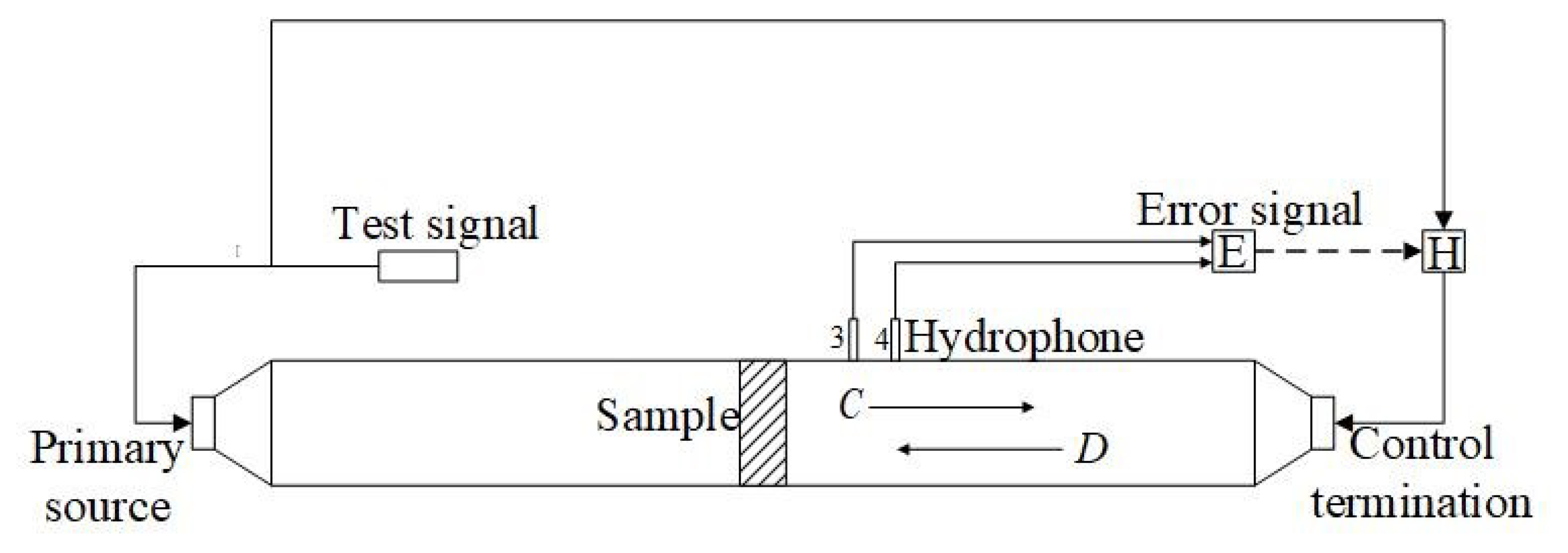
In the past, researchers eliminated the transmission–reflection wave through placing absorption materials at the end of an impedance tube. However, the transmission–reflection wave is difficult to cancel completely, especially in a low-frequency range. Thus, researchers began trying to solve this problem with the active control method. For instance, Tzili and Bustamante designed a measurement system with active absorption termination downstream of an impedance tube, and the simplified system model is shown in Figure 2 [40].
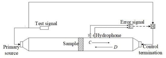
Figure 2.
Transfer function method measurement model.
They regarded the relationship between and as an error signal and determined the transfer function between the error signal and input of active control termination. The transmission–reflection wave D will be cancelled by the corresponding sound wave excited by active control termination.
The aim of this system is eliminating the transmission-reflection wave D with active control termination by minimizing the error signal. Initially, they determined the transfer function between the error signal and the sound pressure amplitude of D. The sound pressure of hydrophones at locations 3 and 4 can be written as follows:
From Equations (9) and (10),
The error signal extracted from Equation (11) is as follows:
Assuming that represents the transfer function between primary source and error signal and is the transfer function between control termination and signal error, the error signal in the form of frequency domain is expressed as follows:
where is the transfer function between error signal and active control termination that should be measured, and is the form of frequency domain of the test signal. Then, the quadratic error is minimized to zero to obtain the transfer function , as shown as follows:
where (*) indicates the complex conjugate, and is the regularization level [41]. In this way, the reflected sound wave D can be absorbed by active termination in the downstream section of the tube. In this condition, the reflection coefficient R and transmission coefficient T can be obtained using Equations (7) and (8).
3. Adaptive Control Method
Although active control termination with the transfer function method is applied to the measurement acoustic parameters of sample, some defects are unavoidable for this method. The accuracy degree of the measurement result is mainly affected by two factors: the consistency between hydrophones and the accuracy degree of the transfer function measured between primary source and error signal and between secondary source and error signal. In addition, researchers need to measure the transfer function again once the test frequency changes, which causes the process of measuring sample properties to be overly complex. In this study, we adopt an adaptive algorithm (least mean squares, LMS) to control active termination, which can adjust in time the output of the secondary source automatically in accordance with the error signal. In this way, researchers do not need to measure the transfer function, such that we do not need to consider the measurement error caused by an inaccurate transfer function. The operation process is simplified greatly, reducing the experiment implementation time.
3.1. LMS-Based Adaptive Filter
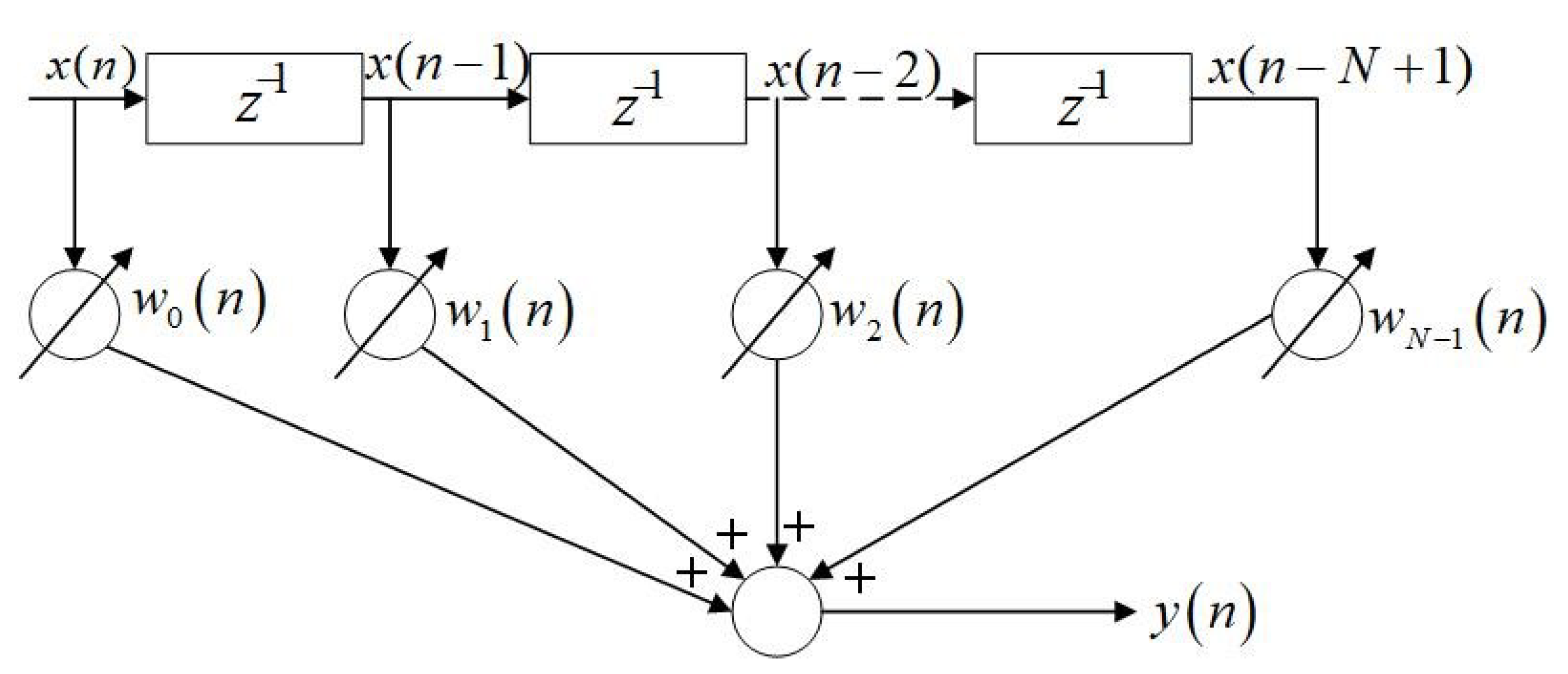
The LMS algorithm is used in an adaptive system to adjust the weight vector to change the system output timely in accordance with the variation in noise. An adaptive filter is a kind of linear combiner, and it is described in Figure 3.
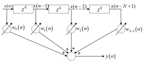
Figure 3.
Adaptive filter.
The constant input signal is divided into a series of discrete signals with time delay, and the quality of discrete signals is equal to that of the weighting coefficient, as shown as follows:
where T means transpose, is the time mark, and is the filter order. The weight vector is a significant component of the adaptive system, which can weigh the input signal and then form the output with a digital accumulator. The weight vector is given as:
The output is obtained as follows:
The error signal is defined as the desired signal subtracted from the filter output , which can be shown as:
The core of the adaptive algorithm is the method to adjust the weight vector. In this study, an adaptive filter with the LMS algorithm is applied in the adjustment of the weight vector. The purpose is to minimize the mean squared error (MSE) , which is given as:
From Equation (19), is a quadratic function about the weight coefficient vector. Therefore, Equation (19) has a unique minimum value, and the optimal weight vector can be gained at the minimum point. The approach to solving W is the steepest descent method, which makes the change in each step of the weight vector proportional to the negative value of the gradient vector and reaches the optimal solution along the shortest path. The iterative equation of the weight coefficient vector is described as follows:
where represents the next time of time n, and the gradient vector is given as:
where is the convergence coefficient.
3.2. Adaptive Control Termination with the LMS Algorithm
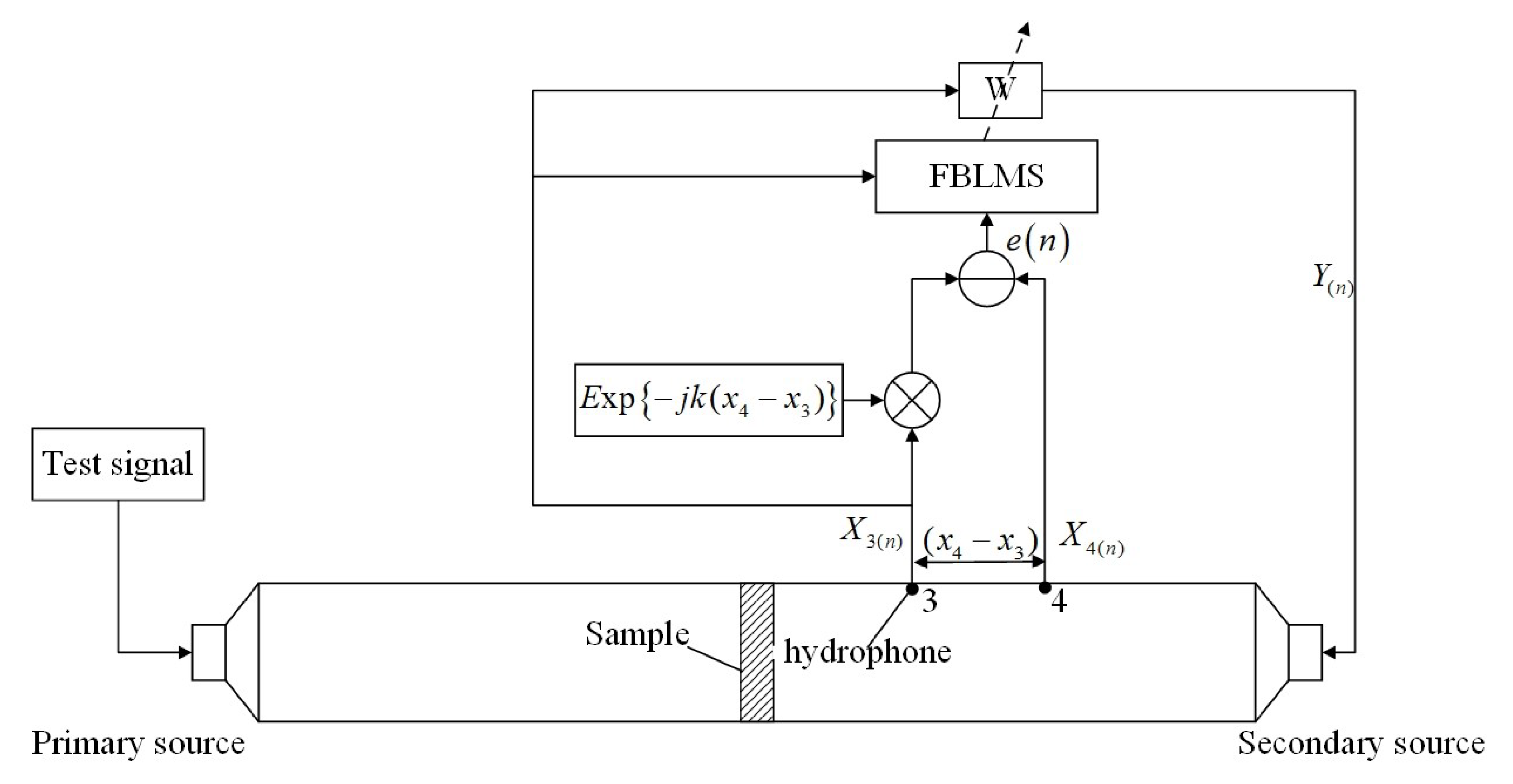
To express the working process of the adaptive algorithm for cancellation of the transmission-reflection wave, the signal-handling process is expressed in the frequency domain, as shown in Figure 4.
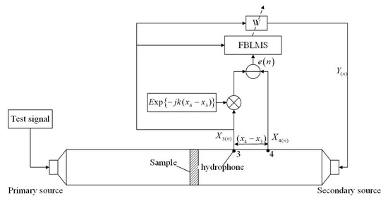
Figure 4.
Signal-handling process of adaptive control system.
The adaptive algorithm principle is driving the signal in the next time in accordance with the signal in the last moment. Hence, the subscript in bracket is the time mark. The output of termination at frequency downstream from Equation (17) can be shown as:
The signal at hydrophones 3 and 4 can be expressed as:
where is the primary source signal, is the actual transfer function between the primary source and hydrophone 3, and is the actual transfer function between adaptive termination and hydrophone 3. is the transfer function between the primary source and hydrophone 4, and is the transfer function between adaptive termination and hydrophone 4. Then, the error signal is given as:
where k is the complex wave-number, which can be obtained by , where is the sound frequency and c is the sound velocity. MSE can be given as:
The refreshment method of the weighting vector is the steepest descent method, and the iterative equation of the weight coefficient vector in this algorithm can be described as:
and the algorithm gradient can be obtained from
Although the above equations for deriving the correct weight vector utilize transfer functions, such as , and , we do not need to measure these transfer functions in actual application. We can obtain the error signal and input of the LMS algorithm through hydrophones 3 and 4 without measuring the transfer functions, which prevents the error caused by inaccurate transfer functions.
4. Simulation
4.1. Establishment of a Sound Tube Simulation Model
In this study, the COMSOL software is used for the simulation of adaptive control for an impedance tube to form a traveling wave downstream. A 3D model of impedance tube is established. The radius of the sound tube is 0.1 m, and its length is 5 m. Two excited sources exist on both sides of the impedance tube. They are the primary source (on the left) and the secondary sound source (on the right) with sizes of 0.1 m (radius) and 0.02 m (thickness).The material of the two sound sources is steel AISI 4340, which density is 7850 kg/, the Young modulus is 205 × , and the Poisson’s ratio is 0.28. The medium in the tube is water. The grid cell size is extremely fine. The physical field of the impedance tube inside is defined as pressure acoustic, and the physical fields of the primary and secondary sources are defined as solid mechanics. The interface between solid mechanics and pressure acoustic is the acoustic–structure coupling boundary.
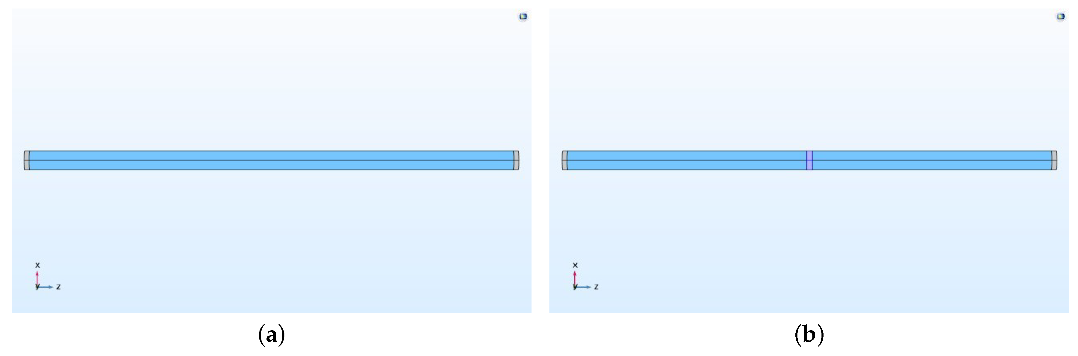
The adaptive algorithm is verified in two different models through simulation. One is a water-filled impedance tube without sample (water, with density of 1000 kg/ and sound velocity of 1500 m/s), and the other is a water-filled impedance tube with test sample (steel, with density of 7700 kg/ and sound speed of 6100 m/s). The sample thickness is 0.06 m.The wavelength the two models are shown in Figure 5.
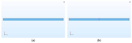
Figure 5.
(a) 3D model of impedance tube without sample in software. (b) 3D model of impedance tube with steel sample in software.
4.2. Procedure for Forming a Transmission-Traveling Wave Field
The second phase is to verify whether the adaptive algorithm helps the impedance tube form a traveling wave field in the transmission section successfully or not by controlling the secondary source. The frequency range tested in the simulation is 100–2500 Hz. The wavelength calculation equation is as follow:
where is wavelength, c is the sound speed, and f is frequency. The range of wavelength in water is from 0.6 m to 15 m, and the range of wavelength in steel is from 2.44 m to 61 m. Owing to the page limitation, only the sound field of the transmission section (before and after control of the adaptive algorithm) in the frequency of 2500 Hz and the transformation of the sound signals of hydrophones 3 and 4 in the above two working conditions (without sample and with steel sample) are displayed.
Initially, with the primary sound source working alone, the acoustic information (sound pressure amplitude and phase in the transmission section) can be collected in the transmission section, whose detailed information is shown in Figure 6 and Figure 7.
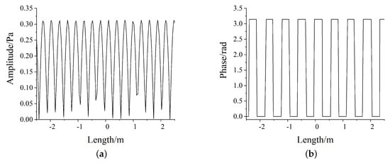
Figure 6.
(a)The information of sound pressure amplitude in impedance tube downstream without sample at 2500 Hz. (b) The information of sound pressure phase in impedance tube downstream without sample at 2500 Hz.
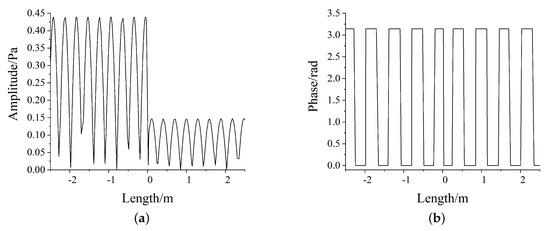
Figure 7.
(a) The information of sound pressure amplitude in sound tube inner with steel sample at 2500 Hz. (b) The information of sound pressure phase in sound tube inner downstream with steel sample at 2500 Hz.
The sound field style is a standard standing wave field. The acoustic information (amplitude and phase) is verified as the tube length in the figure when the primary source works alone.
Next, the secondary source begins to work with the adaptive algorithm. The output varies with time until the error signal in the adaptive algorithm is minimized to zero. The transformation of sound signals from hydrophones 3 and 4 can be achieved, as shown in Figure 8 and Figure 9.
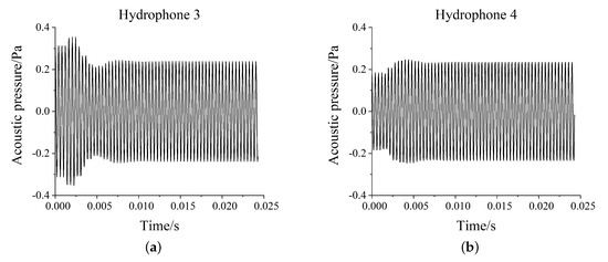
Figure 8.
(a)The signal of hydrophone 3 changes with time in the impedance tube without sample at 2500 Hz. (b) The signal of hydrophone 4 changes with time in the impedance tube without sample at 2500 Hz.
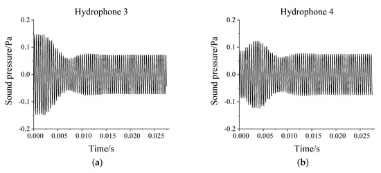
Figure 9.
(a) The signal of hydrophone 3 changes with time in the impedance tube with steel sample at 2500 Hz. (b) The signal of hydrophone 4 changes with time in the sound tube with steel sample at 2500 Hz.
Lastly, the acoustic information of the sound tube is collected again. The secondary source output is kept stable, as shown in Figure 10 and Figure 11.
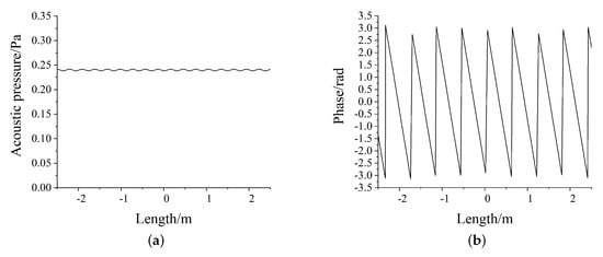
Figure 10.
(a) The information of sound pressure amplitude in sound tube inner with steel sample at 2500 Hz. (b) The information of sound pressure phase in sound tube inner with steel sample at 2500 Hz.

Figure 11.
(a) The information of sound pressure amplitude in sound tube inner with steel sample at 2500 Hz. (b) The information of sound pressure phase in sound tube inner with steel sample at 2500 Hz.
The adaptive algorithm applied to the water-filled sound tube to generate a traveling wave is demonstrated to be effective through comparing the above acoustic information in the transmission section before and after controlling by using the adaptive algorithm. By comparing Figure 7 and Figure 11, it can be observed that the variation of sound field distribution in water before and after the adaptive control in transmission section. Before the adaptive active control, the sound field changes dramatically with distance, which is close to standing wave field. After control, the sound field fluctuates in a very small range, which is almost a traveling wave field in the downstream of tube.
4.3. Simulation Results
The last steps are collecting the data of locations where hydrophones 1, 2, 3, and 4 lie in and calculating the reflection coefficient (R) and transmission coefficient (T) by using Equations (7) and (8) in two different working conditions.
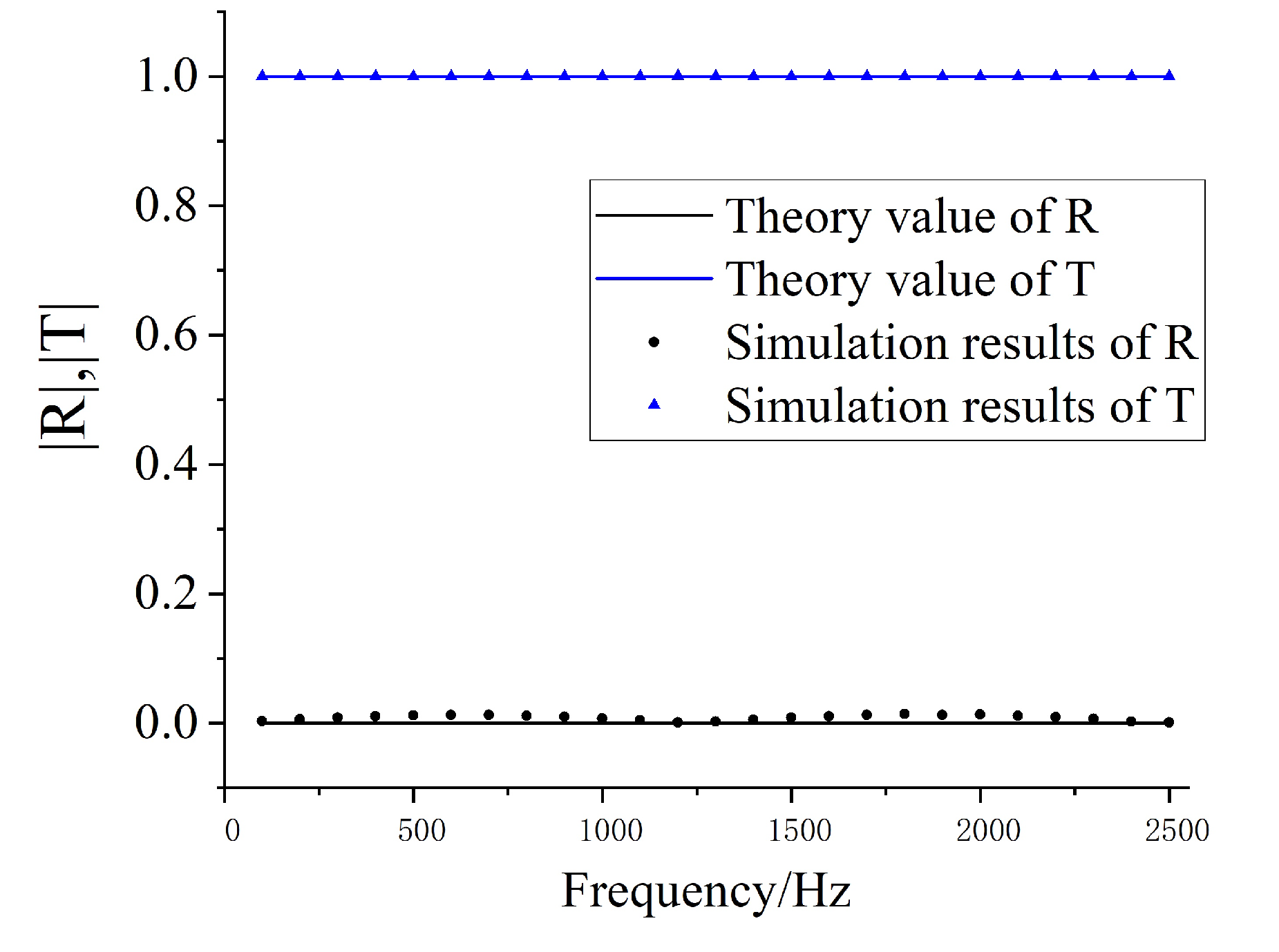
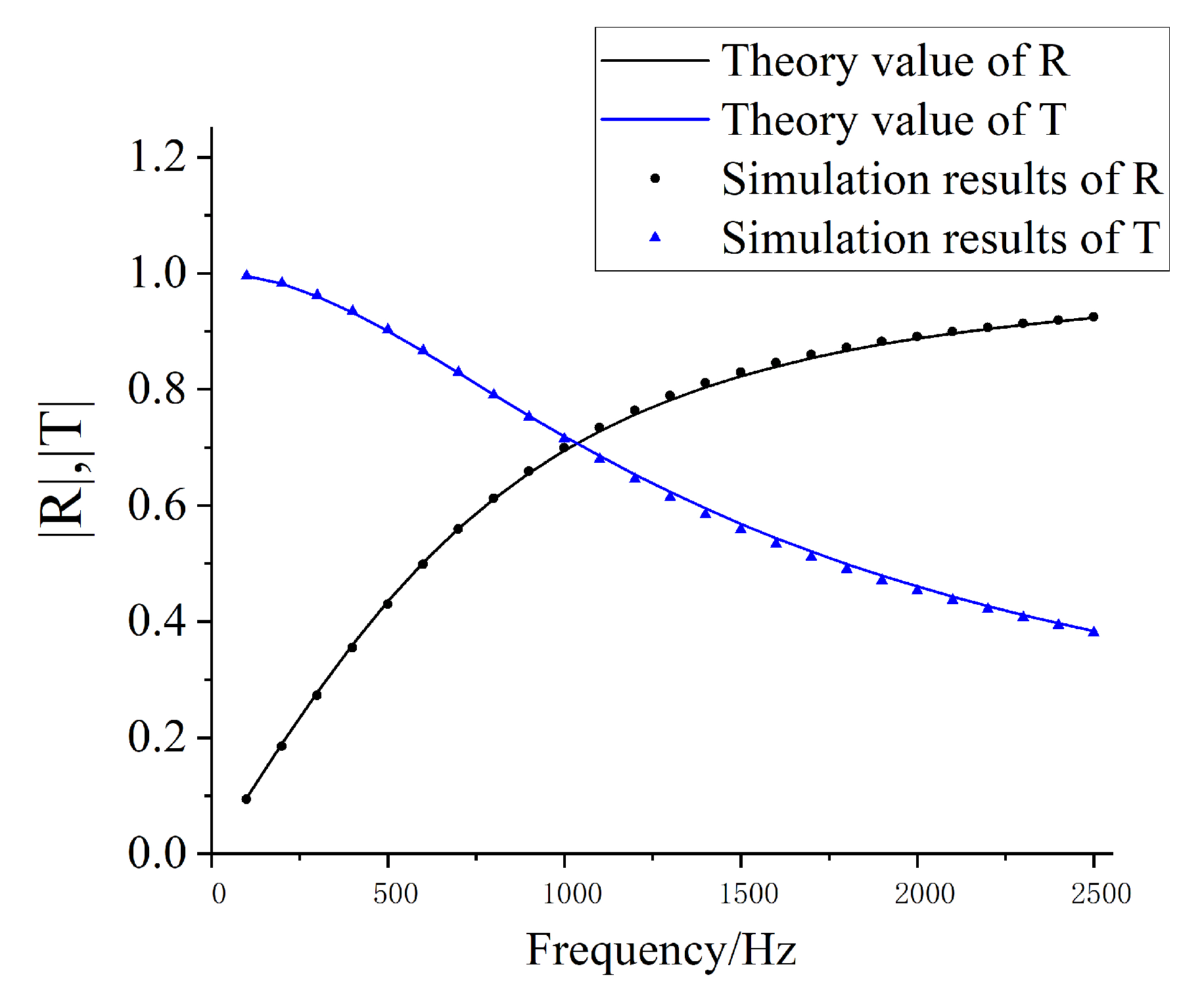
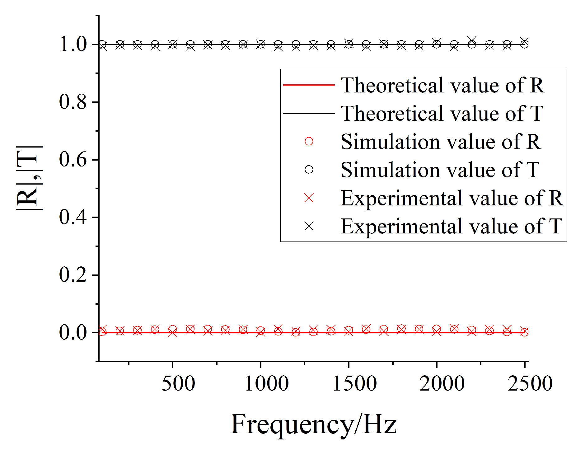
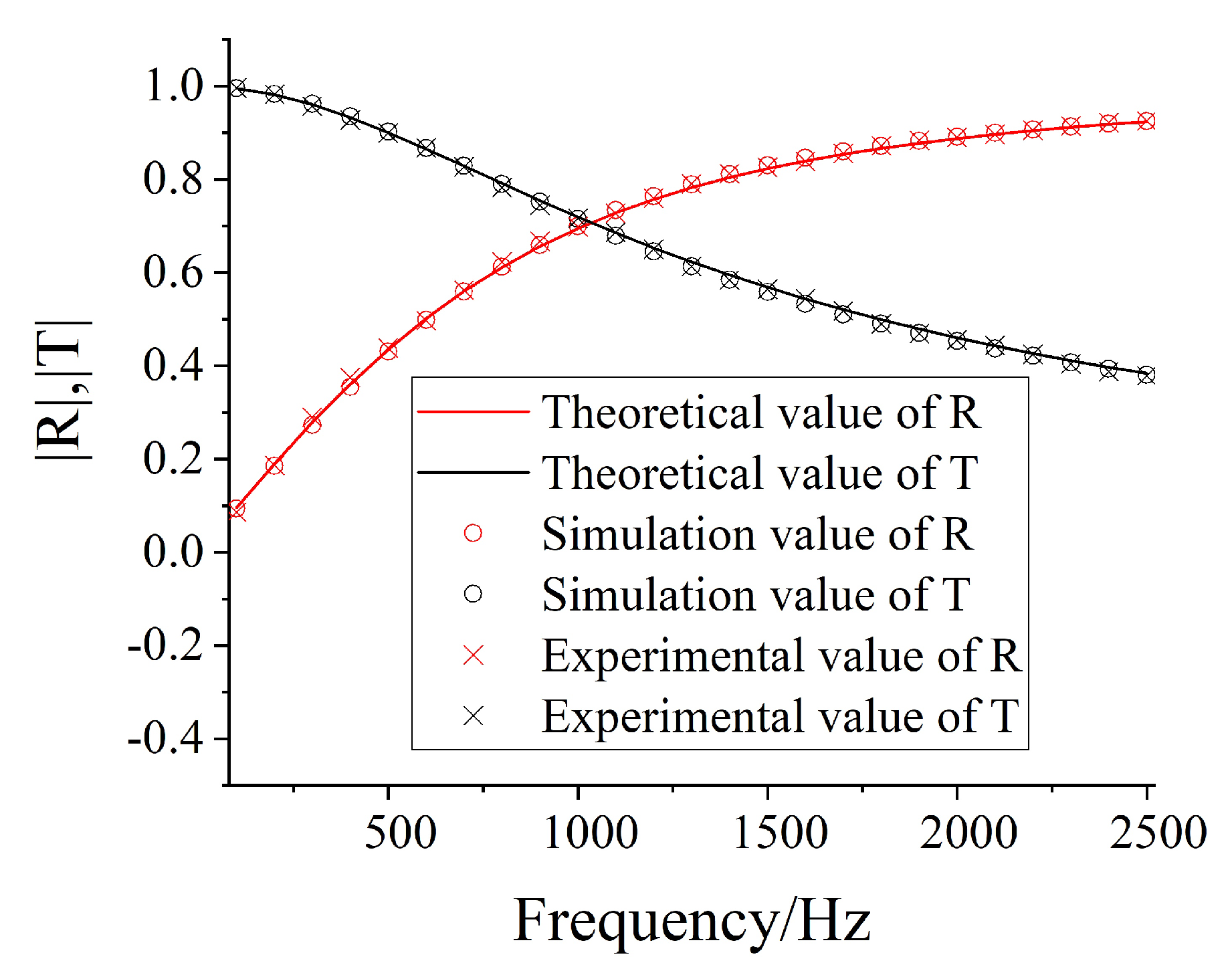
For the impedance tube without sample, a reflection wave does not exist, leaving only incident waves. Therefore, the theoretical values of the reflection and transmission coefficients are 0 and 1, respectively. The theoretical value of the sample (steel) can be calculated in accordance with Literature [42]. Then, the theoretical value and the calculated results in the two conditions are compared, as shown in Figure 12 and Figure 13.

Figure 12.
Comparison of the theoretical and the simulation values of reflection coefficient (R) and transmission coefficient (T), when there is no sample in the impedance tube.

Figure 13.
Comparison of the theoretical and the simulation values of reflection coefficient (R) and transmission coefficient (T), when there is a steel sample in the impedance tube.
5. Experimental Implementation
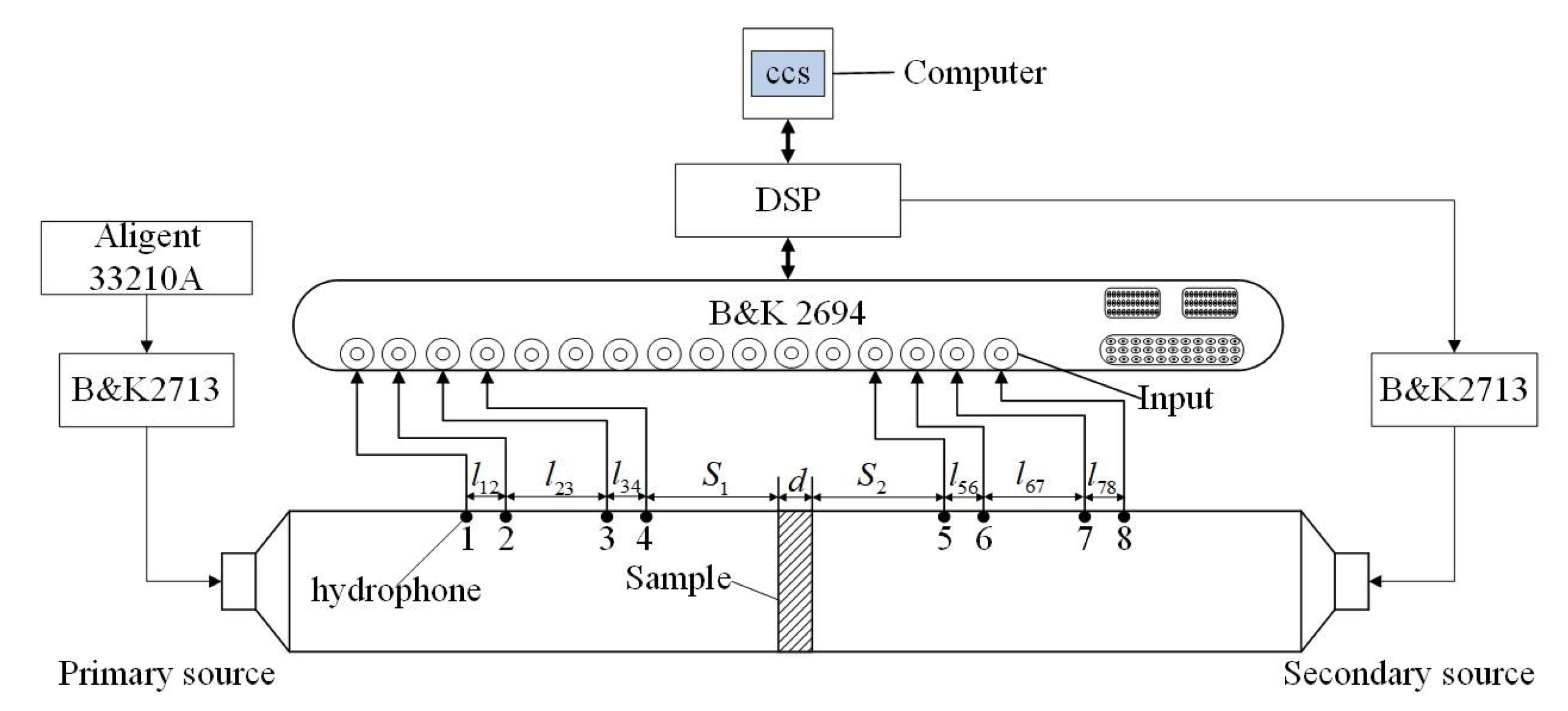
The experimental apparatus connected is shown in Figure 14. The inner diameter of the sound tube is 208 mm, the outer diameter is 416 mm, and the length is 5 m. Two underwater low-frequency acoustic projectors act as the primary and secondary sources. Eight hydrophones (B&K 8103, with sensitivity of 19.9 UV/Pa) within the sound tube are placed on both sides of the sample. Four of the hydrophones are placed on the left side to separate incident and reflection waves. The four other hydrophones on the right side are used for providing input signals of the adaptive control system and verifying whether the formation of a transmission-traveling wave downstream of the impedance tube is successful or not.
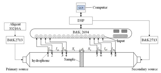
Figure 14.
Experimental instrument connection diagram.
With the test frequency changes, the combination of different hydrophones is selected. The distance between hydrophones and the distance from hydrophones to the surface of sample are shown in Table 1. When the test frequency range is 100–750 Hz, selecting hydrophones 2, 3, 6, and 7 as the signal input of the adaptive system, and for the test frequency range is 750 to 2500 Hz, the combination selected is hydrophones 1, 2, 7, and 8.

Table 1.
The distance between hydrophones and the distance from hydrophones to the surface of sample.
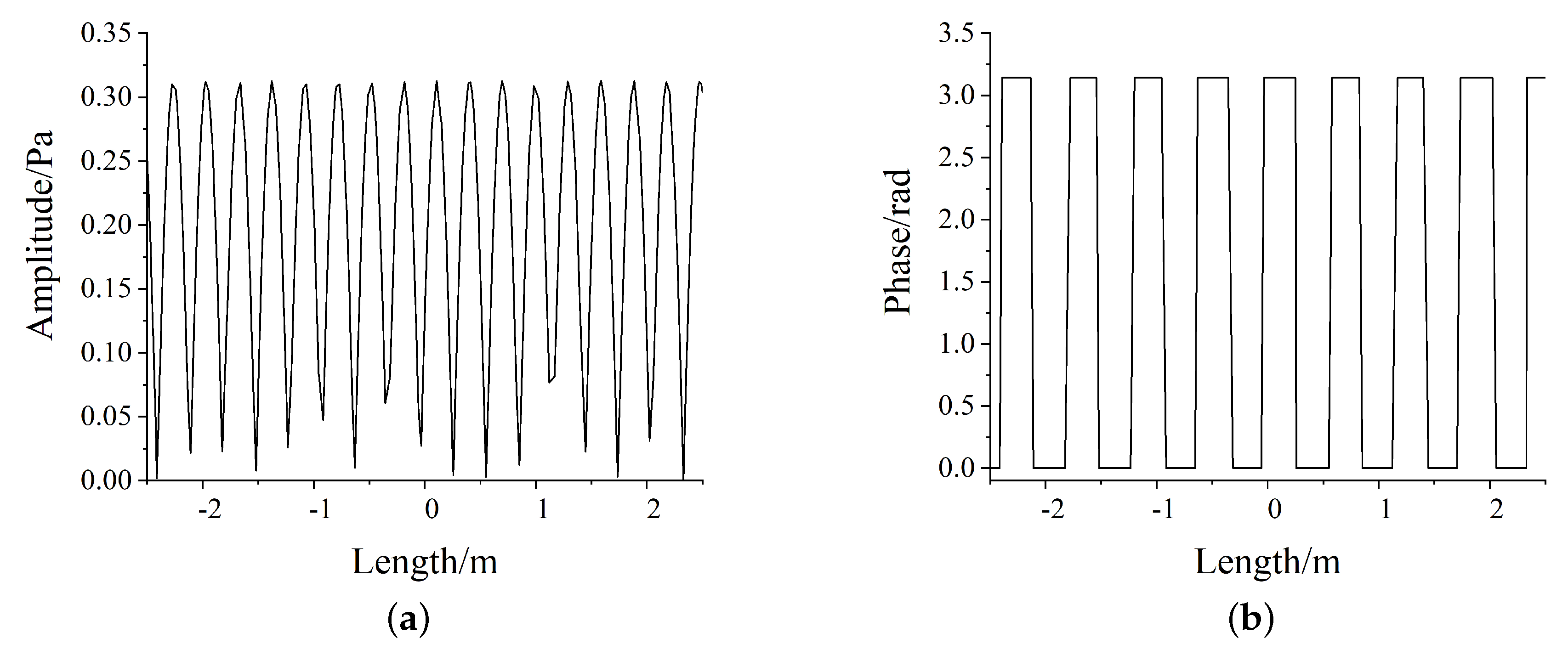
First, we control a waveform generator (Agilent 33210A) to generate a continuous plane wave signal with certain frequency and amplitude, which is amplified using a power amplifier (B&K 2713) to excite the primary sound source. Then, the acoustic pressure information detected using the six hydrophones after passing through the measurement amplifier (B&K 2694) is transferred into a digital signal processing (DSP) board. The acoustic pressure signal amplified using hydrophones 3 and 4 is sent into the adaptive control algorithm in the DSP board to compute the proper exciting signal to cancel the transmission–reflection wave (D). The adaptive algorithm implemented in the DSP board can be programmed in the code composer studio (CCS) software on a computer. The outputs of the six hydrophones, set as the inputs for the DSP board and their sound pressure information, can be displayed in the CCS of the computer. When the output of the secondary source is kept stable, the computer collects the acoustic pressure information of the four hydrophones downstream again to observe the ideal degree of the transmission–traveling wave field. The output amplitude of the waveform generator is set as 1 Vpp, the amplification of the power amplifier (B&K2713) is set as 40dB, and the amplification of the measurement amplifier (B&K2694) is set as 10 dB. The primary and secondary sound sources are self-developed products of the same type which the resonant peak is about 30 kHz. The transmission voltage response is relatively flat in the experimental test frequency range 100 to 2500 Hz. In the test frequency range, when the test frequency is changed, the error function of the adaptive algorithm will minimize to 1 Pa in 5 s. Once the amplitude of error signal tends to zero and remains stable, collecting the sound field information in the tube. In this experiment, the threshold of the amplitude of error signal is set at 1 Pa. The relationship between acoustic pressure amplitude and phase and sound tube length in the frequency of 600 Hz is shown in Figure 15 and Figure 16.
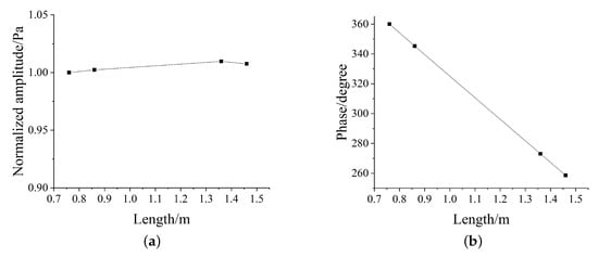
Figure 15.
(a) The relationship between acoustic pressure amplitude and impedance tube length without sample at 600 Hz. (b) The relationship between acoustic phase and impedance tube length without sample at 600 Hz.
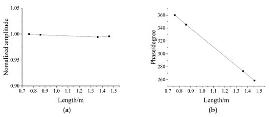
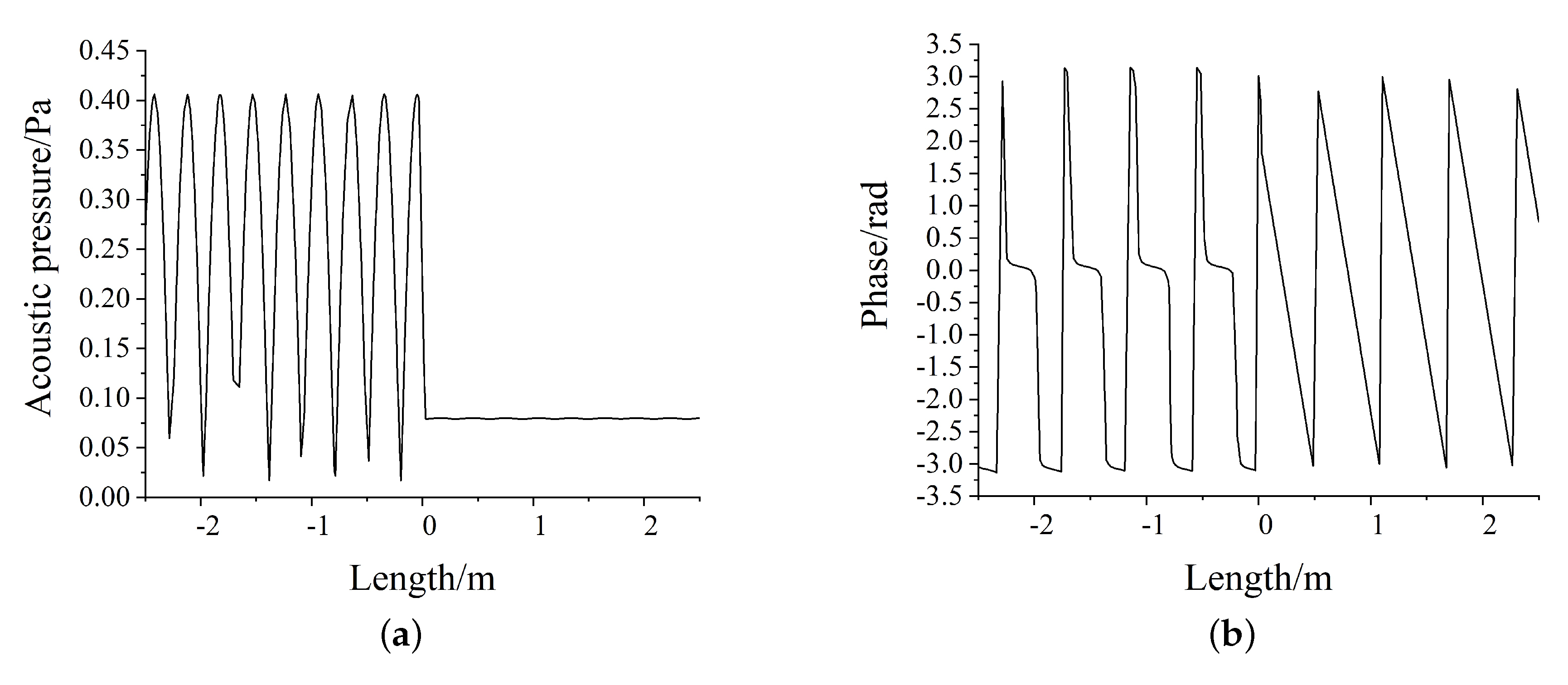
Figure 16.
(a) The relationship between acoustic pressure amplitude and impedance tube length with steel sample at 600 Hz. (b) The relationship between acoustic phase and impedance tube length with steel sample at 600 Hz.
When a transmission–traveling wave is formed, the reflection coefficient (R) and transmission coefficient (T) will be obtained in accordance with Equations (7) and (8). The results are displayed in Figure 17 and Figure 18.
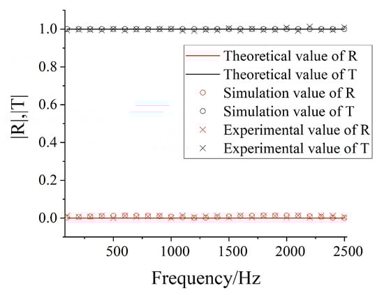
Figure 17.
Comparison of the theoretical, the simulation values and experimental values of reflection coefficient (R) and transmission coefficient (T), when there is no sample in the impedance tube.
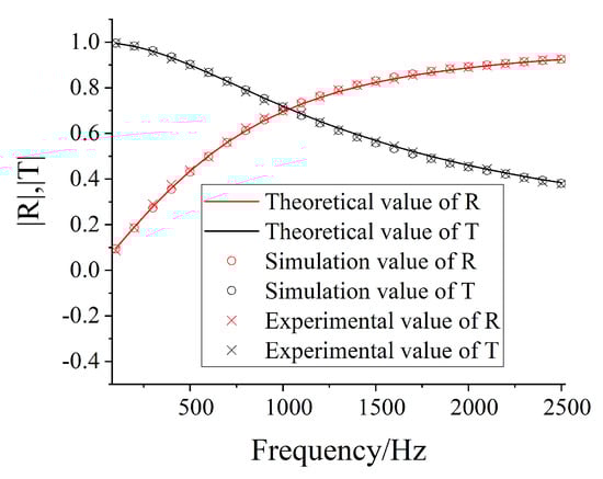
Figure 18.
Comparison of the theoretical, the simulation values and experimental values of reflection coefficient (R) and transmission coefficient (T), when there is a steel sample in the impedance tube.
6. Conclusions
The wavelength in water becomes longer with the frequency decreasing, which cause it is difficult to measure and remove the reflected wave from the end of the sound tube with traditional methods, so the reflection coefficient and transmission coefficient of the underwater material at low frequencies cannot be accurately measured. However, The adaptive algorithm in this paper can effectively remove the transmission-reflected waves at low frequencies, and accurately measure the reflection coefficient and transmission coefficient of the test sample. This work proves that the adaptive control termination of an sound tube can help form traveling waves downstream of the tube, and the reflection and transmission coefficients of sample can be calculated automatically and accurately. It confirms the achievable line of the theory from three steps: theory, simulation, and experiment.
First, adaptive control theory of a transmission sound field is proposed through the analysis of the characters of an impedance tube and research on the LMS algorithm.
Second, a physical model that conforms to a real impedance tube is built in the COMSOL simulation software, and a real intratube environment is simulated. The acoustic information of the inner part of the sound tube is extracted before and after control using the adaptive method. The successful establishment of transmission–traveling waves downstream of the tube is proven through comparing the sound field downstream of the impedance tube between control on and off. The effectiveness of the adaptive method is also verified.
Lastly, the experimental results demonstrate that transmission–traveling waves are formed successfully by extracting the sound pressure information of four hydrophones downstream of the impedance tube. The trend of the curve of the reflection and transmission coefficients of the sample calculated using a computer is consistent with the theoretical curve, with a minor difference.
The advantage of the TWT adaptive control method over the transfer function method includes that the adaptive control method can avoid multiple repetitive operations while changing the test frequency. Moreover, the reflection and transmission coefficients of the sample can be calculated simultaneously through the adaptive control system, and the absolute error of the measurement result is less than 0.02. By contrast, the transfer function method cannot do it.
Author Contributions
Methodology, Y.X., X.Z.; software, X.Z.; validation, Y.X.; formal analysis, Y.X.; writing—original draft preparation, Y.X.; writing—review and editing, X.Z., Y.X.; supervision, Y.X. All authors have read and agreed to the published version of the manuscript.
Funding
This research work was funded by Natural Science Foundation of Heilongjiang Province (LH2020A009).
Institutional Review Board Statement
Not applicable.
Informed Consent Statement
Not applicable.
Data Availability Statement
Not applicable.
Acknowledgments
The authors would like to thank the College of Underwater Acoustic Engineering Laboratory.
Conflicts of Interest
The authors declare no conflict of interest.
References
- Ting, R. Characterization of the properties of underwater acoustical materials. J. Acoust. Soc. Am. 1989, 86, S21–S22. [Google Scholar] [CrossRef] [Green Version]
- Taylor, H.O. Tube Method of Measuring Sound Absorption. J. Acoust. Soc. Am. 1952, 24, 701–704. [Google Scholar] [CrossRef]
- Chung, J.; Blaser, D.A. Transfer function method of measuring in-duct acoustic properties. I—Theory. II—Experiment. J. Acoust. Soc. Am. 1980, 68, 907–921. [Google Scholar] [CrossRef]
- Hirosawa, K.; Takashima, K.; Nakagawa, H.; Kon, M.; Yamamoto, A.; Lauriks, W. Comparison of three measurement techniques for the normal absorption coefficient of sound absorbing materials in the free field. J. Acoust. Soc. Am. 2009, 126, 3020–3027. [Google Scholar] [CrossRef]
- Wilson, P.; Roy, R.; Carey, W.M. An improved water-filled impedance tube. J. Acoust. Soc. Am. 2003, 113, 3245–3252. [Google Scholar] [CrossRef] [PubMed]
- Sun, L.; Hou, H.; Dong, L.; Wan, F.R. Measurement of characteristic impedance and wave number of porous material using pulse-tube and transfer-matrix methods. J. Acoust. Soc. Am. 2009, 126, 3049–3056. [Google Scholar] [CrossRef] [PubMed]
- Mongeau, L.; Thompson, D.E. Application of the transfer function method to acoustic measurements in a duct with flow. J. Acoust. Soc. Am. 1990, 87, S34. [Google Scholar] [CrossRef]
- Tyutekin, V.V. Precision of the material parameter measurements in the acoustic low-frequency pipe. Acoust. Phys. 2001, 47, 746–754. [Google Scholar] [CrossRef]
- Finneran, J.J.; Hastings, M. Active Impedance Control in a Water-Filled Waveguide for Low-Frequency Bioacoustic Testing. J. Acoust. Soc. Am. 1997, 102, 3196–3197. [Google Scholar] [CrossRef]
- Piquette, J.; Forsythe, S.E. Low-frequency echo-reduction and insertion-loss measurements from small passive-material samples under ocean environmental temperatures and hydrostatic pressures. J. Acoust. Soc. Am. 2001, 110, 1998–2006. [Google Scholar] [CrossRef]
- Park, C.M.; Ih, J.G.; Nakayama, Y.; Takao, H. Inverse estimation of the acoustic impedance of a porous woven hose from measured transmission coefficients. J. Acoust. Soc. Am. 2003, 113, 128–138. [Google Scholar] [CrossRef] [PubMed]
- Bolleter, U.; Chanaud, R. Modal Analysis of Sound Propagation in a Circular Duct and Application to In-Duct Sound Measurements. J. Acoust. Soc. Am. 1970, 47, 116. [Google Scholar] [CrossRef]
- Bishop, D. Small Reverberation Chamber for Measuring the Sound Absorption of Materials at High Frequencies. J. Acoust. Soc. Am. 1955, 27, 1003. [Google Scholar] [CrossRef]
- Sabine, P.E. Measurements in the Reverberation Chamber. Acoust. Soc. Am. 1939, 11, 159–160. [Google Scholar] [CrossRef]
- Sato, S.; Fujimori, T.; Miura, H. An estimation of absorption coefficients measured in a small reverberation chamber. J. Acoust. Soc. Am. 1988, 84, S95–S96. [Google Scholar] [CrossRef]
- Hardy, H.C.; Tyzzer, F. Experimentation on the Theory of the Reverberation Method of Measuring Acoustical Absorption. J. Acoust. Soc. Am. 1952, 24, 115. [Google Scholar] [CrossRef]
- Sun, L.; Hou, H. Transmission loss measurement of acoustic material using time-domain pulse-separation method (L). J. Acoust. Soc. Am. 2011, 129, 1681–1684. [Google Scholar] [CrossRef]
- Powell, J.G.; Houten, J.J.V. A Tone-Burst Technique of Sound-Absorption Measurement. J. Acoust. Soc. Am. 1970, 47, 80. [Google Scholar] [CrossRef]
- Cole, J.E.; Martini, K. Low-frequency impedance measuring device for underwater acoustic materials. J. Acoust. Soc. Am. 1994, 95, 2931. [Google Scholar] [CrossRef]
- Anderson, R.E.; Watson, R.B. Measurement of Sound Absorption Coefficients with Acoustic Pulses. J. Acoust. Soc. Am. 1957, 29, 178. [Google Scholar] [CrossRef] [Green Version]
- He, P. Measurement of acoustic dispersion using both transmitted and reflected pulses. J. Acoust. Soc. Am. 2000, 107, 801–807. [Google Scholar] [CrossRef] [Green Version]
- Ho, L.T.; Heiner, L.; Shrader, J.M. An impedance measuring facility for the low-frequency evaluation of acoustic materials. J. Acoust. Soc. Am. 1974, 56, S30. [Google Scholar] [CrossRef] [Green Version]
- Seybert, A. Two-sensor methods for the measurement of sound intensity and acoustic properties in ducts. J. Acoust. Soc. Am. 1988, 83, 2233–2239. [Google Scholar] [CrossRef] [Green Version]
- Finneran, J.J.; Hastings, M. Active impedance control within a cylindrical waveguide for generation of low-frequency, underwater plane traveling waves. J. Acoust. Soc. Am. 1999, 105, 3035–3043. [Google Scholar] [CrossRef]
- Orduña-Bustamante, F.; Nelson, P. An adaptive controller for the active absorption of sound. J. Acoust. Soc. Am. 1992, 91, 2740–2747. [Google Scholar] [CrossRef]
- Beatty, L.G. Acoustic Impedance in a Rigid-Walled Cylindrical Sound Channel Terminated at Both Ends with Active Transducers. J. Acoust. Soc. Am. 1964, 36, 1081–1089. [Google Scholar] [CrossRef]
- Sivian, L.J. Sound Propagation in Ducts Lined with Absorbing Materials. J. Acoust. Soc. Am. 1937, 9, 77. [Google Scholar] [CrossRef]
- Finneran, J.J.; Hastings, M. Active/passive technique for the creation of a low-frequency traveling wave inside a water- Filled tube. J. Acoust. Soc. Am. 1995, 98, 2941. [Google Scholar] [CrossRef]
- Shields, F.D.; Bass, H.; Bolen, L. Tube method of sound-absorption measurement extended to frequencies far above cutoff. J. Acoust. Soc. Am. 1977, 62, 346–353. [Google Scholar] [CrossRef]
- Cheung, W.; Jho, M.; Kim, Y. Improved Method for the Measurement of Acoustic Properties of a Sound Absorbent Sample in the Standing wave tube. J. Acoust. Soc. Am. 1995, 97, 2733–2739. [Google Scholar] [CrossRef]
- Hjerpe, E. Measurement of normal-incidence acoustic pressure reflection coefficient using one microphone at two fixed locations in a standing wave tube. J. Acoust. Soc. Am. 1993, 94, 1168. [Google Scholar] [CrossRef]
- McIntosh, J.D.; Zuroski, M.T.; Lambert, R. Standing wave apparatus for measuring fundamental properties of acoustic materials in air. J. Acoust. Soc. Am. 1990, 88, 1929–1938. [Google Scholar] [CrossRef]
- Anderson, A.; Hampton, L. Use of tubes for measurement of acoustical properties of materials. J. Acoust. Soc. Am. 1975, 57, S30. [Google Scholar] [CrossRef]
- Peng, D.L.; Hu, P.; Zhu, B. The modified method of measuring the complex transmission coefficient of multilayer acoustical panel in impedance tube. Appl. Acoust. 2008, 69, 1240–1248. [Google Scholar] [CrossRef]
- Bolton, J.; Yun, R.J.; Pope, J.; Apfel, D. Development of a New Sound Transmission Test for Automotive Sealant Materials. SAE Trans. 1997, 106, 2651–2658. [Google Scholar]
- Guicking, D.; Karcher, K. Active Impedance Control for One-Dimensional Sound. J. Vib. Acoust. Trans. ASME 1984, 106, 393–396. [Google Scholar] [CrossRef]
- Smith, J.; Johnson, B.; Burdisso, R. A broadband passive–active sound absorption system. J. Acoust. Soc. Am. 1999, 106, 2646–2652. [Google Scholar] [CrossRef] [Green Version]
- Robin, O.; Berry, A.; Doutres, O.; Atalla, N. Measurement of the absorption coefficient of sound absorbing materials under a synthesized diffuse acoustic field. J. Acoust. Soc. Am. 2014, 136, EL13–EL19. [Google Scholar] [CrossRef] [Green Version]
- Ciaburro, G.; Iannace, G. Numerical Simulation for the Sound Absorption Properties of Ceramic Resonators. Fibers 2020, 8, 77. [Google Scholar] [CrossRef]
- Machuca-Tzili, F.A.; Orduña-Bustamante, F.; Pérez-López, A.; Pérez-Ruiz, S.J.; Perez-Matzumoto, A.E. Modified acoustic transmission tube apparatus incorporating an active downstream termination. J. Acoust. Soc. Am. 2017, 141, 1093. [Google Scholar] [CrossRef]
- Kirkeby, O.; Nelson, P.; Hamada, H.; Orduña-Bustamante, F. Fast deconvolution of multichannel systems using regularization. IEEE Trans. Speech Audio Process. 1998, 6, 189–194. [Google Scholar] [CrossRef] [Green Version]
- Brekhovski. Wave in Multilayers; Science Press: Beijing, China, 1980; pp. 45–53. [Google Scholar]


Publisher’s Note: MDPI stays neutral with regard to jurisdictional claims in published maps and institutional affiliations. |
© 2021 by the authors. Licensee MDPI, Basel, Switzerland. This article is an open access article distributed under the terms and conditions of the Creative Commons Attribution (CC BY) license (https://creativecommons.org/licenses/by/4.0/).