Deep-Feature-Based Approach to Marine Debris Classification

Abstract

The global community has recognized an increasing amount of pollutants entering oceans and other water bodies as a severe environmental, economic, and social issue. In addition to prevention, one of the key measures in addressing marine pollution is the cleanup of debris already present in marine environments. Deployment of machine learning (ML) and deep learning (DL) techniques can automate marine waste removal, making the cleanup process more efficient. This study examines the performance of six well-known deep convolutional neural networks (CNNs), namely VGG19, InceptionV3, ResNet50, Inception-ResNetV2, DenseNet121, and MobileNetV2, utilized as feature extractors according to three different extraction schemes for the identification and classification of underwater marine debris. We compare the performance of a neural network (NN) classifier trained on top of deep CNN feature extractors when the feature extractor is (1) fixed; (2) fine-tuned on the given task; (3) fixed during the first phase of training and fine-tuned afterward. In general, fine-tuning resulted in better-performing models but is much more computationally expensive. The overall best NN performance showed the fine-tuned Inception-ResNetV2 feature extractor with an accuracy of $91.40\%$ and F1-score $92.08\%$, followed by fine-tuned InceptionV3 extractor. Furthermore, we analyze conventional ML classifiers’ performance when trained on features extracted with deep CNNs. Finally, we show that replacing NN with a conventional ML classifier, such as support vector machine (SVM) or logistic regression (LR), can further enhance the classification performance on new data.

1. Introduction

The rising level of marine pollution is a growing environmental problem in today’s society. Our oceans, seas, and other water bodies are polluted with various waste items that threaten coastal wildlife, habitat, human safety, and coastal communities’ economic health [1]. Discarded fishing gear continues to trap and kill marine life. Animals such as seabirds or turtles often mistake plastic debris with their food due to its similar appearance and odor, which leads to their malnutrition and starvation [2,3]. In addition, seafood contaminated with microplastics, i.e., small plastic particles less than 5 mm in size, is potentially toxic for humans that consume it [4,5,6]. Furthermore, marine debris induces high economic costs in industries such as tourism, aquaculture, and fisheries [7]. The key measures for solving marine pollution include detailed knowledge of magnitudes, sources, and impacts of marine debris, general behavioral change, enhancement of circular economy, prevention of waste items entering the marine environment, reducing waste generation, and removal of debris already present in the marine environment [8]. Identification and the cleanup of marine debris, especially one deep under the water surface, is challenging and expensive. Therefore, to make the cleanup process more efficient, automatized detection and removal of marine debris is desired. The latter can be realized with the aid of autonomous underwater vehicles (AUVs) and deep-learning-based visual identification of underwater waste.

Deep learning methods have been successfully utilized on various computer vision tasks, including object detection and localization [9,10], classification [11,12], and semantic segmentation [13,14]. Unlike conventional machine learning techniques, which require domain-specific hand-engineered feature extraction, deep learning techniques automatically learn hidden data representations from the raw data [15] and provide end-to-end learning mechanisms. Convolutional neural networks (CNNs) [16] are one of the leading methods contributing to the success of deep learning when it comes to image and video data. The architectural design of CNNs is inspired by receptive field structures in the animal visual cortex [17,18] and designed to learn features hierarchically by composing lower-level features into higher-level ones. The three main components of CNN architecture are convolutional, pooling, and fully connected layers. Feature maps are calculated by sliding convolutional kernels across all spatial locations using the predefined stride and computing dot-products between kernel’s weights and small local patches in the input volume. Each convolutional kernel produces one corresponding feature map. Lower convolutional layers extract generic features such as lines and edges, while higher layers encode more complex, higher-level features. Nonlinear activation function, usually rectified linear unit (ReLU) [19], is applied element-wise on obtained feature maps to introduce nonlinearity, which is desirable for detecting nonlinear features [20]. Pooling layers reduce the input’s spatial size by replacing local patches in input feature maps by their maximum or mean value to achieve invariance to small shifts and distorsions. Some CNN architectures add additional fully connected layers on top of the stacked convolutional and pooling layers before the final softmax layer [21,22] to perform high-level reasoning [20]. This paper addresses the problem of automatic, image-based marine debris classification and identification by utilizing the features extracted via existing state-of-the-art deep convolutional architectures.

In recent years, several works have employed deep-learning-based techniques to tackle the problem of marine debris detection, classification, and quantification. The study in [23] utilizes convolutional neural network architecture to identify marine debris in forward-looking sonar imagery autonomously. In [24], a single-stage RetinaNet detector trained on non-aquatic waste images is used to detect trash items in aquatic surroundings. Kylili et al. use VGG16 convolutional model architecture to automatically classify floating macro-plastic marine debris images in three categories (bottle, bucket, and straw) [25] and distinguish between six types of plastic debris, one type of marine life, and other items encountered at the shoreline or the seawater [26]. Fulton et al. [27] evaluate four different neural network architectures for visual detection of plastic debris in realistic underwater environments. Models were trained to detect three classes of objects in underwater videos: plastic, all man-made objects intentionally placed in the environment, and all biological material. Politikos et al. [28] use region-based CNN for the automated detection of seafloor marine litter on imaginary acquired in Ermoupolis bay, Syros Island, Greece. Musić et al. [29] carried an initial study out on the performance of neural networks for the detection and classification of underwater sea litter images trained and tested on a dataset built using images available from the Internet and hybrid images generated using a Blender environment from given background images and 3D litter models. In [30], machine learning techniques, including CNNs, are utilized to automatically classify images of five types of microplastic particles present on beaches in the Canary Islands. The quantification of marine debris on beaches by using unmanned aerial vehicles and deep learning techniques is discussed in [31,32].

Automatized identification of marine debris comes with many challenges. First, there are various types of marine debris, with significant in-class variations. For example, plastic bottles, bags, and cups have different shapes but belong to the same type of marine debris-plastics. Second, waste objects should be detected in various degradation phases, no matter the recording angle, water turbidity, or illumination. Moreover, training deep neural networks requires a large amount of annotated data. Acquisition of a sufficiently large and diverse dataset for image-based marine debris classification is expensive and not always feasible. A common and effective strategy to overcome a deficit of labeled training data is transfer learning, i.e., knowledge transfer from source to the desired target domain [33]. The idea is to reuse features learned by the network pre-trained on a very large dataset, such as the ImageNet [34] dataset, which contains 1.2 million training images from 1000 classes, on a new task of interest.

There are two common approaches to transfer learning: (1) using a pre-trained network as a fixed feature extractor [35,36]; (2) fine-tuning a pre-trained network’s weights on a target dataset [37,38]. In the first approach, the last, usually fully connected, part of the network is removed, while the remaining part (convolutional base) stays fixed during the training. On top of the fixed base used for feature extraction, a new classifier, either a new neural network or a conventional machine learning classifier such as a support vector machine or a logistic regression classifier, is added to learn underlying patterns from extracted features and discriminate data according to them. The fine-tuning approach uses the pre-trained network weights as a weight initialization scheme. During the training, these weights are updated by backpropagating errors from the target task into the base network to improve the final generalization performance on a new task of interest [37].

The successful employment of transfer learning has been reported on computer vision tasks from various domains, such as medical image analysis [39,40,41,42], agriculture [43,44], remote sensing [45,46], and the textile industry [47]. Transfer learning has been utilized in several works considering marine debris identification and classification. The VGG16 network pre-trained on the ImageNet dataset is used as a fixed feature extractor for plastic marine waste classification in [25,26]. In [24], object-detection-based transfer learning is applied on the proposed RetinaNet model with ResNet50 backbone to detect waste items in aquatic surroundings. Successful object detection networks, YOLOv2, Tiny-YOLO, Faster RCNN, and Single Shot MultiBox Detector (SSD), are fine-tuned in [27] for underwater detection of three classes of objects, including plastic marine debris. As a backbone for their Mask R-CNN architecture for seafloor litter detection, Politikos et al. [28] use MobileNetV1 architecture pre-trained on the COCO detection dataset.

The main goals of this study were to: (1) develop the model for autonomus marine debris identification and classification of different types of marine debris; (2) compare the performance of prominent deep convolutional architectures, including VGG19, InceptionV3, ResNet50, Inception-ResNetV2, DenseNet121, and MobileNetV2, on the task of marine debris classification; (3) investigate different schemes to utilize transfer learning for marine debris classification: fixed extraction of features, fine-tuning, and combination of both; (4) compare the performance of conventional machine learning classifiers trained on feature vectors extracted by deep convolutional architectures.

The rest of the paper is structured as follows. Section 2 describes materials and methods used in this study: dataset (Section 2.1), implemented deep convolutional architectures (Section 2.2), and machine learning algorithms (Section 2.3). Section 3 gives implementation details and experimental settings. Experimental results are presented in Section 4 and discussed in Section 5. In Section 6, concluding remarks and directions for future work are given.

2. Materials and Methods

2.1. Dataset

A large annotated dataset of underwater trash is needed to utilize a deep-learning approach for marine debris detection and classification. The Japan Agency for Marine-Earth Science and Technology (JAMSTEC) has made their Deep-sea Debris Database, which contains numerous marine debris videos and photos, available online to the public [48]. In our work, we used data from the Deep-sea Debris Database complemented with Google Images. Images were manually labeled and validated by one of the researchers. Each image was visually inspected prior to being added to the dataset. The final dataset contains 2395 images from six different classes: glass, metal, plastic, rubber, other trash, and no trash. Figure 1 provides a sample of images from the dataset.

To ensure that training and test sets have the same distribution of considered classes, available data are divided into a training set and a test set as follows: $20\%$ of the images from each class were set aside for the final model evaluation, while the remaining $80\%$ were left for training.

Table 1. Data distribution.

Class	Images	Trainig Set	Test Set
Glass	178	143	35
Metal	497	398	99
Plastic	700	560	140
Rubber	211	169	42
Other trash	390	312	78
No trash	419	336	83
∑	2395	1918	477

shows the class-wise distribution of data in the original dataset as well as in the training and test subsets.

2.2. Deep Convolutional Architectures

Compared to traditional computer vision techniques, deep convolutional networks provide better accuracy in image classification tasks. Furthermore, they also provide superior flexibility since they can be retrained using custom datasets and also require less human expert analysis and fine-tuning [49]. This section describes six deep CNN architectures utilized in this work for marine debris classification and extraction of dense image representations.

The main components repeated through the following architectures are convolutional and spatial pooling layers: max pooling, average pooling, and global average pooling. Convolutional layers convolve the input with the kernel shared across all input’s spatial locations to obtain feature maps. The feature map value at position $(i,j)$ obtained with $k^{th}$ kernel (filter) is calculated as $z_{i,j,k}={\mathit{w}}_k^T{\mathit{x}}_{i,j}+b_k$, where ${\mathit{w}}_k$ and $b_k$ denote $k^{th}$ kernel’s weight vector and bias term, while ${\mathit{x}}_{i,j}$ denotes the input patch centered at $(i,j)$. The nonlinear activation function $g:\mathbb{R}\to \mathbb{R}$ is applied element-wise on obtained feature maps to obtain activations $a_{i,j,k}=g\left(z_{i,j,k}\right)$ [20]. The pooling layers aggregate information within feature map ${\mathit{a}}_k$ by replacing local pooling regions ${\mathcal{R}}_{i,j}$ in ${\mathit{a}}_k$ with the maximum element from ${\mathcal{R}}_{i,j}$ in the case of max pooling, and with arithmetic mean of elements in ${\mathcal{R}}_{i,j}$ in the case of average pooling. On the other hand, global average pooling averages all values in ${\mathit{a}}_k$.

2.2.1. VGG19

Simonyan et al. [22] proposed several deep configurations of CNN architecture with a different number of weight layers. These architectures, known as VGGNets, stack convolutional layers with small $3\times 3$ receptive fields in blocks followed by a max-pooling layer. In one network configuration, they utilize $1\times 1$ convolutions to increase the nonlinearity of the decision function without changing the receptive fields of convolutional layers. In this work, we employ VGG19 architecture that has 19 weight layers. The VGG19 architecture with $\approx 143.47$ M trainable parameters, as defined in [22], is illustrated in Figure 2.

2.2.2. InceptionV3

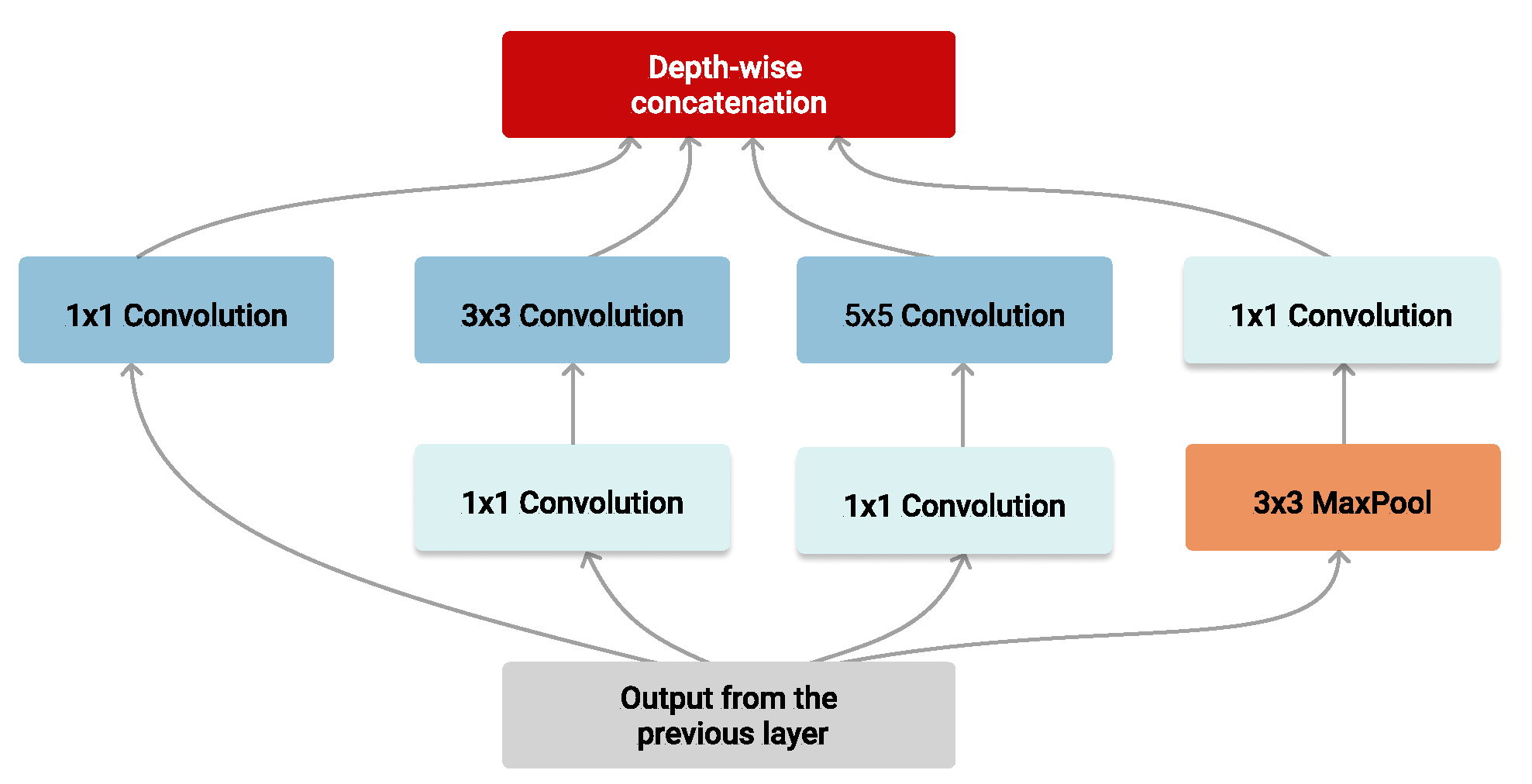
Although compellingly architecturally simple and with good generalization performance, VGGNets come with high computational costs. To obtain an efficient deep model with reduced computational costs and high generalization ability, Szegedy et al. stack Inception modules in a 22 weight layer deep GoogLeNet architecture [50]. In contrast to conventional architectures where either convolution (with a single filter size) or pooling operation is performed, Inception modules perform convolution with different filter sizes ($1\times 1$, $3\times 3$ and $5\times 5$) in parallel along with the max-pooling operation and pass the concatenated results forward throughout the network. Varying filter sizes enable the model to capture spatial information at different scales at the same level in the network. The computational efficiency is preserved by adding an extra $1\times 1$ convolution before expensive $3\times 3$ and $5\times 5$ convolutions and after the pooling layer, as illustrated in Figure 3. Two auxiliary classifiers are connected to intermediate Inception modules to propagate gradients through all network layers effectively.

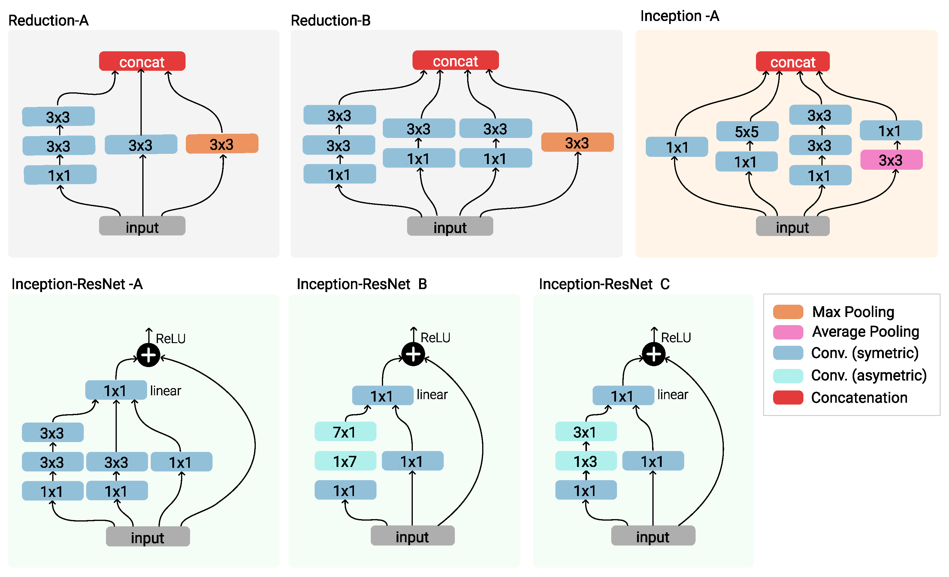
A later variant of the GoogLeNet architecture employed in this study, InceptionV3 architecture [51], modifies the original one in the following ways: (1) larger convolutions in the Inception modules are factorized into smaller ones, i.e., $5\times 5$ convolution is replaced by two $3\times 3$ convolutions in the Inception module A; (2) Inception module B factorizes symmetric $7\times 7$ convolutions into asymetric $1\times 7$ and $7\times 1$ convolutions; (3) the Inception module C, which is introduced for promotion of high dimensional representations, replaces $3\times 3$ convolution with parallel asymmetric $1\times 3$ and $3\times 1$ convolutions; (4) one auxiliary classifier with employed batch normalization is used as a regularizer together with the label smoothing technique; (5) efficient size reduction with parallel convolutional and pooling blocks with a stride two is employed in the reduction modules. Figure 4 and Figure 5 show modules and schematic representation of the InceptionV3 architecture. All convolutional layers employ batch normalization and use the ReLU activation function.

2.2.3. ResNet50

In [52], He et al. address the training accuracy degradation problem in deep network architectures by introducing the residual learning framework. Let $f\left(\mathit{x}\right)$ be the underlying mapping to be learned with several network layers, where $\mathit{x}$ denotes the input to the first of these layers. In the residual learning framework, stacked network layers learn the residual mapping $f_R\left(\mathit{x}\right):=f\left(\mathit{x}\right)-\mathit{x}$, which is easier to optimize than underlying $f\left(\mathit{x}\right)$. Original mapping $f\left(\mathit{x}\right)$ now corresponds to $f_R\left(\mathit{x}\right)+\mathit{x}$, which is realized with shortcut connections and element-wise additions in a feedforward convolutional network.

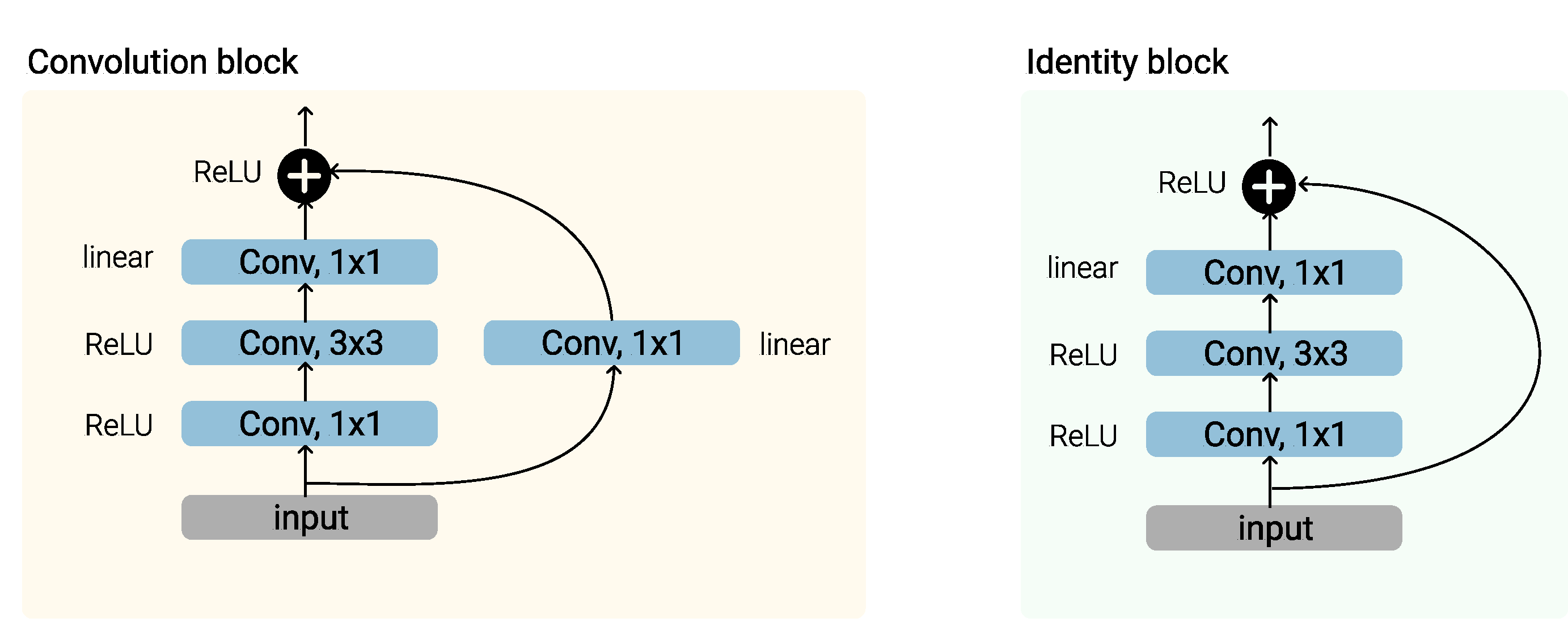
Residual Networks (ReNets) employ shortcut connections together with the batch normalization technique (after each convolution and before activation) to ease the training of deep network architectures and enjoy accuracy gains from an increase in network depth. Figure 6 shows two main residual modules, Convolution and Identity blocks, which comprise the 50/101/152 ResNet framework.

Identity shortcuts in identity blocks can only be used when input and output have the same dimension. Otherwise, a projection shortcut with $1\times 1$ convolutions, i.e., convolution block from Figure 6, is used to match the input and output dimensions. The 50-layers deep ResNet50 architecture employed in this study is illustrated in Figure 7.

2.2.4. Inception-ResNetV2

The Inception-ResNet [53] architecture combines good performing Inception architecture [51] with residual learning framework [52] by replacing the filter concatenation stage in Inception modules with residual connections. In residual versions of Inception modules (Inception-ResNet A, B and C modules in Figure 8), $1\times 1$ convolution without activation, i.e., with linear activation $g\left(x\right)=x$, is added before the summation to scale up the dimensionality of a given volume to match the input depth.

The batch normalization is utilized only on the top of traditional layers, not on summations. Introduction of residual connections into Inception architecture significantly accelerates the training of the Inception networks with an increased depth. However, the residual version of the Inception network is prone to instabilities during the training when a number of filters exceed 1000. To stabilize the training procedure, Inception-ResNets scale down the residuals before addition. Schematic representation of the Inception-ResNetV2 network architecture is shown in Figure 9.

2.2.5. DenseNet121

Huang et al. in [54] address the vanishing gradient problem of deep convolutional networks by introducing new, dense connectivity pattern in Densely Connected Convolutional Network (DenseNet) architecture. The main idea is to connect all layers directly with each other in a feed-forward manner to improve the information and gradient flow between layers as illustrated in Figure 10. The $m^{th}$ layer $L_m$ receives the original input ${\mathit{x}}_0$ and outputs ${\mathit{x}}_1,\dots ,{\mathit{x}}_{m-1}$ of all preceding layers $L_1,\dots ,L_m$ as input and outputs ${\mathit{x}}_m=f_m\left([{\mathit{x}}_0,{\mathit{x}}_1,\dots ,{\mathit{x}}_{m-1}]\right)$, where $[{\mathit{x}}_0,{\mathit{x}}_1,\dots ,{\mathit{x}}_{m-1}]$ denotes the depth-wise concatenation of volumes ${\mathit{x}}_0,{\mathit{x}}_1,\dots ,{\mathit{x}}_{m-1}$ (it is assumed that all volumes have the same width and height). If each layer outputs g feature maps and if d denotes the depth (number of channels) of input, then layer $L_m$ receives the input volume $[{\mathit{x}}_0,{\mathit{x}}_1,\dots ,{\mathit{x}}_{m-1}]$ of depth $d+(m-1)g$ and forwards a total of $d+mg$ feature maps to the next layer.

The architecture of densely connected network with 121 weight layers (excluding batch normalization layers), DenseNet121, is shown in Figure 11.

Four dense blocks are comprised of 6, 12, 24, and 16 smaller building blocks each comprised of $1\times 1$ convolution, which reduces the number of the input features (added for computational efficiency), and $3\times 3$ convolution, which produces $g=32$ feature maps and concatenates it to the original input volume as illustrated in Figure 12. Transition layers following dense blocks aim to reduce the depth and spatial size of the input volume.

Reuse of features learned in earlier layers encourages classifier to use features of all complexity levels, removing the need to learn the redundant features and results with narrower architecture requiring fewer parameters.

2.2.6. MobileNetV2

Lightweight MobileNet architectures are intended for mobile and embedded vision applications. The primary building block of MobileNetV1 [55] architecture is depth-wise separable convolution, which, unlike standard convolution, separates filtering and combining of input features into two distinct stages: (1) depth-wise convolution, which filters input features by applying a single convolution kernel per input channel; (2) point-wise $1\times 1$ convolution used to linearly combine depth-wise convolution output channels into new features. Implemented $3\times 3$ depth-wise separable convolutions require 8 to 9 times less computation compared to standard convolutions at the cost of a small reduction in accuracy [55].

MobileNetV2 [56] architecture upgrades ideas from its predecessor MobileNetV1. It retains depth-wise separable convolution as an efficient building block and introduces linear bottlenecks and shortcut connections into architecture. The MobileNet architecture utilizes the ReLU6 activation function, $\mathrm{ReLU}6\left(x\right)=min\{max\{x,0\},6\}$ on all layers except on the linear $1\times 1$ point-wise convolution layers colored in yellow in Figure 13 and Figure 14, and on the final softmax layer. Inverted residual block characteristic for MobileNetV2 architecture, illustrated in Figure 13, adds narrow layers instead of traditional residuals that use expanded data representations.

2.3. Machine Learning Classifiers

This section describes conventional machine learning classifiers, which were used to classify marine debris images based on extracted feature vectors.

2.3.1. Random Forests

The random forest (RF) classifier [57] comprises numerous decision trees that operate as an ensemble. The bagging technique combined with randomized feature selection is used to build large collection of de-correlated decision trees. Let $n_t$ be the number of data instances in the training set ${\mathcal{D}}_t$, and m the number of features given for every data instance. Each decision tree in ensemble is trained on new dataset built by randomly sampling $n_t$ instances (with replacement) from ${\mathcal{D}}_t$. During the tree growing, at each node subset of $m^{\prime }\ll m$ features is chosen at random, and the best feature (splitter) among them is used to split the node. At inference, each decision tree in ensemble votes for the preferred class, and RF outputs the class with majority votes as the final prediction.

2.3.2. k-Nearest Neighbors

The k-Nearest Neighbors (kNN) is a simple representative of lazy learning algorithms. It stores all the training data and delays the processing until a new data instance needs to be classified. The algorithm assigns a new data point to the majority class of k training data instances that are the closest in distance to the received data point. The most common choice for distance measure is Euclidean distance. However, any other metric can be used for distance calculation.

2.3.3. Support Vector Machines

For linearly separable training data $\mathcal{D}=\{({\mathit{x}}_1,y_1),\dots ,({\mathit{x}}_n,y_n)\}\subseteq {\mathbb{R}}^m\times \{\pm 1\}$, the support vector machine (SVM) [58] classifier aims to find optimal hyperplane $\langle \mathit{w},\mathit{x}\rangle +b=0$, $\mathit{w}\in {\mathbb{R}}^m,b\in \mathbb{R}$, ($\langle ·,·\rangle :{\mathbb{R}}^m\times {\mathbb{R}}^m\to \mathbb{R}$ denotes the inner product on a vector space ${\mathbb{R}}^m$ given by $\langle \mathit{x},\mathit{y}\rangle ={\displaystyle \sum _{i=1}^m}{x}_i{y}_i$, $\forall \mathit{x},\mathit{y}\in {\mathbb{R}}^m$.), i.e., an affine subspace of dimension m-1, which maximizes the margin of separation between two classes. The corresponding decision function is given by $f\left(x\right)=sign\left(\langle \mathit{w},\mathit{x}\rangle +b\right)$. Since the weight vector $\mathit{w}$ of the optimal hyperplane is a linear combination of training examples ${\mathit{x}}_i$ [58], for $f\left(\mathit{x}\right)$ calculation, it is only necessary to compute inner products $\langle \mathit{x},{\mathit{x}}_i\rangle$. When dealing with nonlinearly separable data, SVM first maps original data into high-dimensional (inner-product) feature space $\mathcal{F}$ via a nonlinear map $\varphi :{\mathbb{R}}^m\to \mathcal{F}$ and applies the linear method to the obtained data in $\mathcal{F}$. Inner products $\langle \varphi \left(\mathit{x}\right),\varphi \left({\mathit{x}}_i\right)\rangle$ can be effectively calculated using kernel function $k:{\mathbb{R}}^m\times {\mathbb{R}}^m\to \mathbb{R}$; the function that satisfies $k(\mathit{x},\mathit{y})=\langle \varphi \left(\mathit{x}\right),\varphi \left(\mathit{y}\right)\rangle ,\forall x,y\in {\mathbb{R}}^m$. In this paper, we use radial basis function (RBF) as the kernel function and extend the binary SVM classifier to the multiclass problem according to the one-versus-one approach, i.e., training $\frac{K(K-1)}{2}$ binary classifiers, one for each pair of $K>2$ possible classes, and using majority voting to obtain the final prediction.

2.3.4. Naive Bayes

The naive Bayes (NB) classifier relies on Bayes’s theorem and (naive) assumption of conditional independence between features. The probability of a class y given input $\mathit{x}=(x_1,\dots ,x_m)$ is given by $p\left(y\right|\mathit{x})=\frac{p\left(y\right)p\left(\mathit{x}\right|y)}{p\left(\mathit{x}\right)},$ where $p\left(y\right)$ denotes class prior probability, $p\left(\mathit{x}\right|y)$ class likelihood, and $p\left(y\right|\mathit{x})$ posterior probability. The Bayesian classifier assigns the most probable class $\widehat{y}$ to an instance $\mathit{x}$ where

$$\widehat{y}=\underset{y}{argmax}p\left(y\right|x)\stackrel{\mathrm{indep}.}{=}\underset{y}{argmax}\frac{p\left(y\right){\displaystyle \prod _{i=1}^m}p\left(x_i\right|y)}{p\left(\mathit{x}\right)}.$$

(1)

Since $p\left(\mathit{x}\right)$ is constant (and independent of y), (1) reduces to $\widehat{y}=\underset{y}{argmax}p\left(y\right){\displaystyle \prod _{i=1}^m}p\left(x_i\right|y)$. NB estimates $p\left(x_i\right|y)$ and $p\left(y\right)$ based on the frequencies in the training data. In this paper, we employ Gaussian NB, which assumes Gaussian likelihood of the features $p\left(x_i\right|y)=\frac{1}{\sqrt{2\pi {\sigma }_y^2}}{e}^{-\frac{{(x_i-{\mu }_y)}^2}{2{\sigma }_y^2}}$, where parameters ${\sigma }_y$ and ${\mu }_y$ are estimated using maximum likelihood.

2.3.5. Logistic Regression

Multinomial Logistic Regression (LR) extends binary LR classifier to the multiclass classification problem. Let $\mathit{x}=(x_1,\dots ,x_m)$ be the input instance, y label for a given instance, and K the number of possible classes, which are indexed with numbers 1 to K. Let ${\mathit{w}}_i\in {\mathbb{R}}^m$ and $b_i\in \mathbb{R}$ denote the weight vector and bias corresponding to class $i\in \{1,\dots ,K\}$, which are learned from the training data by optimizing the loss function. Given input $\mathit{x}$, first, vector $\mathit{z}=(z_1,\dots ,z_K)$ is calculated, where $z_i=\langle {\mathit{w}}_i|\mathit{x}\rangle +b_i$. To obtain per-class probability distribution, the softmax function $g:{\mathbb{R}}^{\mathbb{K}}\to {[0,1]}^K$,

$$g{\left(\mathit{z}\right)}_i=\frac{e^{z_i}}{{\sum }_{j=1}^K{z}_j},i=1,\dots ,K.$$

(2)

is applied on vector $\mathit{z}$. We interpret value $g{\left(\mathit{z}\right)}_i$ as the probability $p(y=i|\mathit{x})$ of y being class i. For input $\mathit{x}$, the LR classifier predicts class i for which $p(y=i|\mathit{x})$ is maximal.

3. Experiments

3.1. Experimental Setup

For the implementation of deep models, we used Python 3.7.6 programming language together with TensorFlow 2.1.0 [59] machine learning framework and Tensorflow.Keras API [60]. Other, classical, machine learning classifiers are implemented using the Scikit-learn [61] machine learning library for the Python programming language.

3.2. Extraction of Features

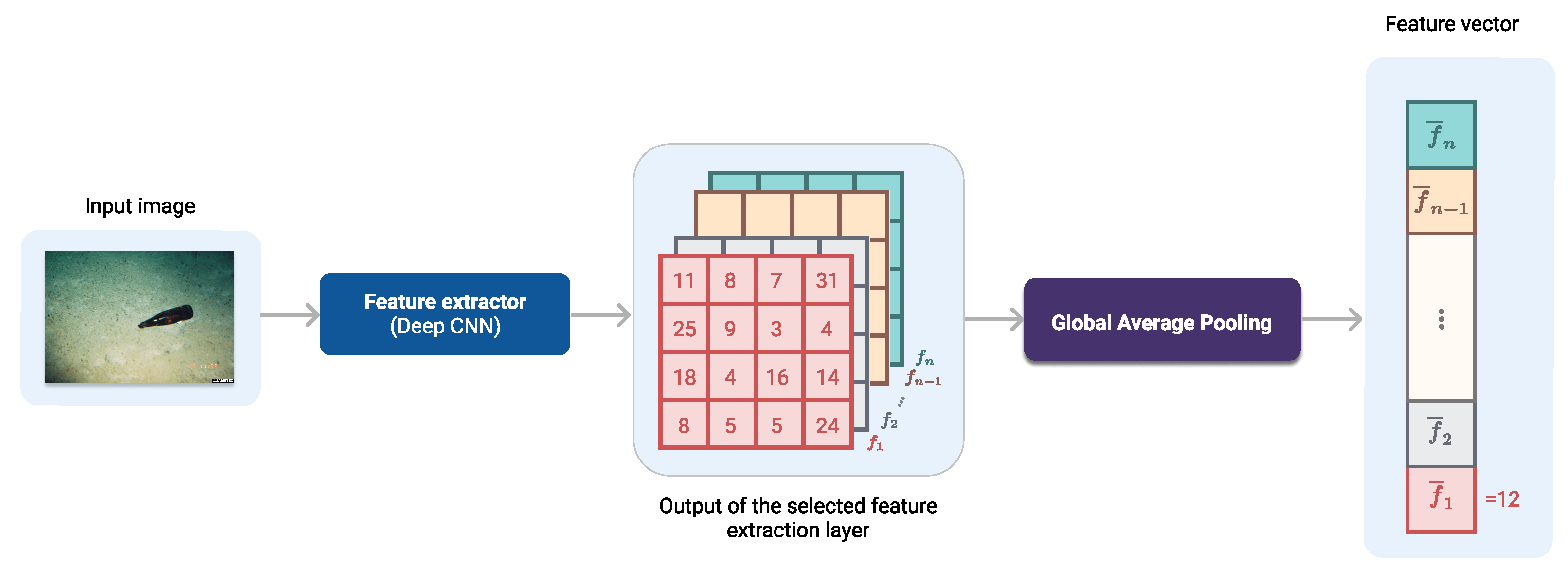
In conventional CNNs, the feature maps from the last convolutional layer are flattened into a feature vector and forwarded to fully connected layers and final softmax classification layer [21,22]. Lin et al. [62] offer an alternative with global average pooling layers, which spatially compresses the information contained in feature maps into one vector. Dense feature vectors for marine debris images are extracted using the state-of-the-art convolutional model architectures described in Section 2.2, as illustrated in Figure 15. For each model, the last layer with three-dimensional output is selected as the feature extraction layer. Global average pooling is applied to the output of that layer to obtain a feature vector from a three-dimensional output volume. Let $w\times h\times n$ be the shape of the feature extraction layer’s output and let $f_1,f_2,\dots ,f_n$ denote n feature maps in the output volume. By applying a global average pooling on the given volume, we obtain a vector $({\overline{f}}_1,{\overline{f}}_2,\dots ,{\overline{f}}_n)$ where ${\overline{f}}_i$, represents the mean value of $w·h$ values in the feature map $f_i$, $i=1,\dots ,n$. Thus, the size of the feature vector matches the depth of the output volume of the feature extraction layer.

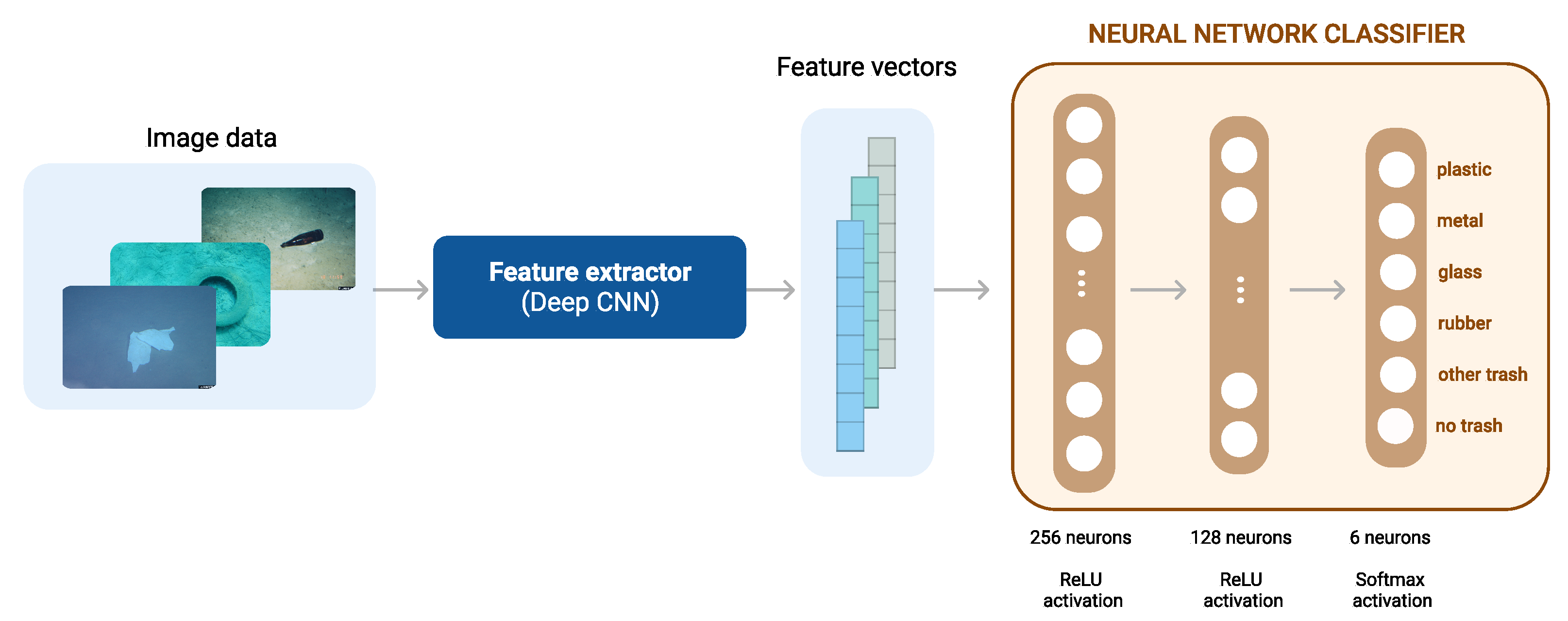
All deep models used for feature extraction are loaded with weights pre-trained on the ImageNet [34] dataset. In each deep CNN architecture, all layers that follow the feature extraction layer are dropped and replaced by a global average pooling for feature extraction.

Table 2. Deep CNN feature extractors.

Model	Input Shape	Total Parameters	Feature Vector Size
VGG19 [22]	$(224,224,3)$	20.02 M	512
InceptionV3 [51]	$(299,299,3)$	21.80 M	2048
ResNet50 [52]	$(224,224,3)$	23.59 M	2048
Inception-ResNetV2 [53]	$(299,299,3)$	54.34 M	1536
DenseNet121 [56]	$(224,224,3)$	7.04 M	1024
MobileNetV2 [56]	$(224,224,3)$	2.26 M	1280

lists all deep architectures employed in this work for feature extraction together with the information about the total number of their parameters (after dropping the layers following the feature extraction layer) and extracted vectors’ size. A new neural network (NN) classifier, which has two fully connected (FC) layers with 256 and 128 neurons followed by the Softmax layer with six neurons, is then added on top of the pooling layer, as illustrated in Figure 16. The batch normalization [63] technique is applied on newly added FC layers.

In this paper, we use deep CNN feature extractor in three different ways: (1) we freeze all its layers and train only the newly added NN classifier; (2) we fine-tune all weights of the deep CNN and train it together with the NN classifier, i.e., we use loaded Image-Net weights as the starting point for the training of the model; (3) first, we freeze deep CNN and train the NN classifier on top, and afterward unfreeze the weights of deep CNN to fine-tune them. In following sections, latter cases are denoted as (1) fixed feature extractor (FFE); (2) fine-tuning (FT); (3) FFE+FT. For the training of all models, we use Adam [64] optimizer with learning rates as in

Table 3. Learning rates.

Model	Fixed Feature Extractor	Fine-Tuning
VGG19	$5\times {10}^{-4}$	$1\times {10}^{-5}$
InceptionV3	$5\times {10}^{-4}$	$5\times {10}^{-5}$
ResNet50	$1\times {10}^{-4}$	$5\times {10}^{-5}$
Inception-ResNetV2	$1\times {10}^{-3}$	$5\times {10}^{-5}$
DenseNet121	$5\times {10}^{-4}$	$1\times {10}^{-4}$
MobileNetV2	$5\times {10}^{-4}$	$1\times {10}^{-4}$

, ${\beta }_1=0.9$, ${\beta }_2=0.999$ and $ϵ={10}^{-7}$. The learning rate of each model is chosen from the set of predefined values on a logarithmic scale using the 5-fold cross-validation.

All models were trained for 100 epochs. In the FFE+FT case, for the first 25 epochs, we train only the NN classifier on top and keep the layers of the deep CNN frozen. In the remaining 75 epochs, we fine-tune the weights of the deep CNN together with the NN classifier. For all models, we used small mini-batches of size 16, which require a smaller memory footprint than larger ones. Moreover, small batch sizes provide better generalization performance and optimization convergence [65,66]. Since we have a limited amount of data for the training at hand, we use data augmentation to expand the training set artificially. During the training, we augment images using random rotations, width and height shifts, shearing, and horizontal flipping.

For each model architecture, images are processed in an adequate format by utilizing the corresponding preprocess_input function from the tf.keras.applications (https://www.tensorflow.org/api_docs/python/tf/keras/applications, accessed on 10 June 2021) module. More precisely, for VGG19 and ResNet50 models, the images are converted from RGB to BGR image format, and each color channel is zero-centered with respect to the unscaled ImageNet data. Pixel values of input images are scaled between −1 and 1 for the InceptionV3, Inception-ResNetV2, and MobileNetV2 architectures. Finally, for the DenseNet121 architecture, pixel values are scaled between 0 and 1, and then each color channel is normalized with respect to the ImageNet data.

3.3. Simple Neural Network Architecture

To compare the performance of common pre-trained deep model architectures with the performance of smaller neural networks, we constructed a simple neural network with architecture as described in

Table 4. Simple neural network model architecture with $\approx 855K$ trainable parameters.

Layer	Kernel Size	Filters	Stride	Input Size
Conv	$3\times 3$	64	1	$(224,224,3)$
Conv	$3\times 3$	64	1	$(224,224,64)$
MaxPool	$3\times 3$	-	2	$(224,224,64)$
Conv	$3\times 3$	128	1	$(111,111,64)$
Conv	$3\times 3$	128	1	$(111,111,128)$
MaxPool	$3\times 3$	-	2	$(111,111,128)$
Conv	$3\times 3$	512	1	$(55,55,128)$
GlobalAvgPool	-	-	-	$(55,55,512)$
Softmax	-	-	-	$(1,512)$

. All convolutional layers are followed by batch normalization [63] and use ReLU nonlinearity. This neural network was trained from scratch on marine debris data for 150 epochs with mini-batches of size 16. We used the Adam optimization algorithm with the learning rate ${10}^{-4}$, ${\beta }_1=0.9$, ${\beta }_2=0.999$, and $ϵ={10}^{-7}$. Image pixel values are scaled between 0 and 1. During the training, the same augmentation techniques were used as with the pre-trained model to enlarge the training dataset artificially.

3.4. Evaluation Metrics

To evaluate the performance of marine debris classifiers, we use four quantitative metrics commonly used for multiclass classification problems: accuracy, precision, recall, and F1-score [67].

Suppose a given data set $\mathcal{D}$ contains $K>2$ different classes encoded with numbers $1,2,\dots ,K$. Let $C_{i,j}$ denote the number samples classified as class j, which actually belong to class i. The $K\times K$ matrix $C=\left[C_{i,j}\right]$ is known as the confusion matrix. The overall accuracy of a model gives the proportion of correctly classified data points and it is calculated as

$$Accuracy=\frac{{\displaystyle \sum _{i=1}^K}{C}_{i,i}}{n},$$

(3)

where n denotes the cardinality of $\mathcal{D}$. Since accuracy weighs more highly populated classes and thus strong errors on classes with just a few examples are hard to identify, we complement accuracy scores with precision, recall, and F1 metrics scores.

We introduce the following notation:

• $T{P}^{\left(i\right)}$ (True Positive): number of correctly classified instances of class i, i.e., $C_{i,i}$;
• $F{P}^{\left(i\right)}$ (False Positive): number of instances falsely classified as class i, $F{P}^{\left(i\right)}={\displaystyle \sum _{\begin{array}{c}j=1\\ j\ne i\end{array}}^K}{C}_{j,i}$;
• $F{N}^{\left(i\right)}$ (False Negative): number of instances classified as $j\ne i$ actually belonging to class i, $F{N}^{\left(i\right)}={\displaystyle \sum _{\begin{array}{c}j=1\\ j\ne i\end{array}}^K}{C}_{i,j}$.

Precision corresponding to the class i is calculated as

$$Precisio{n}^{\left(i\right)}=\frac{T{P}^{\left(i\right)}}{T{P}^{\left(i\right)}+F{P}^{\left(i\right)}},$$

(4)

while corresponding recall is given by

$$Recal{l}^{\left(i\right)}=\frac{T{P}^{\left(i\right)}}{T{P}^{\left(i\right)}+F{N}^{\left(i\right)}}.$$

(5)

Precision measures the ability of a model to return only relevant instances, while recall expresses the model’s ability to find all relevant instances in a dataset. F1-Score of the i-th class combines corresponding precision and recall scores by calculating their harmonic mean resulting in

$$F1-scor{e}^{\left(i\right)}=\frac{2Precisio{n}^{\left(i\right)}Recal{l}^{\left(i\right)}}{Precisio{n}^{\left(i\right)}+Recal{l}^{\left(i\right)}}.$$

(6)

Obtained per class metrics are aggregated in overall macro scores computed as simple arithmetic means in the following way

$$Scor{e}^{\left(macro\right)}=\frac{1}{K}\sum _{i=1}^{K}Scor{e}^{\left(i\right)},$$

(7)

where $Score$ is either $Precision$, $Recall$, or $F1-score$. Sometimes $F1-scor{e}^{\left(macro\right)}$ is calculated as $F1-scor{e}^{\left(macro2\right)}=\frac{2Precisio{n}^{\left(macro\right)}Recal{l}^{\left(macro\right)}}{Precisio{n}^{\left(macro\right)}+Recal{l}^{\left(macro\right)}}$ [67,68]. However, we use $F1-scor{e}^{\left(macro\right)}$ rather than $F1-scor{e}^{\left(macro2\right)}$, since it is more robust toward the error type distribution [68] and it is also implemented in Python’s sklearn library [61]. Macro scores do not take the class imbalance into account. Additionally, weighted scores are computed to address the uneven data distribution. Weighted scores find the average of class-wise scores weighted by the number of class instances as follows:

$$Scor{e}^{\left(weighted\right)}=\frac{1}{n}\sum _{i=1}^K{n}_{i}Scor{e}^{\left(i\right)},$$

(8)

where $n_i$ denotes the support for class i.

In addition to previously mentioned performance measures, we use Cohen’s Kappa coefficient [69], which expresses the level of agreement between classifier predictions and actual class labels. It is defined as

$$\kappa =\frac{p_o-p_e}{1-p_e},$$

(9)

where $p_o$ denotes the observational probability of agreement and $p_c$ probability of agreement by chance. $\kappa <0$ indicates poor agreement, $\kappa \in \langle 0,0.2]$ slight, $\kappa \in \langle 0.2,0.4]$ fair, $\kappa \in \langle 0.4,0.6]$ moderate, $\kappa \in \langle 0.6,0.8]$ substantial, and $\kappa \in \langle 0.8,1]$ almost perfect agreement [70]. The Kappa coefficient shows how much better the given classifier performs than the random classifier that predicts class labels based on the class frequencies.

4. Results

4.1. Deep CNN Architectures

This section compares the final performance of marine debris classifiers when different deep CNN architectures are utilized to extract image features. For each architecture, three feature extraction-tuning schemes are employed and afterward compared.

Table 5. Evaluation of NN classifiers on the test set. Since the value of the weighted recall is equal to the value of accuracy, we present only macro recall values.

Model	Scheme	Accuracy (%)	Precision (%)		Recall (%)	F1-Score (%)		Kappa
			Macro	Weighted	Macro	Macro	Weighted
	FFE	77.15	80.22	77.87	77.23	78.15	76.87	0.71
VGG19	FT	85.74	85.79	85.89	83.94	84.62	85.64	0.82
	FFE + FT	86.16	86.55	86.16	85.80	86.15	86.13	0.83
	FFE	81.34	82.62	82.14	81.45	81.75	81.46	0.77
InceptionV3	FT	90.57	90.82	90.54	91.39	91.07	90.53	0.88
	FFE + FT	89.94	91.14	90.12	89.46	90.13	89.91	0.87
	FFE	79.04	82.15	79.68	79.07	80.15	79.02	0.74
ResNet50	FT	85.12	86.60	85.34	83.51	84.65	85.02	0.81
	FFE + FT	85.53	86.31	85.59	86.82	86.51	85.51	0.82
	FFE	81.97	84.63	82.44	81.02	82.54	81.99	0.77
Inception-ResNetV2	FT	91.40	91.91	91.40	92.32	92.08	91.38	0.89
	FFE + FT	90.78	91.97	90.81	91.20	91.46	90.66	0.88
	FFE	83.02	85.07	83.72	83.81	84.19	83.14	0.79
DenseNet121	FT	88.05	89.19	88.29	87.61	88.26	88.03	0.85
	FFE + FT	87.21	87.90	87.38	86.54	87.05	87.16	0.84
	FFE	79.04	79.83	78.99	77.91	78.56	78.76	0.74
MobileNetV2	FT	82.60	83.57	82.65	82.13	82.61	82.49	0.78
	FFE + FT	81.76	81.55	82.32	79.84	80.52	81.87	0.77

shows the values of quantitative metrics described in Section 3.4 computed on the test data that were not used for the network’s training.

The overall best performance was the fine-tuned Inception-ResNetV2 model architecture, which obtained the best results of all considered metrics, including 91.40% accuracy, 92.08% (macro) F1-score, and Kappa coefficient 0.89, while fine-tuned InceptionV3 network achieves the second-best result with 90.57% accuracy, 91.07% F1-score, and Kappa coefficient of 0.88. All deep feature extraction CNNs show better performance when their weights are in some way fine-tuned, either during the whole training process or only during the second phase of the training. The overall worst performance was the VGG19 network used as a fixed feature extractor with 77.15% accuracy, 78.15% F1-score, and 0.71 Kappa coefficient, while the lightweight MobileNetV2 architecture displayed the worst performance among the fine-tuned models. Compared to the simple neural network trained from scratch (with architecture as in Table 4), which achieves the accuracy of $46.96\%$ and (macro) average precision $45.74\%$, recall $43.07\%$, and F1-score $43.68\%$, models that apply transfer learning show significantly better classification performance on test images of marine debris. A neural network trained from scratch suffers from severe overfitting; it shows good performance on the training data but has low generalization capability.

Statistician Francis Anscombe demonstrated the importance of complementing numerical calculations with data visualizations for better perception of hidden data properties not captured by statistical analyses [71]. To illustrate high-dimensional features extracted with deep CNN architectures, we use the t-SNE [72] algorithm to project feature vectors into a visualizable two-dimensional space. Figure 17 shows two-dimensional t-SNE training feature projections for best-performing Inception-ResNetV2 and lightweight MobileNetV2 architecture when three different schemes of transfer learning are used. There is a notable difference in the class-wise separation of two-dimensional features when the model fine-tunes the pre-trained weights on the task of interest and when a deep feature extractor stays fixed. During the fine-tuning, a deep CNN extractor adjusts its weights so that new features incorporate details and peculiarities of marine images important for the characterization of each of the six considered classes. Thus, the fine-tuned features better discriminate between these classes. Greater separation between semantic clusters of features can be seen in the better-performing FT Inception model (Figure 17).

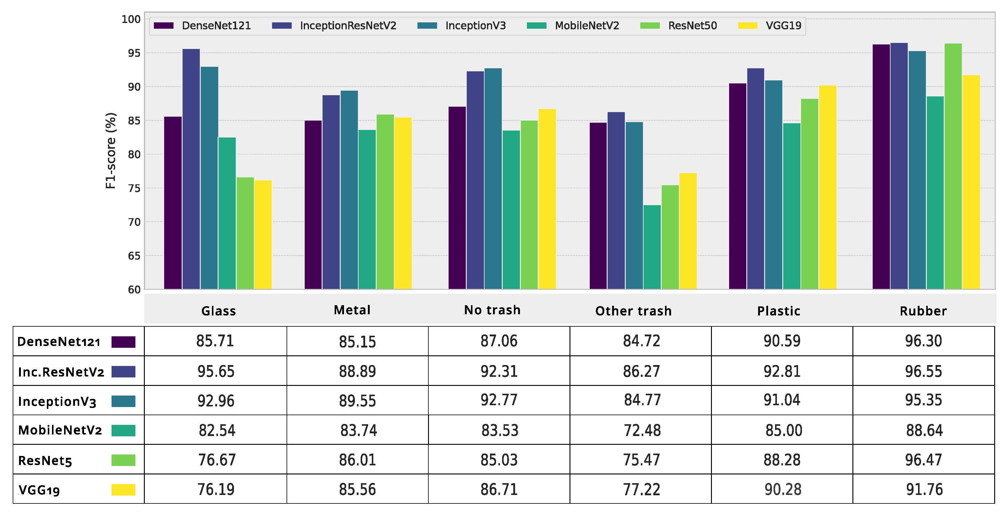
In general, models obtain higher precision than recall, i.e., fewer false positives than false negatives per class. Figure 18 shows class-wise F1-scores for each deep CNN architecture. The weakest performance is observed on the Other garbage class with high in-class variations and the best in the Rubber class due to the unique round shape of class objects and lower range of in-class variations. Aside from the low performance in the Other Trash class, models that used the ResNet50 and VGG19 extractors did not show the best performance in the Glass class either.

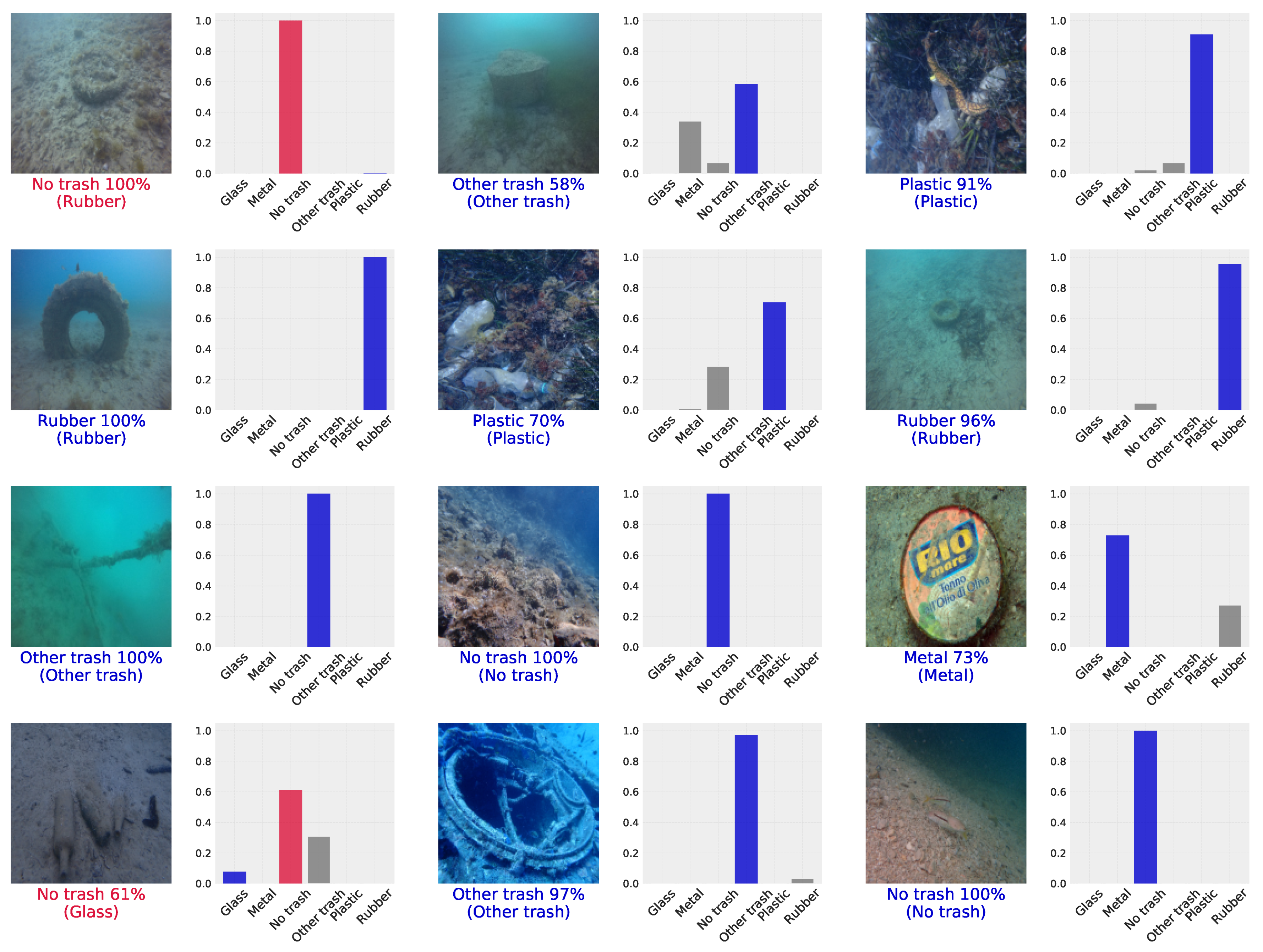
Figure 19 shows predictions of the FT Inception model on new images of waste items collected by local divers in the Croatian Adriatic sea, more precisely, in the bays in the area Split and the island of Korčula. These local images were not used during the training nor testing. They are the first step toward creating a new local dataset for marine debris classification and identification in Adriatic Sea underwaters. The network trained on deep-sea images shows promising results in a new aquatic environment with different sea transparency and salinity, seabed sediments, and unique flora and fauna.

4.2. Deep Feature Classification with Conventional ML Classifiers

The neural network classifier on top of the deep feature extractor can be replaced with any conventional ML classifier.

Table 6. Performance of machine learning classifiers on the test set.

Model	Classifier	Accuracy (%)	F1-Score (%)	Kappa
VGG19 (FFE + FT)	NN	86.16	86.15	0.83
	RF	80.08	78.84	0.75
	SVM	84.28	83.57	0.80
	NB	68.97	67.04	0.61
	LR	80.71	79.95	0.76
	KNN	73.79	72.53	0.67
InceptionV3 (FT)	NN	90.57	91.07	0.88
	RF	88.47	88.42	0.86
	SVM	90.57	90.89	0.88
	NB	88.47	88.60	0.86
	LR	90.78	91.28	0.88
	KNN	89.52	90.13	0.87
ResNet50 (FFE + FT)	NN	85.53	86.51	0.82
	RF	83.02	82.83	0.79
	SVM	86.16	87.07	0.83
	NB	81.55	82.03	0.77
	LR	85.95	86.97	0.82
	KNN	79.66	79.47	0.74
Inception-ResNetV2 (FT)	NN	91.40	92.08	0.89
	RF	90.99	91.80	0.89
	SVM	91.61	92.27	0.90
	NB	90.99	91.75	0.89
	LR	90.99	91.60	0.89
	KNN	90.15	90.94	0.88
DenseNet121 (FT)	NN	88.05	88.26	0.85
	RF	85.74	85.52	0.82
	SVM	88.05	88.53	0.85
	NB	83.02	83.52	0.79
	LR	86.79	86.58	0.83
	KNN	84.28	84.91	0.80
MobileNetV2 (FT)	NN	82.60	82.61	0.78
	RF	84.07	83.56	0.80
	SVM	85.32	85.62	0.82
	NB	84.49	84.40	0.81
	LR	83.02	83.47	0.79
	KNN	82.39	83.14	0.78

provides the classification results of RF, SVM, NB, LR, and KNN classifier trained on deep features extracted with the best performing feature extraction scheme (see Table 5) for a given CNN architecture. As we can see from Table 6, by replacing the NN classifier by SVM or LR classifier, the performance on new data in many cases improves, e.g., SVM classifier with Inception-ResNetV2 obtains 91.61% accuracy, 92.27% macro F1-score, and 0.90 Kappa coefficient, as opposed to 91.40% accuracy, 92.08% F1-score, and 0.89 Kappa of the NN classifier. The most significant improvement was observed with the MobileNetV2 feature extractor, which obtains the best classification result with an SVM of accuracy 85.32% compared to 82.60% accuracy of the NN classifier.

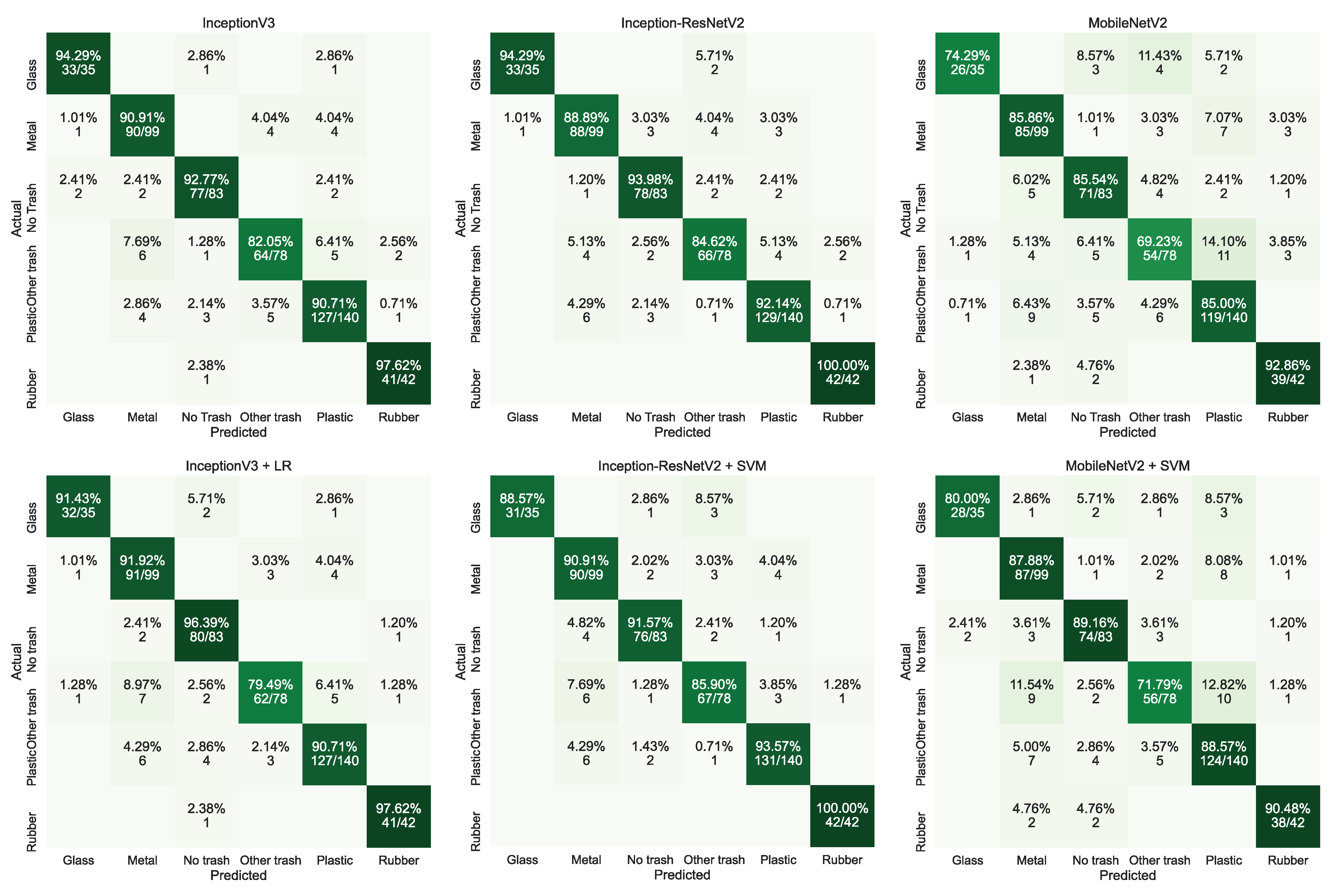
Figure 20 shows the confusion matrices for the best-performing Inception architectures (InceptionV3 and Inception-ResNetV2) and a lightweight MobileNetV2 architecture designed to meet the resource constraints of mobile and embedded devices. Although replacing the NN classifier by an ML classifier did result in a slight boost of model’s overall performance on new data, in several cases the performance on some classes dropped, e.g., Other trash for InceptionV3 and No trash for the Inception-ResNetV2. The confusion across all models (in NN and ML classifiers) is the most pronounced at the Other trash class with corresponding images often assigned to classes Metal and Plastic, and vice versa. Furthermore, misconceptions of plastic as metal and metal as plastic often occur. The confusion of No trash images with different categories of marine litter can be attributed to the various non-waste objects found in such images, such as other marine life objects, seagrass, and rocks.

5. Discussion

This study analyzes the performance of well-known deep CNN architectures when utilized as feature extractors to classify underwater images of marine debris with neural networks and other conventional ML classifiers. Fine-tuned deep CNN feature extractors that stack Inception modules, Inception-ResNetV2 and InceptionV3, show the overall best performance in our experimental setup (see Table 5 and Table 6). With increasing depth, these architectures simultaneously increase the width of the network by introducing parallel convolutions. Although MobileNetV2 architecture’s performance is ranked as the worst, it should not be written off easily since this architecture comes with several advantages desirable for implementation in embedded devices: faster performance, reduced network size, and low latency. With the choice of MobileNetV2 architecture for feature extraction, one sacrifices overall accuracy for computational efficiency.

Several works have employed deep-learning-based approaches to marine debris detection and classification in underwater imagery in recent years.

Table 7. Comparison of the performance of different approaches to the detection and classification of marine debris presented in the literature.

Dataset	Classes	Network	Problem	Reported Result
J-EDI dataset (Fulton et al. [27])	3 classes: Plastic, ROV, Bio	YOLOv2 FT	object detection	maAP = 47.9
		Tiny-YOLO	object detection	mAP = 31.6
		Faster RCNN (with InceptionV2)	object detection	mAP = 81.0
		SSD MultiBox (with MobileNetV2)	object detection	mAP = 67.4
ARIS Explorerx 3000 FLS household marine debris dataset (Valdenegro-Toro [23])	6 classes: Metal, Glass, Cardboard, Rubber, Plastic, Background	CNN (four layers)	classification	accuracy = 97.1
			object detection	correct detect. = 70.8
Underwater Sea Litter dataset natural and synthetic data (Musić et al. [29])	5 classes: Cardboard, Glass, Paper, Metal, Plastic	VGG16	classification	accuracy = 85.0
		custom CNN	classification	accuracy = 81.5
		YOLOv3 (threshold 0.75)	object detection	recall = 43.0 precision = 71.0 accuracy = 36.0
LIFE DEBAG Seafloor Marine Litter dataset (Politikos et al. [28])	11 classes: pl. bags, pl. bottles, pl. sheets, pl. cups, tires, big object, pl. caps, small pl. sheets, cans, fishing nets, unspecified	Mask R-CNN (IoU threshold 25%)	object detection	mAP = 66.0
		Mask R-CNN (IoU threshold 50%)	object detection	mAP = 62.0
		Mask R-CNN (IoU threshold 75%)	object detection	maP = 45.0

gives an overview of results presented in the literature using different network architectures. While [27,28,29] use realistic underwater images, Ref. [23] uses forward-looking sonar (FLS) imagery with constructed $96\times 96$ image crops of debris objects utilized for classifier’s training and testing. In terms of accuracy, classifcation model from [23] gives better results than similar models trained and validated on underwater RGB images that do not contain only one centered debris object, as expected. In contrast to studies presented in Table 7, our work compares the performance of six well-known CNN architectures (VGG19, InceptionV3, ResNet50, Inception-ResNetV2, DenseNetV2, and MobileNetV2) combined with NN, RF, SVM, NB, LR, and KNN classifiers. The best reported result with an accuracy of $91.61\%$ is obtained with fine-tuned Inception-ResNetV2 feature extractor and SVM classifier. Despite the intrinsic challenges of the used dataset, with the choice of appropriate feature-extractor network architectures, the scheme for its deployment, and the appropriate classifier, satisfactory results on new images are obtained.

This paper focuses exclusively on image classification based on deep learning feature extraction. Alternatively, traditional computer vision techniques can be used for feature extraction from raw pixel data. The problem with traditional approach is that it requires careful fine-tuning and expert analysis. This is especially evident in multiclass classification problems. Each class requires manual feature engineering in order to describe best its typical object patterns, which becomes a real burden with many parameters to tweak [49]. On the other hand, DL methods mitigate the need for manual extraction of features and provide the end-to-end learning process, which extracts relevant image features automatically and often outperforms conventional feature extraction techniques [73,74].

Traditional “crisp” algorithms for image classification do not fully consider inherent uncertainties and peculiarities present in debris images from the realistic underwater environment. Image entities belonging to the same debris class often significantly vary in shape and entity position. Moreover, images are often affected by uncertainties such as current recording angle, water turbidity, and illumination, implying the inherent fuzzy nature of the given dataset. In order to address this problem, specific classifiers based on fuzzy techniques can be applied. The success of the fuzzy approach to classification and clustering has been reported on datasets with inherent uncertainties from various domains [75,76,77]. Based on these findings, it would be interesting to investigate further whether the fuzzy-based techniques can enhance the classification performance on the use-case of marine debris identification and classification. However, this falls out of the scope of this paper and is planned for future research.

6. Conclusions

Marine debris poses a major threat to the marine ecosystem and negatively affects today’s society in an environmental, social, and economical way. Motivated by the need for automatic and cost-effective approaches for marine debris monitoring and removal, we employ machine learning techniques together with deep learning-based feature extraction to identify and classify marine debris in a realistic underwater environment. This paper provides a comparative analysis of common deep convolutional architectures used as feature extractors for underwater image classification. Furthermore, it explores the best ways to use deep feature extractors by analyzing three different modes for utilizing pre-trained deep feature extractors and examining the performance of different ML-based classifiers trained on top of extracted features.

The fine-tuning of the pre-trained feature extractor network’s weights with appropriate learning rates during the whole training procedure showed the most prominent results in our experimental setup. The best performance is shown by Inception-based FT feature extractors, namely Inception-ResNetV2 and InceptionV3, achieving an overall accuracy of more than 90%, more precisely 91.40%, and 90.57%, respectively, when trained with the NN classifier on top. Traditional SVM and LR classifiers exhibited as credible alternatives to the NN classifier, which often outperform the NN classifier. The SVM trained on Inception-ResNetV2 features achieves 91.61% accuracy, while the LR classifier trained on the InceptionV3 features obtains accuracy of 90.78%. Considering the inherent challenges that come with automatic marine debris classification in underwater imagery, the obtained results demonstrate the potential for further exploitation of deep-learning-based models for real-time marine debris identification and classification in natural aquatic environments.

In the future, we hope to assemble our dataset containing images of marine debris in Croatian Adriatic Sea underwaters to utilize a deep-learning approach for automatic marine debris identification in the local marine environment. The main focus of this paper is the problem of marine debris classification. Future research should focus on expanding the conducted analysis to detect waste objects under the sea level: comparing different object detection architectures with different backbone convolutional network architectures. Furthermore, this work discusses only three approaches to transfer learning: (1) keeping the pre-trained feature extractor network frozen; (2) fine-tuning its weights during the whole training procedure; (3) freezing the feature extractor during the first phase of training and afterward unfreezing it to fine-tune its weights during the second training phase. In future research, it would be interesting to extend the analysis to the case where the first layers of the pre-trained feature extractor network remain fixed while the rest of the network corresponding to more domain-specific features become fine-tuned. Moreover, the optimal way to split the feature extractor into a frozen and fine-tuned part can be further analyzed for each network architecture.

References

1. Sheavly, S.; Register, K. Marine debris & plastics: Environmental concerns, sources, impacts and solutions. J. Polym. Environ. 2007, 15, 301–305. [Google Scholar] [CrossRef]
2. Savoca, M.S.; Wohlfeil, M.E.; Ebeler, S.E.; Nevitt, G.A. Marine plastic debris emits a keystone infochemical for olfactory foraging seabirds. Sci. Adv. 2016, 2, e1600395. [Google Scholar] [CrossRef] [Green Version]
3. Pfaller, J.B.; Goforth, K.M.; Gil, M.A.; Savoca, M.S.; Lohmann, K.J. Odors from marine plastic debris elicit foraging behavior in sea turtles. Curr. Biol. 2020, 30, R213–R214. [Google Scholar] [CrossRef]
4. Lusher, A.; Hollman, P.; Mendoza-Hill, J. Microplastics in Fisheries and Aquaculture: Status of Knowledge on Their Occurrence and Implications for Aquatic Organisms and Food Safety; FAO: Rome, Italy, 2017. [Google Scholar]
5. Smith, M.; Love, D.C.; Rochman, C.M.; Neff, R.A. Microplastics in seafood and the implications for human health. Curr. Environ. Health Rep. 2018, 5, 375–386. [Google Scholar] [CrossRef] [Green Version]
6. Meeker, J.D.; Sathyanarayana, S.; Swan, S.H. Phthalates and other additives in plastics: Human exposure and associated health outcomes. Philos. Trans. R. Soc. B: Biol. Sci. 2009, 364, 2097–2113. [Google Scholar] [CrossRef] [Green Version]
7. Newman, S.; Watkins, E.; Farmer, A.; Ten Brink, P.; Schweitzer, J.P. The economics of marine litter. In Marine Anthropogenic Litter; Springer: Cham, The Netherlands, 2015; pp. 367–394. [Google Scholar] [CrossRef] [Green Version]
8. Williams, A.; Rangel-Buitrago, N. Marine Litter: Solutions for a Major Environmental Problem. J. Coast. Res. 2019, 35, 648–663. [Google Scholar] [CrossRef] [Green Version]
9. Ren, S.; He, K.; Girshick, R.; Sun, J. Faster r-cnn: Towards real-time object detection with region proposal networks. arXiv 2015, arXiv:1506.01497. [Google Scholar] [CrossRef] [Green Version]
10. Bochkovskiy, A.; Wang, C.Y.; Liao, H.Y.M. Yolov4: Optimal speed and accuracy of object detection. arXiv 2020, arXiv:2004.10934. [Google Scholar]
11. Tan, M.; Le, Q. Efficientnet: Rethinking model scaling for convolutional neural networks. In Proceedings of the International Conference on Machine Learning (ICML), Long Beach, CA, USA, 10–15 June 2019; pp. 6105–6114. [Google Scholar]
12. Brock, A.; De, S.; Smith, S.L.; Simonyan, K. High-Performance Large-Scale Image Recognition Without Normalization. arXiv 2021, arXiv:2102.06171. [Google Scholar]
13. Tao, A.; Sapra, K.; Catanzaro, B. Hierarchical multi-scale attention for semantic segmentation. arXiv 2020, arXiv:2005.10821. [Google Scholar]
14. Zhu, Y.; Sapra, K.; Reda, F.A.; Shih, K.J.; Newsam, S.; Tao, A.; Catanzaro, B. Improving semantic segmentation via video propagation and label relaxation. In Proceedings of the IEEE/CVF Conference on Computer Vision and Pattern Recognition, Long Beach, CA, USA, 16–20 June 2019; pp. 8856–8865. [Google Scholar]
15. LeCun, Y.; Bengio, Y.; Hinton, G. Deep learning. Nature 2015, 521, 436–444. [Google Scholar] [CrossRef]
16. LeCun, Y.; Boser, B.; Denker, J.S.; Henderson, D.; Howard, R.E.; Hubbard, W.; Jackel, L.D. Backpropagation applied to handwritten zip code recognition. Neural Comput. 1989, 1, 541–551. [Google Scholar] [CrossRef]
17. Hubel, D.H.; Wiesel, T.N. Receptive fields and functional architecture of monkey striate cortex. J. Physiol. 1968, 195, 215–243. [Google Scholar] [CrossRef]
18. Fukushima, K. Neocognitron. Scholarpedia 2007, 2, 1717. [Google Scholar] [CrossRef]
19. Nair, V.; Hinton, G.E. Rectified Linear units Improve Restricted Boltzmann Machines. In Proceedings of the 27th International Conference on Machine Learning (ICML-10), Haifa, Israel, 21–24 June 2010; pp. 807–814. [Google Scholar]
20. Gu, J.; Wang, Z.; Kuen, J.; Ma, L.; Shahroudy, A.; Shuai, B.; Liu, T.; Wang, X.; Wang, G.; Cai, J.; et al. Recent advances in convolutional neural networks. Pattern Recognit. 2018, 77, 354–377. [Google Scholar] [CrossRef] [Green Version]
21. Krizhevsky, A.; Sutskever, I.; Hinton, G.E. Imagenet classification with deep convolutional neural networks. Adv. Neural Inf. Process. Syst. 2012, 25, 1097–1105. [Google Scholar] [CrossRef]
22. Simonyan, K.; Zisserman, A. Very deep convolutional networks for large-scale image recognition. arXiv 2014, arXiv:1409.1556. [Google Scholar]
23. Valdenegro-Toro, M. Submerged marine debris detection with autonomous underwater vehicles. In Proceedings of the 2016 International Conference on Robotics and Automation for Humanitarian Applications (RAHA), Amritapuri, India, 18–20 December 2016; pp. 1–7. [Google Scholar]
24. Panwar, H.; Gupta, P.; Siddiqui, M.K.; Morales-Menendez, R.; Bhardwaj, P.; Sharma, S.; Sarker, I.H. AquaVision: Automating the detection of waste in water bodies using deep transfer learning. Case Stud. Chem. Environ. Eng. 2020, 2, 100026. [Google Scholar] [CrossRef]
25. Kylili, K.; Kyriakides, I.; Artusi, A.; Hadjistassou, C. Identifying floating plastic marine debris using a deep learning approach. Environ. Sci. Pollut. Res. 2019, 26, 17091–17099. [Google Scholar] [CrossRef]
26. Kylili, K.; Hadjistassou, C.; Artusi, A. An intelligent way for discerning plastics at the shorelines and the seas. Environ. Sci. Pollut. Res. 2020, 27, 42631–42643. [Google Scholar] [CrossRef]
27. Fulton, M.; Hong, J.; Islam, M.J.; Sattar, J. Robotic detection of marine litter using deep visual detection models. In Proceedings of the 2019 International Conference on Robotics and Automation (ICRA), Montreal, QC, Canada, 20–24 May 2019; pp. 5752–5758. [Google Scholar] [CrossRef] [Green Version]
28. Politikos, D.V.; Fakiris, E.; Davvetas, A.; Klampanos, I.A.; Papatheodorou, G. Automatic detection of seafloor marine litter using towed camera images and deep learning. Mar. Pollut. Bull. 2021, 164, 111974. [Google Scholar] [CrossRef]
29. Musić, J.; Kružić, S.; Stančić, I.; Alexandrou, F. Detecting Underwater Sea Litter Using Deep Neural Networks: An Initial Study. In Proceedings of the 2020 5th International Conference on Smart and Sustainable Technologies (SpliTech), Split, Croatia, 23–26 September 2020; pp. 1–6. [Google Scholar] [CrossRef]
30. Lorenzo-Navarro, J.; Castrillón-Santana, M.; Santesarti, E.; De Marsico, M.; Martínez, I.; Raymond, E.; Gómez, M.; Herrera, A. SMACC: A System for Microplastics Automatic Counting and Classification. IEEE Access 2020, 8, 25249–25261. [Google Scholar] [CrossRef]
31. Fallati, L.; Polidori, A.; Salvatore, C.; Saponari, L.; Savini, A.; Galli, P. Anthropogenic Marine Debris assessment with Unmanned Aerial Vehicle imagery and deep learning: A case study along the beaches of the Republic of Maldives. Sci. Total Environ. 2019, 693, 133581. [Google Scholar] [CrossRef] [PubMed]
32. Kako, S.; Morita, S.; Taneda, T. Estimation of plastic marine debris volumes on beaches using unmanned aerial vehicles and image processing based on deep learning. Mar. Pollut. Bull. 2020, 155, 111127. [Google Scholar] [CrossRef] [PubMed]
33. Pan, S.J.; Yang, Q. A Survey on Transfer Learning. IEEE Trans. Knowl. Data Eng. 2010, 22, 1345–1359. [Google Scholar] [CrossRef]
34. Deng, J.; Dong, W.; Socher, R.; Li, L.J.; Li, K.; Fei-Fei, L. ImageNet: A Large-Scale Hierarchical Image Database. CVPR09, 2009. Available online: http://www.image-net.org/ (accessed on 2 May 2021).
35. Sharif Razavian, A.; Azizpour, H.; Sullivan, J.; Carlsson, S. CNN features off-the-shelf: An astounding baseline for recognition. In Proceedings of the IEEE Conference on Computer Vision and Pattern Recognition Workshops, Columbus, OH, USA, 23–28 June 2014; pp. 806–813. [Google Scholar] [CrossRef] [Green Version]
36. Donahue, J.; Jia, Y.; Vinyals, O.; Hoffman, J.; Zhang, N.; Tzeng, E.; Darrell, T. Decaf: A deep convolutional activation feature for generic visual recognition. In Proceedings of the International Conference on Machine Learning, PMLR, Bejing, China, 22–24 June 2014; pp. 647–655. [Google Scholar]
37. Yosinski, J.; Clune, J.; Bengio, Y.; Lipson, H. How transferable are features in deep neural networks? arXiv 2014, arXiv:1411.1792. [Google Scholar]
38. Azizpour, H.; Sharif Razavian, A.; Sullivan, J.; Maki, A.; Carlsson, S. From generic to specific deep representations for visual recognition. In Proceedings of the IEEE Conference on Computer Vision and Pattern Recognition Workshops, Boston, MA, USA, 7–12 June 2015; pp. 36–45. [Google Scholar] [CrossRef] [Green Version]
39. Ben Jabra, M.; Koubaa, A.; Benjdira, B.; Ammar, A.; Hamam, H. COVID-19 Diagnosis in Chest X-rays Using Deep Learning and Majority Voting. Appl. Sci. 2021, 11, 2884. [Google Scholar] [CrossRef]
40. Esteva, A.; Kuprel, B.; Novoa, R.A.; Ko, J.; Swetter, S.M.; Blau, H.M.; Thrun, S. Dermatologist-level classification of skin cancer with deep neural networks. Nature 2017, 542, 115–118. [Google Scholar] [CrossRef]
41. Wang, X.; Peng, Y.; Lu, L.; Lu, Z.; Bagheri, M.; Summers, R.M. ChestX-ray8: Hospital-scale chest X-ray database and benchmarks on weakly-supervised classification and localization of common thorax diseases. In Proceedings of the IEEE Conference on Computer Vision and Pattern Recognition, Honolulu, HI, USA, 21–26 July 2017; pp. 2097–2106. [Google Scholar] [CrossRef] [Green Version]
42. Karri, S.P.K.; Chakraborty, D.; Chatterjee, J. Transfer learning based classification of optical coherence tomography images with diabetic macular edema and dry age-related macular degeneration. Biomed. Opt. Express 2017, 8, 579–592. [Google Scholar] [CrossRef] [Green Version]
43. Chen, J.; Chen, J.; Zhang, D.; Sun, Y.; Nanehkaran, Y. Using deep transfer learning for image-based plant disease identification. Comput. Electron. Agric. 2020, 173, 105393. [Google Scholar] [CrossRef]
44. Qi, H.; Liang, Y.; Ding, Q.; Zou, J. Automatic Identification of Peanut-Leaf Diseases Based on Stack Ensemble. Appl. Sci. 2021, 11, 1950. [Google Scholar] [CrossRef]
45. Jeon, H.K.; Kim, S.; Edwin, J.; Yang, C.S. Sea Fog Identification from GOCI Images Using CNN Transfer Learning Models. Electronics 2020, 9, 311. [Google Scholar] [CrossRef]
46. Mahdianpari, M.; Salehi, B.; Rezaee, M.; Mohammadimanesh, F.; Zhang, Y. Very Deep Convolutional Neural Networks for Complex Land Cover Mapping Using Multispectral Remote Sensing Imagery. Remote Sens. 2018, 10, 1119. [Google Scholar] [CrossRef] [Green Version]
47. Iqbal Hussain, M.A.; Khan, B.; Wang, Z.; Ding, S. Woven Fabric Pattern Recognition and Classification Based on Deep Convolutional Neural Networks. Electronics 2020, 9, 1048. [Google Scholar] [CrossRef]
48. Japan Agency for Marine Earth Science and Technology, Deep-sea Debris Database. Available online: http://www.godac.jamstec.go.jp/catalog/dsdebris/metadataList?lang=en (accessed on 14 March 2021).
49. O’Mahony, N.; Campbell, S.; Carvalho, A.; Harapanahalli, S.; Hernandez, G.V.; Krpalkova, L.; Riordan, D.; Walsh, J. Deep Learning vs. Traditional Computer Vision. In Advances in Computer Vision; Arai, K., Kapoor, S., Eds.; Springer International Publishing: Cham, The Netherlands, 2020; pp. 128–144. [Google Scholar]
50. Szegedy, C.; Liu, W.; Jia, Y.; Sermanet, P.; Reed, S.; Anguelov, D.; Erhan, D.; Vanhoucke, V.; Rabinovich, A. Going deeper with convolutions. In Proceedings of the IEEE Conference on Computer Vision and Pattern Recognition, Boston, MA, USA, 7–12 June 2015; pp. 1–9. [Google Scholar] [CrossRef] [Green Version]
51. Szegedy, C.; Vanhoucke, V.; Ioffe, S.; Shlens, J.; Wojna, Z. Rethinking the inception architecture for computer vision. In Proceedings of the IEEE Conference on Computer Vision and Pattern Recognition, Las Vegas, NV, USA, 27–30 June 2016; pp. 2818–2826. [Google Scholar] [CrossRef] [Green Version]
52. He, K.; Zhang, X.; Ren, S.; Sun, J. Deep residual learning for image recognition. In Proceedings of the IEEE Conference on Computer Vision and Pattern Recognition, Las Vegas, NV, USA, 27–30 June 2016; pp. 770–778. [Google Scholar] [CrossRef] [Green Version]
53. Szegedy, C.; Ioffe, S.; Vanhoucke, V.; Alemi, A. Inception-v4, inception-resnet and the impact of residual connections on learning. In Proceedings of the AAAI Conference on Artificial Intelligence, San Francisco, CA, USA, 4–9 February 2017; Volume 31. [Google Scholar]
54. Huang, G.; Liu, Z.; Van Der Maaten, L.; Weinberger, K.Q. Densely connected convolutional networks. In Proceedings of the IEEE Conference on Computer Vision and Pattern Recognition, Honolulu, HI, USA, 21–26 July 2017; pp. 4700–4708. [Google Scholar] [CrossRef] [Green Version]
55. Howard, A.G.; Zhu, M.; Chen, B.; Kalenichenko, D.; Wang, W.; Weyand, T.; Andreetto, M.; Adam, H. Mobilenets: Efficient convolutional neural networks for mobile vision applications. arXiv 2017, arXiv:1704.04861. [Google Scholar]
56. Sandler, M.; Howard, A.; Zhu, M.; Zhmoginov, A.; Chen, L.C. Mobilenetv2: Inverted residuals and linear bottlenecks. In Proceedings of the IEEE Conference on Computer Vision and Pattern Recognition, Salt Lake City, UT, USA, 18–23 June 2018; pp. 4510–4520. [Google Scholar] [CrossRef] [Green Version]
57. Breiman, L. Random forests. Mach. Learn. 2001, 45, 5–32. [Google Scholar] [CrossRef] [Green Version]
58. Vapnik, V.N. The Nature of Statistical Learning Theory; Springer: New York, NY, USA, 1995. [Google Scholar] [CrossRef]
59. Abadi, M.; Agarwal, A.; Barham, P.; Brevdo, E.; Chen, Z.; Citro, C.; Corrado, G.S.; Davis, A.; Dean, J.; Devin, M.; et al. TensorFlow: Large-Scale Machine Learning on Heterogeneous Systems. 2015. Available online: https://www.tensorflow.org/ (accessed on 17 June 2021).
60. Chollet, F. Keras. 2015. Available online: https://github.com/fchollet/keras (accessed on 2 May 2021).
61. Pedregosa, F.; Varoquaux, G.; Gramfort, A.; Michel, V.; Thirion, B.; Grisel, O.; Blondel, M.; Prettenhofer, P.; Weiss, R.; Dubourg, V.; et al. Scikit-learn: Machine Learning in Python. J. Mach. Learn. Res. 2011, 12, 2825–2830. [Google Scholar]
62. Lin, M.; Chen, Q.; Yan, S. Network in network. arXiv 2013, arXiv:1312.4400. [Google Scholar]
63. Ioffe, S.; Szegedy, C. Batch Normalization: Accelerating Deep Network Training by Reducing Internal Covariate Shift. In Proceedings of the 32nd International Conference on International Conference on Machine Learning, Lille, France, 7–9 July 2015; Volume 37, pp. 448–456. [Google Scholar]
64. Kingma, D.P.; Ba, J. Adam: A method for stochastic optimization. arXiv 2014, arXiv:1412.6980. [Google Scholar]
65. Wilson, D.R.; Martinez, T.R. The general inefficiency of batch training for gradient descent learning. Neural Netw. 2003, 16, 1429–1451. [Google Scholar] [CrossRef] [Green Version]
66. Masters, D.; Luschi, C. Revisiting small batch training for deep neural networks. arXiv 2018, arXiv:1804.07612. [Google Scholar]
67. Sokolova, M.; Lapalme, G. A systematic analysis of performance measures for classification tasks. Inf. Process. Manag. 2009, 45, 427–437. [Google Scholar] [CrossRef]
68. Opitz, J.; Burst, S. Macro f1 and macro f1. arXiv 2019, arXiv:1911.03347. [Google Scholar]
69. Cohen, J. A coefficient of agreement for nominal scales. Educ. Psychol. Meas. 1960, 20, 37–46. [Google Scholar] [CrossRef]
70. Landis, J.R.; Koch, G.G. The measurement of observer agreement for categorical data. Biometrics 1977, 33, 159–174. [Google Scholar] [CrossRef] [Green Version]
71. Anscombe, F.J. Graphs in Statistical Analysis. Am. Stat. 1973, 27, 17–21. [Google Scholar]
72. Van der Maaten, L.; Hinton, G. Visualizing data using t-SNE. J. Mach. Learn. Res. 2008, 9, 2580–2605. [Google Scholar]
73. Zhu, L.; Spachos, P. Towards Image Classification with Machine Learning Methodologies for Smartphones. Mach. Learn. Knowl. Extr. 2019, 1, 59. [Google Scholar] [CrossRef] [Green Version]
74. Sykora, P.; Kamencay, P.; Hudec, R.; Benco, M.; Sinko, M. Comparison of Feature Extraction Methods and Deep Learning Framework for Depth Map Recognition. In Proceedings of the 2018 New Trends in Signal Processing (NTSP), Liptovsky Mikulas, Slovakia, 10–12 October 2018; pp. 1–7. [Google Scholar] [CrossRef]
75. Postorino, M.N.; Versaci, M. A geometric fuzzy-based approach for airport clustering. Adv. Fuzzy Syst. 2014, 2014. [Google Scholar] [CrossRef] [Green Version]
76. Mahmoudi, M.R.; Baleanu, D.; Qasem, S.N.; Mosavi, A.; Band, S.S. Fuzzy clustering to classify several time series models with fractional Brownian motion errors. Alex. Eng. J. 2021, 60, 1137–1145. [Google Scholar] [CrossRef]
77. Xu, K.; Pedrycz, W.; Li, Z.; Nie, W. Optimizing the prototypes with a novel data weighting algorithm for enhancing the classification performance of fuzzy clustering. Fuzzy Sets Syst. 2021, 413, 29–41. [Google Scholar] [CrossRef]
Figure 1. Sample of images from the dataset.
Applsci 11 05644 g001
Figure 2. VGG19 network architecture. Input to the VGG19 network is 224 × 224 RGB image. Convolutional layers are labeled as “ conv s , n ”, where s denotes the filter size and n number of filters in a given layer. All layers, besides the last Softmax layer, use the ReLU activation function. MaxPooling is applied on 2 × 2 patches with a stride of 2. The feature maps produced by the max-pooling layer in Block 5 are flattened into a single 25088-dimensional vector and fed into fully connected layers.
Applsci 11 05644 g002
Figure 3. GoogLeNet Inception module. The concatenation layer concatenates outputs x 1 , , x 4 of the four preceding convolutional layers of the shape ( w , h , d i ) , i = 1 , , 4 , into one volume x = [ x 1 , , x 4 ] of the shape ( w , h , i = 1 4 d i ) , which is forwarded to the following network’s layer.
Applsci 11 05644 g003
Figure 4. Modules of InceptionV3 architecture.
Applsci 11 05644 g004
Figure 5. InceptionV3 architecture.
Applsci 11 05644 g005
Figure 6. Two types of residual modules. Modules calculate f R ( x ) + g ( x ) (element-wise) where x denotes the module’s input, f R ( x ) the output of three stacked convolutional layers, and g the projection function used to match x and f R ( x ) dimensions in the convolution block, and the identity function g ( x ) = x in the identity block.
Applsci 11 05644 g006
Figure 7. ResNet50 architecture.
Applsci 11 05644 g007
Figure 8. Inception-ResNetV2 modules.
Applsci 11 05644 g008
Figure 9. Inception-ResNetV2 architecture.
Applsci 11 05644 g009
Figure 10. Dense connectivity. Instead of m (layer-wise) connections, m-layer densely connected network has m ( m + 1 ) 2 layer-wise connections.
Applsci 11 05644 g010
Figure 11. DenseNet121 architecture. Each "Conv" block corresponds to batch normalization + ReLU + convolution.
Applsci 11 05644 g011
Figure 12. Dense block with m building blocks.
Applsci 11 05644 g012
Figure 13. MobileNetV2 building blocks. Idea: (1) uncompress recived data (2) filter data using the lightweighted depth-wise convolution (3) compress data to low-dimensional representation (4) combine input data with new compressed data representation. Point-wise convolutional layer in MobileNetV2 architecture is also known as the projection layer since it projects data with large number of channels into smaller-depth output ( e d > > f ).
Applsci 11 05644 g013
Figure 14. MobileNetV2 architecture.
Applsci 11 05644 g014
Figure 15. Extraction of dense feature vectors.
Applsci 11 05644 g015
Figure 16. Classification of marine debris images using a neural network classifier, which receives extracted feature vectors as inputs and outputs class-wise probability distribution.
Applsci 11 05644 g016
Figure 17. Two-dimensional t-SNE projections of Inception-ResNetV2 and MobileNetV2 features.
Applsci 11 05644 g017
Figure 18. Class-wise F1-scores of FT NN classifiers.
Applsci 11 05644 g018
Figure 19. Predictions on new images from the realistic marine environment of the Adriatic Sea. Misprediction of the first and fourth image in the first column can be attributed to the coverage of waste objects with the seabed, making it difficult to distinguish the litter from the seafloor. Moreover, we can notice how the network associates a round shape with the Rubber class, e.g., although it correctly classifies metal can in the class Metal, it has assigned a certain probability to the class Rubber, making it the second choice.
Applsci 11 05644 g019
Figure 20. Normalized confusion matrices. Confusion matrices in the first row show predictions of NN classifiers with FT deep feature extractors, while those in the second row show predictions of the conventional ML classifier with the best performance on the test set.
Applsci 11 05644 g020