1. Introduction
Data driven approaches to personalized medicine have the potential to improve patient outcomes while minimizing costs and reducing levels of risk to the patient. Probabilistic models, which aim to provide a best assessment of future events, are useful for mapping the trajectory of a patient and for forecasting their likely course of disease [
1]. A large body of evidence suggests that interventions are more precise and effective when individualized mathematical models are used to capture the status of a particular subject over time [
2,
3,
4]. These mathematical models can be used to forecast the progression of disease and may improve the effectiveness of interventions when applied in real world practice.
A digital twin of a patient is a simulation of the patient’s trajectory that behaves identically to the patient in terms of outcomes. These simulated trajectories can be used to model what is likely to happen to a patient in the future, if no outside intervention changes their clinical course. Digital twins have their roots in the domain of engineering and have been applied by NASA in the development of aerospace vehicles [
5] as well as in biomanufacturing [
4] and in civil engineering [
6]. Although many applications of digital twins can be found in the context of industry, health care represents a place where digital twins can have a disruptive impact [
7]. It is, for example, very difficult to precisely anticipate the efficacy of a drug in an individual patient [
2,
8]. Therapies for the average patient may not be well adapted to the individual. Predictive models often cannot confidently make individual-level forecasts due to the inherent heterogeneity that exists across patients. Predictive modeling, therefore, benefits from approaches which allow for accurate characterization and forecasting of disease progression at the individual level.
As the application of digital twins in healthcare is in its infancy compared to validated predictive modeling tools, there is a need to examine the utility and accuracy from a cross-disciplinary perspective. For example, the DigitTwin Consortium provides a platform for researchers in academia, industry, and government agencies to explore the value of digital twins technology across various sectors, promote such technology, determine best practices for its use, and to advance the technology [
9,
10]. The area of digital twins has been described as the marriage of three components-data science, software engineering, and expert knowledge-which culminates in clinical decision support (CDS) tools that are based upon a personalized medicine approach [
11]. Unlike traditional engineering models, which are reflective of generic instances, digital twins reflect the individual characteristics of the subject [
1]. In health care, the digital twin model provides the opportunity to see many predicted disease trajectories for a patient which has the potential to inform the patient’s current state using data derived from that individual to avoid providing a “black box” prediction, in which an explanation for the trajectory is not readily apparent [
11]. Digital twins are statistically indistinguishable from actual subjects and allow for individual-level statistical analyses of disease progression [
1]. The primary advantages of the use of data from digital twins, as opposed to data from actual patients, are that they present no risk of exposing private health information and make it possible to quickly simulate patient cohorts of any size and characteristics [
1]. This is particularly useful for informing the design of clinical trials, which are estimated to cost on average between
$12–
$33 million, though many can far exceed those amounts [
8]. Developing methods to simulate data may yield solutions in medical research more efficiently and with less risk to patients. Data simulation methods may also advance the capability of health technology to tailor and thus improve patient outcomes.
Precision medicine approaches are particularly useful for the management of health conditions that elicit complex patterns of disease progression and treatment response [
12]. The research that we present applies a digital twins model to the task of forecasting the trajectories of several clinical measurements in patients who will experience an ischemic stroke, as ischemic stroke is the second most common cause of mortality globally and constitutes a significant health burden [
13]. Although risk stratification systems have been used to identify patients who would benefit from early warning of ischemic stroke onset, the accuracy of these systems is low and may be negatively impacted by the fact that presentation of risk factors is not homogenous across patient populations [
14]. Given the heterogeneous nature of the condition and its multifactorial pattern of progression, a population of future ischemic stroke patients provides an appropriate test case for the development of a clinical measurement forecasting model. In contrast to previous applications of digital twins, which largely model disease progression in patients with an existing chronic condition, ischemic stroke provides an instance in which digital twins can be used to project changes in a patient’s condition that precede onset of a serious, acute event. In this study, we applied variational autoencoder machine learning (ML) methods to the task of creating a digital twin to model the trajectories of multiple clinical measures in patients who went on to experience an ischemic stroke.
2. Methods
Machine Learning Model
The primary aim of this research was to build a generative model for simulating the clinical trajectories of patients who went on to experience an ischemic stroke. A model is generative if new samples can be drawn from it; generative modeling for clinical data involves randomly generating patient data with identical statistics as the real patient data, in addition to simulating the evolution of these trajectories over time. Patient trajectories for a condition are inherently random due to unobservable factors, such as the patient’s environment and history. As such, accurate forecasting of progression of clinical measures should be able to account for this random nature.
To address this randomness, we utilized a variational autoencoder (VAE) architecture for our disease progression model [
15]. VAEs encode input data as a probability distribution over a generative latent space, which is then used to regenerate the original data. By sampling a latent vector from this distribution and decoding it, we created a random reconstruction close to the original input data.
VAEs maximize a lower bound to the marginal log-likelihood of observing the input data given the model parameters, called the evidence lower bound [
16]. This allows for tractable optimization of the model’s distribution without having to compute integrals and/or costly normalization constants [
16]. In this way VAEs are more efficient and flexible than restricted Boltzmann machines (RBMs).
Our particular variation of the base VAE architecture was a
β-VAE [
16]. The
β-VAE was an extension of a VAE in which regularization of the conditional latent distribution was controlled with a specified weight,
β. Setting
yielded the original formulation of the VAE, while larger values of
β encouraged the generative latent variables to be more independent of one another. This led to a more “disentangled” representation of the data which better represented the influencing variables and enhanced the fidelity of modeling.
Additionally, in terms of the effectiveness of the data science methods, the novel use of a variational autoencoder (as opposed to other generative models such as generative adversarial networks (GANs or RBMs), allows for stable learning and efficient sampling of digital twins from patient electronic health records (EHRs). In addition, the VAE’s disentangled latent space could allow for development of more sophisticated models which incorporate not only forecasting but prediction using the latent space’s distilled information in further work. This is in contrast to GANs, which do not learn a posterior distribution over a latent space and therefore cannot easily be incorporated directly into a predictive pipeline. RBMs do have a latent space, however the inherent learning and sampling mechanisms are costly, and the model architecture is inflexible as compared to VAEs.
3. Data Processing
Using our proposed framework, the
β-VAE model was used to generate possible next steps in a patient’s trajectory. Our model was trained on data extracted from the Medical Information Mart for Intensive Care (MIMIC)-IV database [
17]. The database contains 1216 patients with useable trajectories that experience ischemic stroke at some point in their record, as identified by International Classification of Diseases, Ninth Revision (ICD-9) or International Classification of Diseases, Tenth Revision (ICD-10) codes (
Supplementary Table S1). Based on current coding practices and prior ischemic stroke literature [
18], these patients were selected as our ischemic stroke population. The trajectories of these patients were modeled using data leading up to and following the point at which they experienced an ischemic stroke. Data were de-identified in compliance with the Health Insurance Portability and Accountability Act (HIPAA) and were collected retrospectively and, as such, Institutional Review Board (IRB) approval was not required per the Federal Health and Human Services Common Federal Rule [
19].
Covariates used to model patient trajectory included presence of ischemic stroke within the simulation window. In addition to ischemic stroke, model inputs included prothrombin time (PT), partial thromboplastin time (PTT), creatinine, glucose, red cell distribution width (RDW), white blood cell count, hematocrit, platelet count, international normalized ratio (INR) red blood cell count, potassium, sodium, phosphate, mean corpuscular hemoglobin (MCH), and mean corpuscular volume (MCV). Several laboratory measures, including PT and PTT, were chosen due to the importance in measuring propensity for clotting, while other labs like sodium were chosen due to their frequency of measurement and informativeness with respect to other aspects of patient health. Over 99% of patients had all features present at some point in their trajectories. For lab measurements, result values were log-transformed to address the skewness of the distributions as well as to help the model account for the non-negative nature of such values. All inputs were standardized by mean and standard deviation to enhance the model’s learning process. All values were reverted to their raw values, i.e., the standardization and log-transformation were reversed, before analysis.
Patients trajectories were modeled using measurements of patients’ clinical features, averaged over equally-sized bins that spanned the patients’ histories. These bins begin and end at the earliest and latest measurement times in each patient’s history. We defined a measurement vector
as the list of averages for the covariates measured in patient
over the
th bin. Adjacent bins were grouped into threes to use as inputs into the model. We refer to these inputs as “time window vectors”, denoted by
The time window vector represents a dynamic snapshot of the patient’s state at a particular point along their trajectory. Ideally, we would like to model the patient’s history with as much fine-grained detail as possible. However, due to limitations in the frequency of patient visits, a bin size that is too small would result in many empty bins which would not be usable by the model, hampering model learning. To balance this desire for detail and utility, a bin size of 90 days was found to be most effective.
Patients were partitioned 90%:10% into training and testing groups, respectively, with o1094 patients in the training set and 122 patients in the test set. These sets of patients were then used to generate the time window vectors for use in the model. The vectors from the training set were further split 8:1 into train and train validation sets, to be used for model selection. Time window vectors with more than 25% of their measurements missing were removed. Missing data was filled in either with last-observation-carried forward (when possible) or imputation with the feature average. Model hyperparameters were tuned with Bayesian hyperparameter optimization, by fitting candidate models on the training set and evaluating the sum of mean squared error (MSE) and adversary average precision. The best hyperparameter combination was then used to fit a new model on the entire train set, with the test set then used for evaluating performance of the model on a novel population.
The VAE model was trained to recreate the real time window vector with a generated time window vector as closely as possible by minimizing the mean squared error of the recreated vectors, in addition to a regularization term. After training, the model was used to sample the next observed measurement vector for the patient from the learned probability distribution,
This was done by using two visit vectors, adjacent in time, concatenated with a copy of the second vector. Regenerating this time window vector fills in the third visit vector, creating a sample of the next time step. Sampling from this distribution repeatedly allowed us to generate a synthetic trajectory that projected the patient’s future covariates. Multiple trajectories were generated by this process, which allowed us to enumerate a variety of possible outcomes from the same starting point. These trajectories were used to compute statistics about the possible trajectories for the patient and allowed for modeling of the evolution of the patient’s covariate measurements in time.
4. Statistical Analysis
Our statistical analysis included several methods of interrogating the simulated data to identify potential discernible differences between the simulated and real data with respect to distribution and correlations of all measured covariates (
Table 1).
We examined the distribution of individual covariates through a number of statistical tests. First, two-sample t-tests were used to compare covariate distributions in the real and simulated data. Second, a number of aspects of real and simulated patient data were plotted against each other and slopes and correlation coefficients were assessed. Plotted aspects of the data were log-transformed feature means, log-transformed feature standard deviations, and feature correlations with 0, 90 and 180 day lags. For the feature mean plots, each point on the plot corresponded to a single feature (e.g., MCV or PTT). The x-coordinate for the plot corresponded to the feature’s mean in the real data, and the y-coordinate corresponded to the feature’s mean in the simulated data. For a perfect model, all of these points would fall along a line of slope one; i.e., the feature means in the real and synthetic data would match exactly. For standard deviation plots, features were plotted identically but for standard deviations of each feature rather than means. Feature correlations were plotted as follows. Two different features were selected and their correlation computed within each data type; i.e., the correlations were computed for the real data’s features alone and the generated data’s features alone. Each correlation was plotted as a single point on the graph, with the x-coordinate representing the correlation between the features in the real data and the y-coordinate representing the correlation between the same features in the generated data. The lag time reflected the difference between the time at which the two features were measured, in months.
We additionally plotted the covariance of the real and simulated data to compare covariance structures graphically. Finally, we plotted projected timelines for each measure. To compute projected timelines, the last two measurement vectors in a time window vector of real patient data were joined with a copy of the last measurement vector, i.e., using the last observation carried forward. The VAE model was then used to fill in the imputed values with a simulated version, creating a random sample of the next measurement vector. This was iterated to create a trajectory of desired length, and the entire process was repeated to create 25 generated trajectories for the patient. These simulated trajectories were then compared to the distribution of real patient data observed at the same time points in the data.
Additionally, we trained a logistic regression model as an adversary to classify streams of patient data as either real or simulated. Unlike when such models are built for predicting patient outcomes or disease status, where high area under the receiver operating characteristic (AUROC) is the objective, the objective for the present study was to be unable to train a model which distinguished between the two data sources. The logistic regression model was trained using five-fold cross validation, where the data was partitioned into five portions. The model was trained on four of the portions and tested on the fifth, with the process repeated so that every portion of data served as the testing set. AUROC is reported as the mean (± standard deviation) of results on the five test sets.
5. Results
Projected trajectories were estimated for the test set of 122 patients (
Figure 1). Baseline demographics are displayed in (
Table 2)
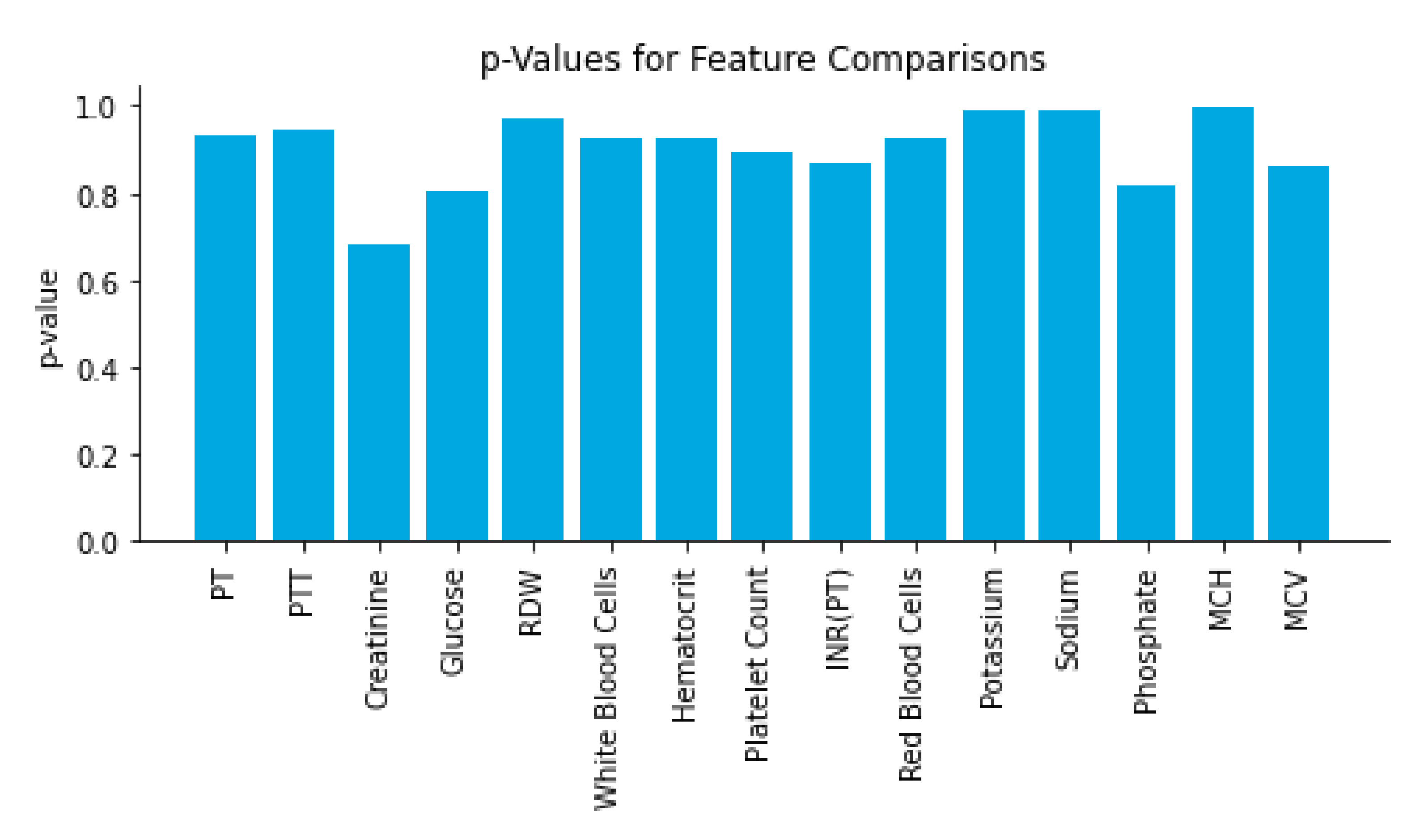
Several results support that the real and simulated data were essentially indistinguishable from each other. T-tests comparing a number of covariate distributions between the real and simulated data found highly insignificant
p-values (
p > 0.5 for all), indicating that the simulated and real data had indistinguishable covariate distributions (
Figure 2). Further, when trained to distinguish between the simulated and real patient data, the logistic regression-based adversary model displayed near-random performance for discrimination of real patient data. Across the five folds of data, the model demonstrated an average AUC
adversary of 0.50 ± 0.01 (
Supplementary Figure S1).
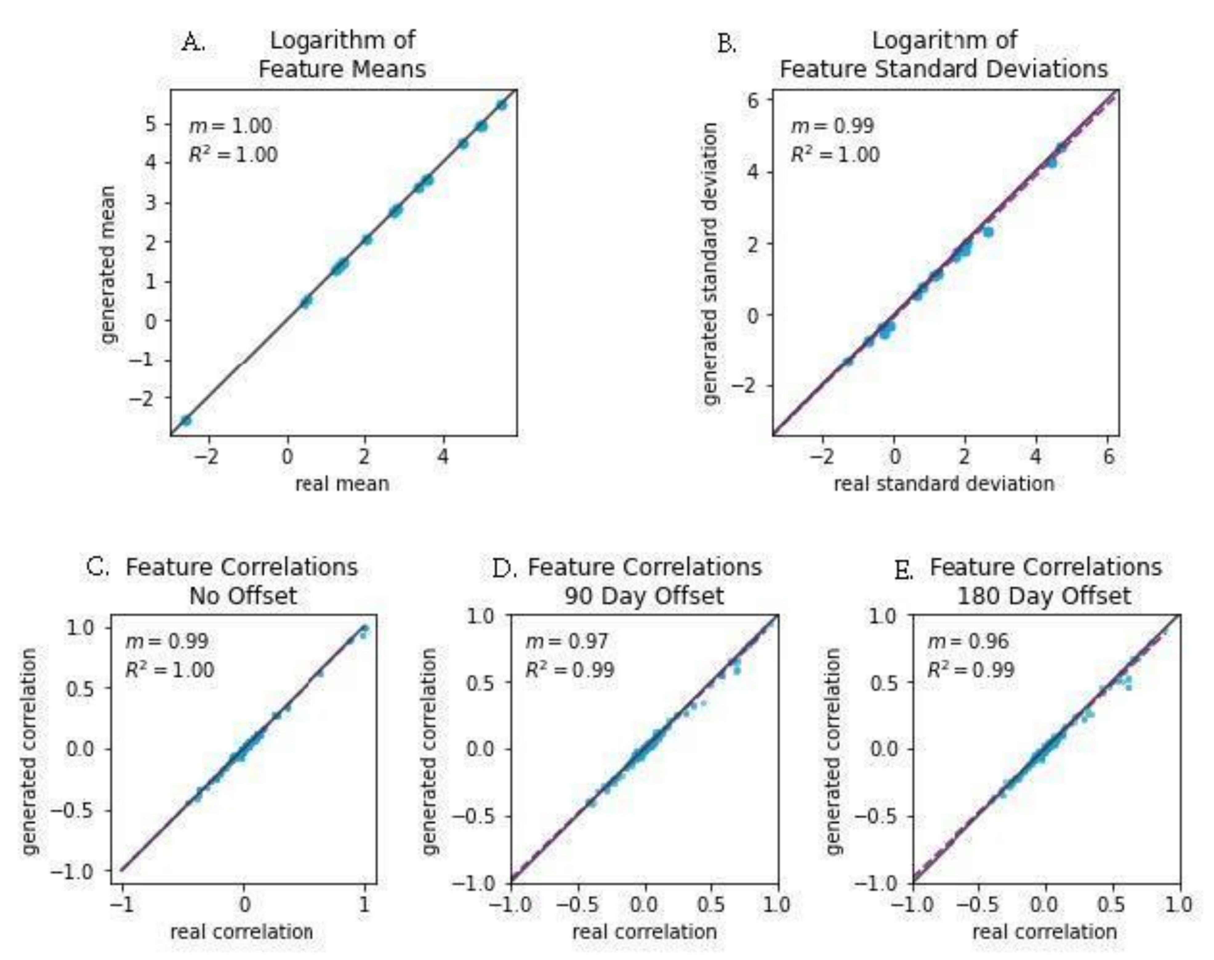
We also examined several correlations between aspects of the real and simulated data to further assess how well the simulated data mimicked the genuine patient data (
Figure 3). When the log-transformed means of each feature were compared between the real and simulated data, we observed a slope of 1.0 and a Pearson’s correlation coefficient of 1.0. Log-transformed feature standard deviations were slightly less strongly correlated, with a slope of 0.96 and a correlation coefficient of 0.99. When examining the correlations of feature correlations across several lag times, we also found evidence of strong correlations between the real and simulated data. At lags of 0, 90, and 180 days, we observed slopes of 0.99 (R
2 = 1.00), 0.97 (R
2 = 0.99), and 0.96 (R
2 = 0.99), respectively. In addition to strong correlations, the slope of near 1.0 for all pairs of measures indicated that the magnitude of values in the real and simulated data were nearly identical.
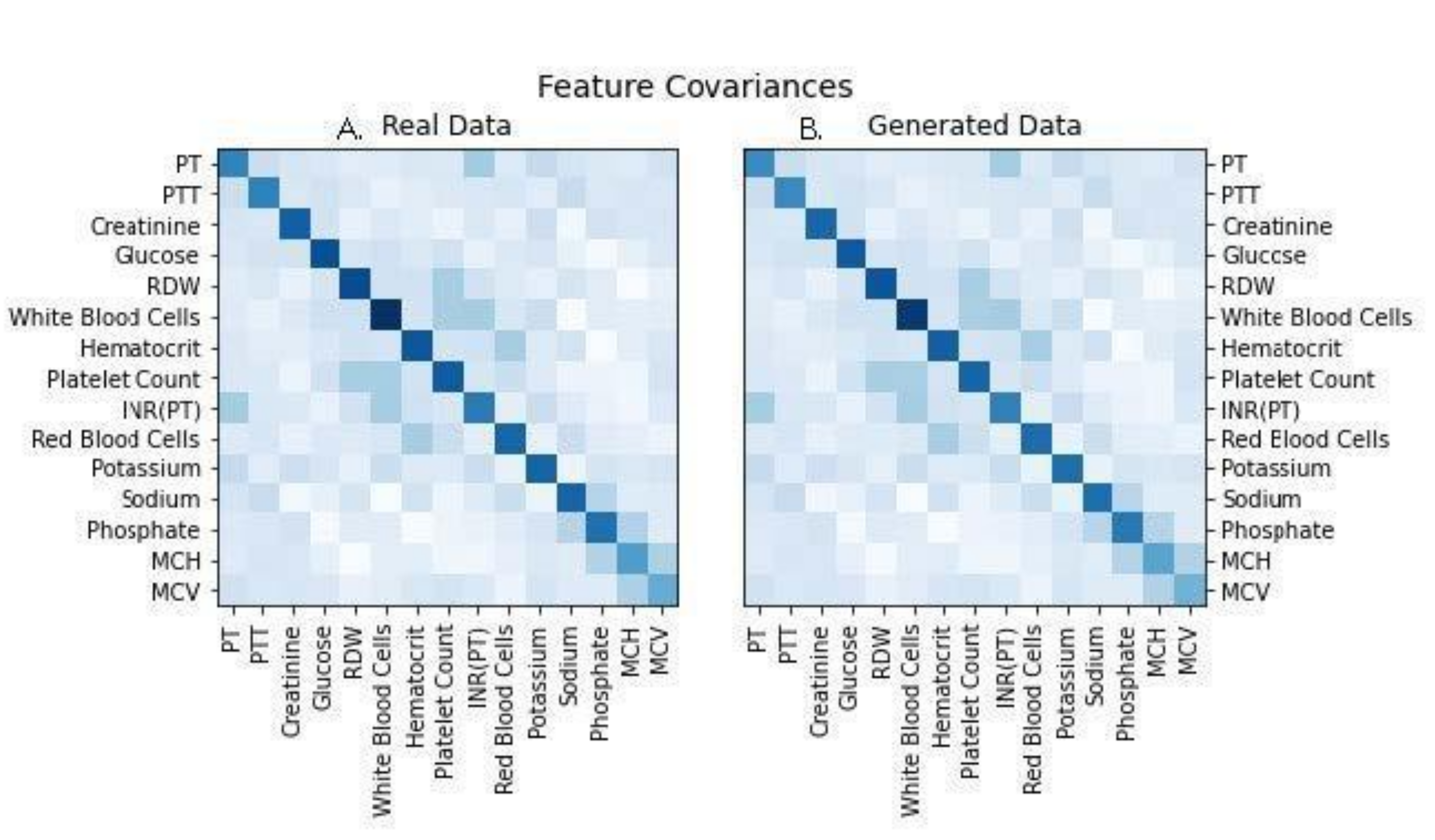
The real and simulated data also displayed nearly identical covariance structures, as shown in
Figure 4. Covariance structure similarity is important for ensuring that trends of disease progression found in models generated with real data will result in the same trends of disease progression as those found in models generated with simulated data. To more directly assess the accuracy of modeling with the simulated data we examined forecasted next measurements, where the last measure in a stream of real patient data was erased and projected through data simulation (
Figure 5). The simulated values fell within the range of observed patient measurements at later timesteps, indicating that projected values maintained many of the properties expected from longitudinal real-world data.
6. Discussion
In this paper, we present a variational autoencoder model to create a “digital twin” of data for patients who experienced an ischemic stroke. This method is capable of accurately capturing the cross-sectional and longitudinal properties of real patient data such that the stream of simulated data is statistically indistinguishable from real patient data, as shown by the results of the time-lagged correlation and projected next measure experiments. This work builds upon past developing digital twin models for forecasting of Alzheimer’s disease and multiple sclerosis progression [
3,
6].
In particular, our current work demonstrates that a digital twin model for forecasting the progression of relevant clinical measurements in patients at risk of ischemic stroke was virtually indistinguishable from real patient data under an adversarial ML discriminator. To ensure that the model was accurately learning the unimodal properties of the clinical features,
t-tests comparing real vs. synthetic features were run (
Figure 2). The resulting
p-values were larger than 0.6 for each feature, suggesting replication of these distributions. Linear regression to the means and standard deviations of real vs. synthetic data yielded strong fitting (
Figure 3A,B), with slope nearly 1.0 (R
2 ≥ 0.99); a model that perfectly replicates the real data would have a slope of exactly 1. In addition, statistical dependence between features in the generated data was measured using correlation between pairs of features in the generated and real trajectories. Linear regression to the paired data demonstrated strong fitting with a slope of 0.99 (R
2 ≥ 0.99). (
Figure 3C), indicating fidelity between synthetic data and actual data. Plots of the covariance structures of the feature values between real and synthetic data were virtually indistinguishable (
Figure 4), which also indicates accuracy in the trajectory of simulated data when compared against real patient data. Regression to real vs. synthetic time-lagged correlation values of feature pairs (
Figure 3D,E) indicates that the model replicates the statistical dependencies in the patients’ generated timelines as time progresses. To visualize the model’s effectiveness when generating long-term forecasts, clinical feature projections over 10 years into the future (using only the first 270 days of measurements) were plotted to further substantiate this finding (
Figure 5). This research fills a gap in knowledge regarding a tool that has the potential to be transformative for personalized medicine and patient care in that is presents a scalable solution that is operationally nimble and relies only upon readily available EHR data to overcome constraints that other digital twins models have reported due to data availability and practical operating requirements [
20,
21].
Digital twin models have marked value in the study of progressive neurological conditions like Alzheimer’s disease and multiple sclerosis. Neurological disorders are notoriously difficult to study due to the difficulty in determining onset time [
22], slow and unpredictable disease progression [
23], and the long follow-up times necessary to ascertain patient outcomes [
24]. These factors necessitate large and expensive trials [
24,
25,
26] and clearly illuminate the value of digital twin models for facilitating more efficient study of these diseases. Digital twin models also have applications for disease study beyond the setting of rare and slowly progressive conditions. Such models can be used to eliminate the need for control arms in clinical trials, allowing a digital twin of each patient to serve as their own control, thereby allowing a greater number of patients to benefit from treatment and increasing study power. In the case of ischemic stroke, in particular, a digital twin model could be used to assess a patient’s risk of incident or recurrent ischemic stroke with and without the use of prophylactic anticoagulant therapy [
27,
28].
The present work demonstrates proof of concept that digital twin models may be useful for forecasting relevant clinical trajectories for acute-onset conditions [
29,
30] and simulating disease progression. Estimation of disease progression using ML to simulate data has been examined in several research studies. Fisher et al. used an unsupervised ML model to create data simulating the trajectory of Alzheimer’s disease in individual patients [
3]. This study compared real and generated patient data, including the ADAS-Cog scale [
31] and Mini Mental State Exam (MMSE) [
32] scores. The authors found that generated patient data was virtually indistinguishable from real patient data both for composite disease severity scores and individual score components, thereby simulating entire disease trajectories [
3]. Another recent study by Walsh et al. examined the ability of simulated patient data (i.e., the “digital subject”) to forecast the trajectory of Multiple Sclerosis (MS), a disease similar to Alzheimer’s if only in its heterogenous and often complicated nature [
1]. Using clinical trial data from control subjects that are made available by the Multiple Sclerosis Outcome Assessments Consortium, the researchers created 1000 digital subjects for each patient dataset included in the study. The results of the study indicated that the actual patient data and simulated data could not be differentiated from one another by a ML model. Importantly, digital twin type simulations have also been used to simulate the immunogenic landscape of SARS-CoV-2 [
33], which may encourage the development of universal blueprints for COVID-19 vaccine designs.
Personalized medicine presents itself as a profound advancement of medical technology and clinical decision support tools. Potential risks related to the use of digital twins include those related to accuracy, data quality and usefulness [
2,
34,
35,
36], health equity [
35], the ability to incorporate these high-tech tools into existing infrastructure [
34,
36], and privacy [
2,
35,
36]. However, the potential value of this tool indicates a need for further exploration to uncover ways to minimize these pitfalls. Using a generative adversarial networks (GAN) model, Choi et al. has offered one potential solution to this issue of privacy by successfully using ML to develop synthetic patient data that mirrored the accuracy of predictive models that used real patient data [
37]. One concern may be that the training data can be replicated using the trained model, allowing leakage of patient information. VAEs sample from a distribution for each generated time example, and so have some but no direct coupling between training examples and generated examples. Using a GAN, as suggested in Choi et al., could further decouple the real patient information from the end model due to the different sampling and training mechanisms, potentially leading to greater privacy [
37].
There are several limitations of this work. First, the model was trained and tested on a small patient population. Only 244 unique patient encounters were used by the model after data processing and filtering, which may have impacted model performance. In future work it would be beneficial to validate model performance on larger data sets. It is also possible that log-transforming the lab features, while an attempt to bring the feature distributions closer to a normal distribution, may have inadvertently introduced skewness to the data. Another drawback is inherent to the binning process: it may be desirable that measurements occurring close to the boundaries of bins be accounted for by both in some way, with a smoother boundary than the one presented in this work. Additionally, the adversary model trained to distinguish between real and simulated data was developed using logistic regression. While these results suggested that real and simulated data were virtually indistinguishable, it is possible that an adversary model trained using more sophisticated ML methods would be able to better discriminate between the two data types. In addition, constraints of availability of relevant data limited our ability to choose model input features (e.g., no assessments of cognitive state were available in the data set, which if available could have been used by the model to inform patient trajectory forecasting.) Because this is a retrospective study, we also cannot determine the impact this model may have on patient care and management in live settings.
7. Conclusions
Despite its limitations, the machine learning model developed in this study shows promise as a necessary precision medicine approach to individualized forecasting of disease progression. However, as this type of modeling is still early in development in terms of its application in healthcare, it would benefit to validate its use in multiple settings with varying data types to determine its accuracy and effectiveness as a clinical decision support tool.
Generally, our work fills a knowledge gap in the area of digital twins, presenting exploratory research that lays the foundation for future research. Specifically, we have demonstrated that this software can be implemented with few infrastructure changes into existing EHR databases and use only EHR data to generate patient trajectory simulations with high accuracy. Our current work demonstrates that a digital twins model is able to accurately forecast clinical measurement trajectory in patients who went on to experience an ischemic stroke. Use of such a tool in live clinical settings may allow for tailored treatment to improve patient outcomes, and provide a low-cost, efficient method of conducting clinical trials.
Supplementary Materials
The following supplementary materials are available online at
https://www.mdpi.com/article/10.3390/app11125576/s1: Figure S1. A logistic regression adversary was trained on the test set to distinguish between real and simulated time window vectors. To do this, the test set was split with five-fold cross-validation. The adversary was trained on four of the chunks and tested on the last, and the ROC curve and AUROC score were recorded. The process was repeated 100 times for each of the five chunks used for testing.
Table S1. International Classification of Diseases (ICD) Ninth and Tenth Revision codes used to identify an ischemic stroke population.
Author Contributions
A.A. performed the data analysis for this work; A.A., G.B., E.P., A.S. and J.C. contributed to the drafting of this work; all authors contributed to the revision of this work; and A.A., R.D., J.C., Q.M. and H.B. contributed to the conception of this work. All authors have read and agreed to the published version of the manuscript.
Funding
There is no funding to report for this work.
Institutional Review Board Statement
Data were collected passively and de-identified in compliance with the Health Insurance Portability and Accountability 438 Act (HIPAA). Because data were de-identified and collected retrospectively, this study was considered non-human subjects research and did not require Institutional Review Board approval.
Informed Consent Statement
Not applicable.
Data Availability Statement
Restrictions apply to the availability of the patient data which were used under license for the current study, and so are not publicly available. The MLA code developed in this study is proprietary and not publicly available.
Conflicts of Interest
All authors who have affiliations listed with Dascena (Houston, TX, USA) are employees or contractors of Dascena.
Financial Disclosures
R.D., J.C., Q.M. own stock in Dascena. All other authors have no financial disclosures to report.
References
- Walsh, J.R.; Smith, A.M.; Pouliot, Y.; Li-Bland, D.; Loukianov, A.; Fisher, C.K. Consortium, for the M.S.O.A. Generating Digital Twins with Multiple Sclerosis Using Probabilistic Neural Networks. bioRxiv 2020. [Google Scholar] [CrossRef]
- Bruynseels, K.; De Sio, F.S.; Hoven, J.V.D. Digital Twins in Health Care: Ethical Implications of an Emerging Engineering Paradigm. Front. Genet. 2018, 9, 31. [Google Scholar] [CrossRef] [PubMed]
- Fisher, C.K.; Smith, A.M.; Walsh, J.R. Machine Learning for Comprehensive Forecasting of Alzheimer’s Disease Progression. Sci. Rep. 2019, 9, 13622. [Google Scholar] [CrossRef] [PubMed]
- Moser, A.; Appl, C.; Brüning, S.; Hass, V.C. Mechanistic Mathematical Models as a Basis for Digital Twins. Adv. Biochem. Eng. Biotechnol. 2020, 176, 133–180. [Google Scholar] [CrossRef]
- Gargalo, C.L.; Heras, S.C.D.L.; Jones, M.N.; Udugama, I.; Mansouri, S.S.; Krühne, U.; Gernaey, K.V. Towards the Development of Digital Twins for the Bio-manufacturing Industry. Blue Biotechnol. 2020, 1–34. [Google Scholar] [CrossRef]
- Croatti, A.; Gabellini, M.; Montagna, S.; Ricci, A. On the Integration of Agents and Digital Twins in Healthcare. J. Med. Syst. 2020, 44, 161. [Google Scholar] [CrossRef]
- Liu, Z.; Shi, G.; Zhang, A.; Huang, C. Intelligent Tensioning Method for Prestressed Cables Based on Digital Twins and Artificial Intelligence. Sensors 2020, 20, 7006. [Google Scholar] [CrossRef]
- JAMA Study First to Estimate Key Clinical Trial Costs. Available online: https://www.ismp.org/news/jama-study-first-estimate-key-clinical-trial-costs (accessed on 6 January 2021).
- Björnsson, B.; Borrebaeck, C.; Elander, N.; Gasslander, T.; Gawel, D.R.; Gustafsson, M.; Jörnsten, R.; Lee, E.J.; Li, X.; Lilja, S.; et al. Digital twins to personalize medicine. Genome Med. 2020, 12, 4. [Google Scholar] [CrossRef]
- Digital Twin ConsortiumTM. Available online: https://themeforest.net/user/dan_fisher and https://www.digitaltwinconsortium.org (accessed on 18 May 2021).
- Rao, D.J.; Mane, S. Digital Twin Approach to Clinical DSS with Explainable AI. arXiv 2019, arXiv:1910.13520. [Google Scholar]
- Laubenbacher, R.; Sluka, J.P.; Glazier, J.A. Using digital twins in viral infection. Science 2021, 371, 1105–1106. [Google Scholar] [CrossRef]
- Donkor, E.S. Stroke in the 21st Century: A Snapshot of the Burden, Epidemiology, and Quality of Life. Stroke Res. Treat. 2018, 2018, 3238165. [Google Scholar] [CrossRef]
- Zhang, Y.; Zhou, Y.; Zhang, D.; Song, W. A Stroke Risk Detection: Improving Hybrid Feature Selection Method. J. Med. Internet Res. 2019, 21, e12437. [Google Scholar] [CrossRef] [PubMed]
- Higgins, I.; Matthey, L.; Pal, A.; Burgess, C.; Glorot, X.; Botvinick, M.; Mohamed, S.; Lerchner, A. Beta-VAE: Learning Basic Visual Concepts with a Constrained Variational Framework. In Proceedings of the ICLR 2017, Toulon, France, 24–26 April 2017. [Google Scholar]
- Kingma, D.P.; Welling, M. Auto-Encoding Variational Bayes. arXiv. 2014. Available online: http://arxiv.org/abs/1312.6114 (accessed on 8 June 2021).
- Johnson, A.; Bulgarelli, L.; Pollard, T.; Horng, S.; Celi, L.A.; Mark, R. MIMIC-IV. PhysioNet 2020. [Google Scholar] [CrossRef]
- Hall, R.; Mondor, L.; Porter, J.; Fang, J.; Kapral, M.K. Accuracy of Administrative Data for the Coding of Acute Stroke and TIAs. Can. J. Neurol. Sci. J. Can. Sci. Neurol. 2016, 43, 765–773. [Google Scholar] [CrossRef]
- Federal Policy for the Protection of Human Subjects (Common Rule). Available online: https://www.hhs.gov/ohrp/regulations-and-policy/regulations/common-rule/index.html (accessed on 18 May 2021).
- Khan, S.; Yairi, T. A review on the application of deep learning in system health management. Mech. Syst. Signal Process. 2018, 107, 241–265. [Google Scholar] [CrossRef]
- Booyse, W.; Wilke, D.N.; Heyns, S. Deep digital twins for detection, diagnostics and prognostics. Mech. Syst. Signal Process. 2020, 140, 106612. [Google Scholar] [CrossRef]
- Dubois, B.; Hampel, H.; Feldman, H.H.; Scheltens, P.; Aisen, P.; Andrieu, S.; Bakardjian, H.; Benali, H.; Bertram, L.; Blennow, K.; et al. Preclinical Alzheimer’s disease: Definition, natural history, and diagnostic criteria. Alzheimer’s Dement. J. Alzheimer’s Assoc. 2016, 12, 292–323. [Google Scholar] [CrossRef]
- Reich, D.S.; Lucchinetti, C.F.; Calabresi, P.A. Multiple Sclerosis. N. Engl. J. Med. 2018, 378, 169–180. Available online: https://www.nejm.org/doi/full/10.1056/NEJMra1401483 (accessed on 8 June 2021). [CrossRef] [PubMed]
- Hyland, M.A.; Rudick, R. Challenges to clinical trials in multiple sclerosis: Outcome measures in the era of disease-modifying drugs. Curr. Opin. Neurol. 2011, 24, 255–261. [Google Scholar] [CrossRef] [PubMed]
- NIA-Funded Active Alzheimer’s and Related Dementias Clinical Trials and Studies. Available online: http://www.nia.nih.gov/research/ongoing-AD-trials (accessed on 16 December 2020).
- Connick, P.; De Angelis, F.A.; Parker, R.; Plantone, D.; Doshi, A.; John, N.; Stutters, J.; MacManus, D.; Carrasco, F.P.; Barkhof, F.; et al. Multiple Sclerosis-Secondary Progressive Multi-Arm Randomisation Trial (MS-SMART): A multiarm phase IIb randomised, double-blind, placebo-controlled clinical trial comparing the efficacy of three neuroprotective drugs in secondary progressive multiple sclerosis. BMJ Open 2018, 8, e021944. [Google Scholar] [CrossRef]
- Amin, A. Oral anticoagulation to reduce risk of stroke in patients with atrial fibrillation: Current and future therapies. Clin. Interv. Aging 2013, 8, 75–84. [Google Scholar] [CrossRef][Green Version]
- Abbas, M.; Malicke, D.T.; Schramski, J.T. Stroke Anticoagulation; StatPearls Publishing: Treasure Island, FL, USA, 2020. [Google Scholar]
- Martinez-Velazquez, R.; Gamez, R.; El Saddik, A. Cardio Twin: A Digital Twin of the human heart running on the edge. In Proceedings of the 2019 IEEE International Symposium on Medical Measurements and Applications, Istanbul, Turkey, 26–28 June 2019; pp. 1–6. [Google Scholar] [CrossRef]
- Lal, A.; Li, G.; Cubro, E.; Chalmers, S.; Li, H.; Herasevich, V.; Dong, Y.; Pickering, B.W.; Kilickaya, O.; Gajic, O. Development and Verification of a Digital Twin Patient Model to Predict Specific Treatment Response During the First 24 Hours of Sepsis. Crit. Care Explor. 2020, 2, e0249. [Google Scholar] [CrossRef] [PubMed]
- Rosen, W.G.; Mohs, R.C.; Davis, K.L. A new rating scale for Alzheimer’s disease. Am. J. Psychiatry 1984, 141, 1356–1364. [Google Scholar] [CrossRef]
- Folstein, M.F.; Folstein, S.E.; McHugh, P.R. “Mini-mental state”. A practical method for grading the cognitive state of patients for the clinician. J. Psychiatr. Res. 1975, 12, 189–198. [Google Scholar] [CrossRef]
- Malone, B.; Simovski, B.; Moliné, C.; Cheng, J.; Gheorghe, M.; Fontenelle, H.; Vardaxis, I.; Tennøe, S.; Malmberg, J.-A.; Stratford, R.; et al. Artificial intelligence predicts the immunogenic landscape of SARS-CoV-2 leading to universal blueprints for vaccine designs. Sci. Rep. 2020, 10, 22375. [Google Scholar] [CrossRef] [PubMed]
- Fuller, A.; Fan, Z.; Day, C.; Barlow, C. Digital Twin: Enabling Technologies, Challenges and Open Research. IEEE Access 2020, 8, 108952–108971. [Google Scholar] [CrossRef]
- Digital Twins for Personalized Medicine—A Critical Assessment. Available online: https://diginomica.com/digital-twins-personalized-medicine-critical-assessment (accessed on 6 January 2021).
- Corral-Acero, J.; Margara, F.; Marciniak, M.; Rodero, C.; Loncaric, F.; Feng, Y.; Gilbert, A.; Fernandes, J.F.A.; Bukhari, H.; Wajdan, A.; et al. The ‘Digital Twin’ to enable the vision of precision cardiology. Eur. Hear. J. 2020, 41, 4556–4564. [Google Scholar] [CrossRef]
- Choi, E.; Biswal, S.; Malin, B.; Duke, J.; Stewart, W.F.; Sun, J. Generating Multi-Label Discrete Patient Records Using Generative Adversarial Networks. arXiv 2018, arXiv:170306490. [Google Scholar]
| Publisher’s Note: MDPI stays neutral with regard to jurisdictional claims in published maps and institutional affiliations. |
© 2021 by the authors. Licensee MDPI, Basel, Switzerland. This article is an open access article distributed under the terms and conditions of the Creative Commons Attribution (CC BY) license (https://creativecommons.org/licenses/by/4.0/).


 ,
, 


