A Multiple and Multi-Level Substructure Method for the Dynamics of Complex Structures

Abstract

Based on the fixed interface component mode synthesis, a multiple and multi-level substructure method for the modeling of complex structures is proposed in this paper. Firstly, the residual structure is selected according to the structural characteristics of the assembled complex structure. Secondly, according to the assembly relationship, the parts assembled with the residual structure are divided into a group of substructures, which are named the first-level substructure, the parts assembled with the first-level substructure are divided into a second-level substructure, and consequently the multi-level substructure model is established. Next, the substructures are dynamically condensed and assembled on the boundary of the residual structure. Finally, the substructure system matrix, which is replicated from the matrix of repeated physical geometry, is obtained by preserving the main modes and the constrained modes and the system matrix of the last level of the substructure is assembled to the upper level of the substructure, one level up, until it is assembled in the residual structure. In this paper, an assembly structure with three panels and a gear box is adopted to verify the method by simulation and a rotor is used to experimentally verify the method. The results show that the proposed multiple and multi-level substructure modeling method is not unique to the selection of residual structures, and different classification methods do not affect the calculation accuracy. The selection of 50% external nodes can further improve the analysis efficiency while ensuring the calculation accuracy.

1. Introduction

The modeling of a complex structure and the conduction of accurate dynamics analysis is always time-consuming. The established model based on a traditional finite element method is not efficient in calculations, especially for large and complex structures, such as spacecraft and aircraft structures. In addition, various uncertain factors in the modeling process leads to errors in the computational results. Therefore, it is necessary to propose methods to improve modeling efficiency while considering modeling accuracy. For complex and huge-degrees-of-freedom systems, a substructure method is a good choice [1,2].

The substructure is obtained by projecting the dynamics of a linear finite element model to a low-dimensional subspace spanned by so-called component modes. The component mode can be a collection of various modes, such as a rigid body mode, a normal mode, and a constrained mode [3,4]. In recent years, the introduction and application of substructure methods in the static and dynamic analysis of different structural systems have been developed [5,6]. Bai et al. [7,8,9] used the improved substructure component mode synthesis based on the extremum response surface method to improve the computational efficiency and reliability of atomized turbine blade disc vibration characteristics. With the help of substructure technology, Gu [10]used the wave packet method to effectively evaluate the heat conduction of each phonon mode in the large-period harmonic lattice. Duan et al. [11] developed a model simplification technique which can efficiently calculate and accurately analyze the forced response displacement and stress amplitude levels of a blade disc that vibrates in the high frequency range. Jung et al. [12] used a hybrid-interface method based on component mode synthesis to develop a reduced-order model (ROM) for tuning systems with splines. Using these valid ROMs in forced response analysis, it was found that the new modeling method could save computational costs, while ensuring good accuracy compared to full-order finite element analysis. Zhu et al. [13] proposed an improved substructure-based response sensitivity method to accelerate the convergence rate of model updating. The accuracy and efficiency of the proposed method was tested by two numerical simulations and an experimental case. Tian et al. [14,15,16] used a new iterative reduced-order substructure method to calculate the eigen-solutions and eigen-sensitivities of the global structure. By using this method, the eigen-solutions and eigen-sensitivities of the whole structure can be accurately calculated with only a few substructural eigenmodes and several iterations. Weng et al. [17,18] proposed a substructure-based finite element model updating technique. This method was applied to frame structures and actual Bridges, and the computation of traditional model updating methods performed on global structures was reduced. Shamloofard et al. [19] proposed a new shell super-element for studying linear/nonlinear static and free vibration analysis of spherical structures with partial or complete spherical geometry. The results showed that the supercell can achieve high precision with low computational costs. Fatan et al. [20] used a new cylindrical super-element for the design and vibration analysis of FGM rings to obtain the natural frequencies and modal shapes, and compared the results with simple cases obtained from analytical solutions and conventional elements. Considering a few newly designed super-elements, comparable results for simple cases in the reported literature can be achieved. Plaza et al. [21] proposed several models to analyze the load distribution and the deformation of slewing support components in wind turbine generators. This work presented a super-element-based FE model that can significantly reduce computational costs with a negligible loss of precision. Tuysuz et al. [22,23] proposed a new substructure order reduction method with high computational efficiency. The order of the initial structure was reduced by deleting the order of the substructure and the model. In the second year, the initial structure and the residual structure of the dynamic order reduction workpiece were obtained by using the model order reduction technique. Cao et al. [24,25,26] proposed a model modification method based on the residual flexible mixed boundary substructure method. The interface elastic parameters of the bolted joints were identified by using the experimental data. The results showed that this method has good performance of finite element model correction. Geradin et al. [27] came up with a "node-less" super-element formulation based on a two-component mode synthesis, which provides a high computational efficiency for applications in structural dynamics and flexible multi-body dynamics. Voormeeren et al. [28] combined super-element modeling with the concept of modal truncation augmentation to extend the reduction basis by adding residual vectors. The proposed enhanced super-element approach allows for the creation of compact and accurate models of complex support structures for efficient integrated simulation of offshore wind turbines. It is found that the most obvious advantage of the substructure is that it can improve the computational efficiency while ensuring the accuracy. Therefore, for complex structures, the method of the substructure can greatly reduce the computation time. For the concrete use of the substructure, part of the research content can be implemented.

Among substructure methods, component mode synthesis is the most widely used. Based on the component mode synthesis of a fixed interface [29,30], the theoretical formula for the multi-level substructure method is derived in this paper. Taking the assembly structure with three panels, the gear box of a helicopter and the combustion rotor of a aeroengine as the research objects, the dynamic models were established and the dynamic characteristics were analyzed based on the multi-level substructures. At the same time, the influences of different classification methods, the selection of residual structures, and the selection of external nodes on the calculation accuracy were explored.

2. Component Mode Synthesis of Fixed Interface

For undamped systems, the dynamic system equation can be written as follows:

$$\mathbf{M}\ddot{\mathbf{u}}+\mathbf{K}\mathbf{u}=\mathbf{F}$$

(1)

In the formula, M is the mass matrix, K is the stiffness matrix, u is the displacement vector, F is the external force vector, and $\ddot{\mathbf{u}}$ represents the second derivative of displacement.

All the degrees of freedom of the system are divided into two parts:

• The part that is not connected with other substructures (internal degrees of freedom), denoted as {u_o}.
• The part connected with other substructures (external degree of freedom or boundary degree of freedom) is denoted as {u_a}.

According to the partition of external and internal degrees of freedom, Equation (1) can be written as follows:

$$\left[\begin{array}{cc}{\mathbf{M}}_{\mathrm{oo}}& {\mathbf{M}}_{\mathrm{oa}}\\ {\mathbf{M}}_{\mathrm{ao}}& {\mathbf{M}}_{\mathrm{aa}}\end{array}\right]\left[\begin{array}{c}{\ddot{\mathbf{u}}}_{\mathrm{o}}\\ {\ddot{\mathbf{u}}}_{\mathrm{a}}\end{array}\right]+\left[\begin{array}{cc}{\mathbf{K}}_{\mathrm{oo}}& {\mathbf{K}}_{\mathrm{oa}}\\ {\mathbf{K}}_{\mathrm{ao}}& {\mathbf{K}}_{\mathrm{aa}}\end{array}\right]\left[\begin{array}{c}{\mathbf{u}}_{\mathrm{o}}\\ {\mathbf{u}}_{\mathrm{a}}\end{array}\right]=\left[\begin{array}{c}{\mathbf{F}}_{\mathrm{o}}\\ {\mathbf{F}}_{\mathrm{a}}\end{array}\right]$$

(2)

In the problem of solving the eigenvalues of the system, F_O = 0, F_a = F_0ae^iωt, u = Ue^iωt. F₀ represents the amplitude of the external force vector, U is the amplitude of the displacement response. In this regard, Equation (2) can be written as follows:

$$\left(\left[\begin{array}{cc}{K}_{\mathrm{oo}}& K_{\mathrm{oa}}\\ K_{\mathrm{ao}}& K_{\mathrm{aa}}\end{array}\right]-{\omega }^2\left[\begin{array}{cc}{\mathbf{M}}_{oo}& {\mathbf{M}}_{\mathrm{oa}}\\ {\mathbf{M}}_{\mathrm{ao}}& {\mathbf{M}}_{\mathrm{aa}}\end{array}\right]\right)\left[\begin{array}{c}{U}_{\mathrm{o}}\\ U_{\mathrm{a}}\end{array}\right]=\left[\begin{array}{c}\mathbf{0}\\ F_{0\mathrm{a}}\end{array}\right]$$

(3)

In the formula, ω represents the circular frequency (in rad/s) of the structure.

When the interface surface is constrained, U_a = 0 is substituted into the first equation of Equation (3) to obtain the following eigenvalue equation of the interface:

$$\left(K_{\mathrm{oo}}-{\omega }^2{\mathbf{M}}_{\mathrm{oo}}\right)U_{\mathrm{o}}=\mathbf{0}$$

(4)

Therefore, the eigenvalue equation of the interface corresponding to Equation (4) is ${\overline{\mathsf{\phi }}}_{\mathrm{bL}}$, and the eigenvalue matrix is A_bL, then the main mode ${\mathsf{\phi }}_{\mathrm{bL}}$ is as follows

$${\mathsf{\phi }}_{\mathrm{bL}}=\left[\begin{array}{c}{\overline{\mathsf{\phi }}}_{\mathrm{bL}}\\ \mathbf{0}\end{array}\right]$$

(5)

Assuming that ${\overline{\mathbf{N}}}_0$ is made up of ${\mathsf{\phi }}_{\mathrm{bL}}$ and Φ_c0, then ${\overline{\mathbf{N}}}_0$ can be written as follows

$${\overline{\mathbf{N}}}_0=\left[\begin{array}{cc}{\Phi }_{\mathrm{c}0}& {\mathsf{\phi }}_{\mathrm{bL}}\end{array}\right]$$

(6)

Among them, ${\overline{\mathbf{N}}}_0$ is the matrix of the first coordinate change of the substructure, ${\mathsf{\phi }}_{\mathrm{bL}}$ is the main mode reserved by the substructure constrained interface, and Φ_c0 is the constrained mode of all the interface degrees of freedom.

Ignoring the inertial force term in Formula (3), the static force equation is given as follows:

$$\left[\begin{array}{cc}{K}_{\mathrm{oo}}& K_{\mathrm{oa}}\\ K_{\mathrm{ao}}& K_{\mathrm{aa}}\end{array}\right]\left[\begin{array}{c}{\mathbf{U}}_{\mathrm{o}}\\ {\mathbf{U}}_{\mathrm{a}}\end{array}\right]=\left[\begin{array}{c}\mathbf{0}\\ {\mathbf{F}}_{0\mathrm{a}}\end{array}\right]$$

(7)

Solving the first equation of Equation (7), we get:

$${\mathbf{U}}_{\mathrm{o}}=-{\mathbf{K}}_{\mathrm{oo}}^{-1}{\mathbf{K}}_{\mathrm{oa}}{\mathbf{U}}_{\mathrm{a}}={\mathbf{t}}_{\mathrm{c}0}{\mathbf{U}}_{\mathrm{a}}$$

(8)

In the formula, t_c0 can be written as follows:

$${\mathbf{t}}_{\mathrm{c}0}=-{\mathbf{K}}_{\mathrm{oo}}^{-1}{\mathbf{K}}_{\mathrm{oa}}$$

(9)

Therefore, the static displacement U can be written as follows:

$$\mathbf{U}=\left[\begin{array}{c}{\mathbf{U}}_{\mathrm{o}}\\ {\mathbf{U}}_{\mathrm{a}}\end{array}\right]=\left[\begin{array}{c}{\mathbf{t}}_{\mathrm{c}0}\\ \mathbf{I}\end{array}\right]{\mathbf{U}}_{\mathrm{a}}={\mathbf{\Phi }}_{\mathrm{c}0}{\mathbf{U}}_{\mathrm{a}}$$

(10)

$${\Phi }_{\mathrm{c}0}=\left[\begin{array}{c}{t}_{\mathrm{c}0}\\ I\end{array}\right]$$

(11)

Among them, Φ_c0 is the substructure interface constraint modal matrix, and I represents the identity matrix.

Therefore, the modal set ${\overline{\mathbf{N}}}_0$ can be written as follows

$${\overline{\mathbf{N}}}_0=\left[\begin{array}{cc}{\Phi }_{\mathrm{c}0}& {\mathsf{\phi }}_{\mathrm{bL}}\end{array}\right]=\left[\begin{array}{cc}{t}_{\mathrm{c}0}& {\overline{\mathsf{\phi }}}_{\mathrm{bL}}\\ I& 0\end{array}\right]$$

(12)

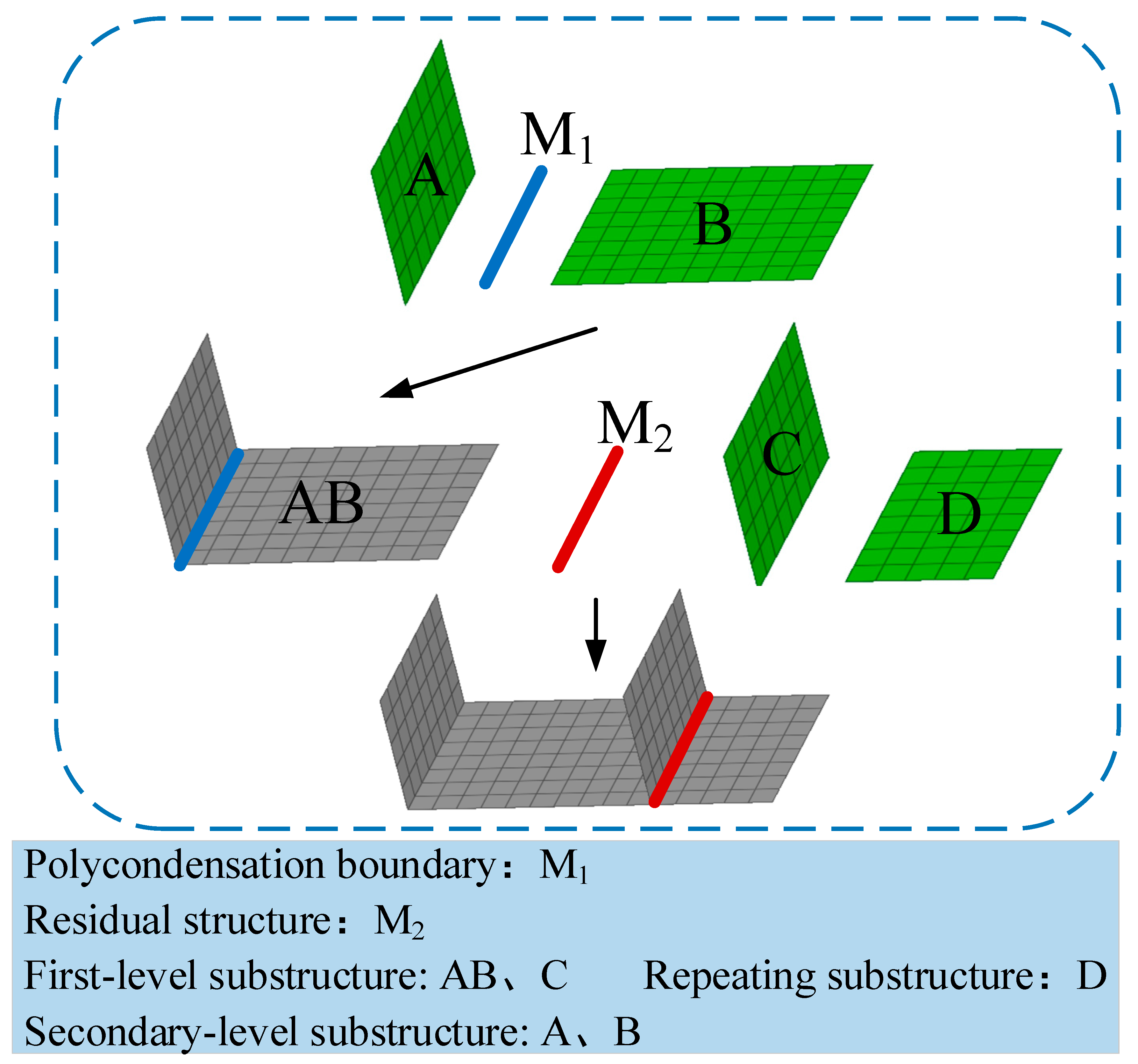
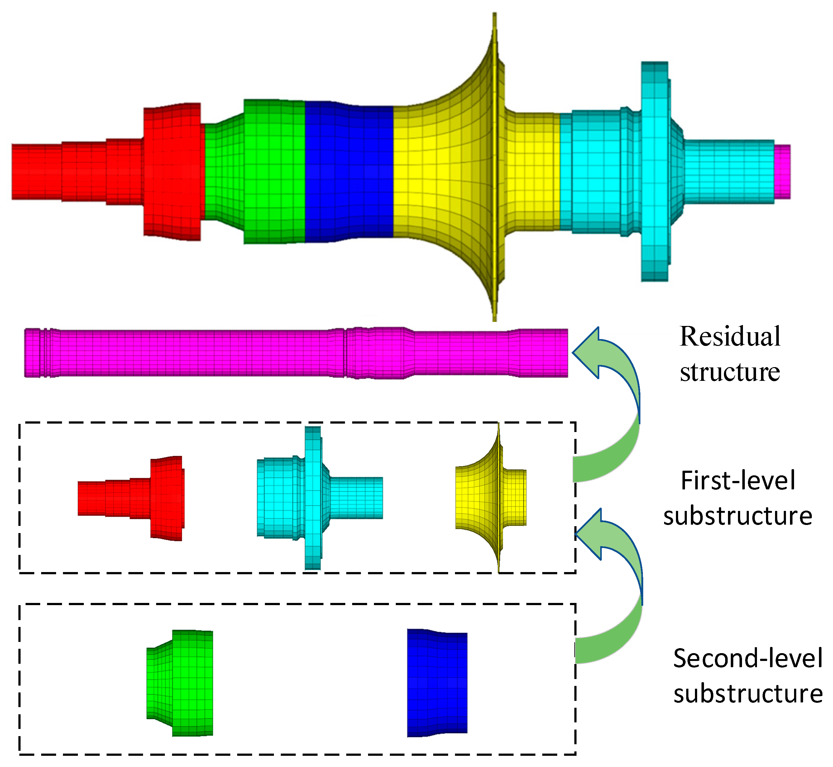
3. Multiple and Multi-Level Substructure Method

Figure 1 shows the schematic diagram of multiple and multi-level substructure. According to the interface displacement coordination equations $u_{\mathrm{a}}^{\mathrm{C}}=u_{\mathrm{a}}^{\mathrm{resC}}$, $u_{\mathrm{a}}^{\mathrm{D}}=u_{\mathrm{a}}^{\mathrm{resD}}$, $u_{\mathrm{a}}^{\mathrm{A}}=u_{\mathrm{a}}^{\mathrm{BA}}$ and $u_{\mathrm{a}}^{\mathrm{Bres}}=u_{\mathrm{a}}^{\mathrm{resB}}$(superscript resn represents the coupling form of residual structure and substructure n, n is the substructure code; the superscript BA indicates the coupling form of substructure B and substructure A), namely $p_{\mathrm{a}}^{\mathrm{C}}=p_{\mathrm{a}}^{\mathrm{resC}}$, $p_{\mathrm{a}}^{\mathrm{D}}=p_{\mathrm{a}}^{\mathrm{resD}}$, $p_{\mathrm{a}}^{\mathrm{A}}=p_{\mathrm{a}}^{\mathrm{BA}}$ and $p_{\mathrm{a}}^{\mathrm{Bres}}=p_{\mathrm{a}}^{\mathrm{resB}}$. Performing the second coordinate change we can get:

$$\left[\begin{array}{c}{p}_{\mathrm{o}}^{\mathrm{k}}\\ p_{\mathrm{a}}^{\mathrm{k}}\\ p_{\mathrm{o}}^{\mathrm{res}}\\ p_{\mathrm{a}}^{\mathrm{resk}}\end{array}\right]=\left[\begin{array}{ccc}I& 0& 0\\ 0& I& 0\\ 0& I& 0\\ 0& 0& I\end{array}\right]\left[\begin{array}{c}{q}_{\mathrm{o}}^{\mathrm{k}}\\ q_{\mathrm{a}}^{\mathrm{k}}\\ q_{\mathrm{o}}^{\mathrm{res}}\end{array}\right]$$

(13)

Among them, p represents modal coordinates, β represents the second coordinate transformation matrix, q represents generalized coordinates, superscript k (k = A, B, C, D) and res represent substructure k and the residual structure respectively, superscript resk represents the coupling form of residual structure and substructure k the subscripts o and a represent the form of internal degrees of freedom and the form of external degrees of freedom, respectively.

The dynamic polycondensation of substructure k is as follows

$${\overline{\mathbf{M}}}_{\mathrm{d}0}^{\mathrm{k}}={\left({\mathsf{\beta }}^{\mathrm{k}}\right)}^{\mathrm{T}}{\overline{\mathbf{N}}}_0^{\mathrm{T}}{\mathbf{M}}^{\mathrm{k}}{\overline{\mathbf{N}}}_0{\mathsf{\beta }}^{\mathrm{k}}$$

(14)

$${\overline{K}}_{\mathrm{d}0}^{\mathrm{k}}={\left({\mathsf{\beta }}^{\mathrm{k}}\right)}^{\mathrm{T}}{\overline{\mathbf{N}}}_0^{\mathrm{T}}{K}^{\mathrm{k}}{\overline{\mathbf{N}}}_0{\mathsf{\beta }}^{\mathrm{k}}$$

(15)

$${\mathbf{M}}^{\mathrm{k}}=\left[\begin{array}{cc}{\mathbf{M}}_{\mathrm{oo}}^{\mathrm{k}}& {\mathbf{M}}_{\mathrm{oa}}^{\mathrm{k}}\\ {\mathbf{M}}_{\mathrm{ao}}^{\mathrm{k}}& {\mathbf{M}}_{\mathrm{aa}}^{\mathrm{k}}\end{array}\right]$$

(16)

$$K^{\mathrm{k}}=\left[\begin{array}{cc}{K}_{\mathrm{oo}}^{\mathrm{k}}& K_{\mathrm{oa}}^{\mathrm{k}}\\ K_{\mathrm{ao}}^{\mathrm{k}}& K_{\mathrm{aa}}^{\mathrm{k}}\end{array}\right]$$

(17)

In the formula, ${\overline{\mathbf{M}}}_{\mathrm{d}0}^{\mathrm{k}}$ represents the mass matrix of the substructure k (k = A, B, C, D) after dynamic condensation, ${\overline{K}}_{\mathrm{d}0}^{\mathrm{k}}$ represents the stiffness matrix of the substructure k after dynamic condensation, M^k represents the mass matrix of the substructure k, and K^k represents the stiffness matrix of the substructure k.

Assembled, substructure AB, substructure C, and substructure D have the residual structure res. Therefore, the undamped free vibration equation of the system is as follows:

$${\overline{\mathbf{M}}}_{\mathrm{z}}\ddot{u}+{\overline{K}}_{\mathrm{z}}u=0$$

(18)

$${\overline{\mathbf{M}}}_{\mathrm{z}}={\mathbf{M}}^{\mathrm{res}}+{\overline{\mathbf{M}}}_{\mathrm{d}0}^{\mathrm{B}}+{\overline{\mathbf{M}}}_{\mathrm{d}0}^{\mathrm{C}}+{\overline{\mathbf{M}}}_{\mathrm{d}0}^{{\mathrm{D}}^{\prime }}$$

(19)

$${\overline{K}}_{\mathrm{z}}=K^{\mathrm{res}}+{\overline{K}}_{\mathrm{d}0}^{\mathrm{B}}+{\overline{K}}_{\mathrm{d}0}^{\mathrm{C}}+{\overline{K}}_{\mathrm{d}0}^{{\mathrm{D}}^{\prime }}$$

(20)

$${\mathbf{M}}^{\mathrm{B}}=\left[\begin{array}{ccc}{\mathbf{M}}_{\mathrm{oo}}^{\mathrm{A}}& {\mathbf{M}}_{\mathrm{oa}}^{\mathrm{A}}& 0\\ {\mathbf{M}}_{\mathrm{ao}}^{\mathrm{A}}& {\mathbf{M}}_{\mathrm{aa}}^{\mathrm{A}}+{\mathbf{M}}_{\mathrm{aa}}^{\mathrm{B}}& {\mathbf{M}}_{\mathrm{oa}}^{\mathrm{B}}\\ 0& {\mathbf{M}}_{\mathrm{ao}}^{\mathrm{B}}& {\mathbf{M}}_{\mathrm{oo}}^{\mathrm{B}}\end{array}\right]$$

(21)

$$K^{\mathrm{B}}=\left[\begin{array}{ccc}{K}_{\mathrm{oo}}^{\mathrm{A}}& K_{\mathrm{oa}}^{\mathrm{A}}& 0\\ K_{\mathrm{ao}}^{\mathrm{A}}& K_{\mathrm{aa}}^{\mathrm{A}}+K_{\mathrm{aa}}^{\mathrm{B}}& K_{\mathrm{oa}}^{\mathrm{B}}\\ 0& K_{\mathrm{ao}}^{\mathrm{B}}& K_{\mathrm{aa}}^{\mathrm{B}}\end{array}\right]$$

(22)

$${\mathbf{M}}^{\mathrm{res}}=\left[\begin{array}{cc}{\mathbf{M}}_{\mathrm{oo}}^{\mathrm{res}}& {\mathbf{M}}_{\mathrm{oa}}^{\mathrm{res}}\\ {\mathbf{M}}_{\mathrm{ao}}^{\mathrm{res}}& {\mathbf{M}}_{\mathrm{aa}}^{\mathrm{res}}\end{array}\right]$$

(23)

$$K^{\mathrm{res}}=\left[\begin{array}{cc}{K}_{\mathrm{oo}}^{\mathrm{res}}& K_{\mathrm{oa}}^{\mathrm{res}}\\ K_{\mathrm{ao}}^{\mathrm{res}}& K_{\mathrm{aa}}^{\mathrm{res}}\end{array}\right]$$

(24)

$${\overline{\mathbf{M}}}_{\mathrm{d}0}^{{\mathrm{D}}^{\prime }}=q^{\mathrm{T}}{\overline{\mathbf{N}}}_0^{\mathrm{T}}{\mathbf{M}}^{{\mathrm{D}}^{\prime }}{\overline{\mathbf{N}}}_{0}q$$

(25)

$${\overline{K}}_{\mathrm{d}0}^{{\mathrm{D}}^{\prime }}=q^{\mathrm{T}}{\overline{\mathbf{N}}}_0^{\mathrm{T}}{K}^{{\mathrm{D}}^{\prime }}{\overline{\mathbf{N}}}_{0}q$$

(26)

$${\mathbf{M}}^{{}_{{}^{{\mathrm{D}}^{\prime }}}}=\left[\begin{array}{cc}{\mathbf{M}}_{\mathrm{oo}}^{\mathrm{D}}& {\mathbf{M}}_{\mathrm{oa}}^{\mathrm{D}}\\ {\mathbf{M}}_{\mathrm{ao}}^{\mathrm{D}}& {\mathbf{M}}_{\mathrm{aa}}^{\mathrm{C}}\end{array}\right]$$

(27)

$$K^{{}^{{}_{{\mathrm{D}}^{\prime }}}}=\left[\begin{array}{cc}{K}_{\mathrm{oo}}^{\mathrm{D}}& K_{\mathrm{oa}}^{\mathrm{D}}\\ K_{\mathrm{ao}}^{\mathrm{D}}& K_{\mathrm{aa}}^{\mathrm{C}}\end{array}\right]$$

(28)

${\overline{\mathbf{M}}}_{\mathrm{z}}$ represents the mass matrix of the system, ${\overline{K}}_{\mathrm{z}}$ represents the stiffness matrix of the system, M^res represents the mass matrix of the residual structure res, K^res represents the stiffness matrix of the residual structure res, ${\overline{\mathbf{M}}}_{\mathrm{d}0}^{{\mathrm{D}}^{\prime }}$ represents the mass matrix of the repeating substructure D, and ${\overline{K}}_{\mathrm{d}0}^{{\mathrm{D}}^{\prime }}$ represents the stiffness matrix of the repeating substructure D.

4. Analysis of Dynamic Characteristics Based on Substructure

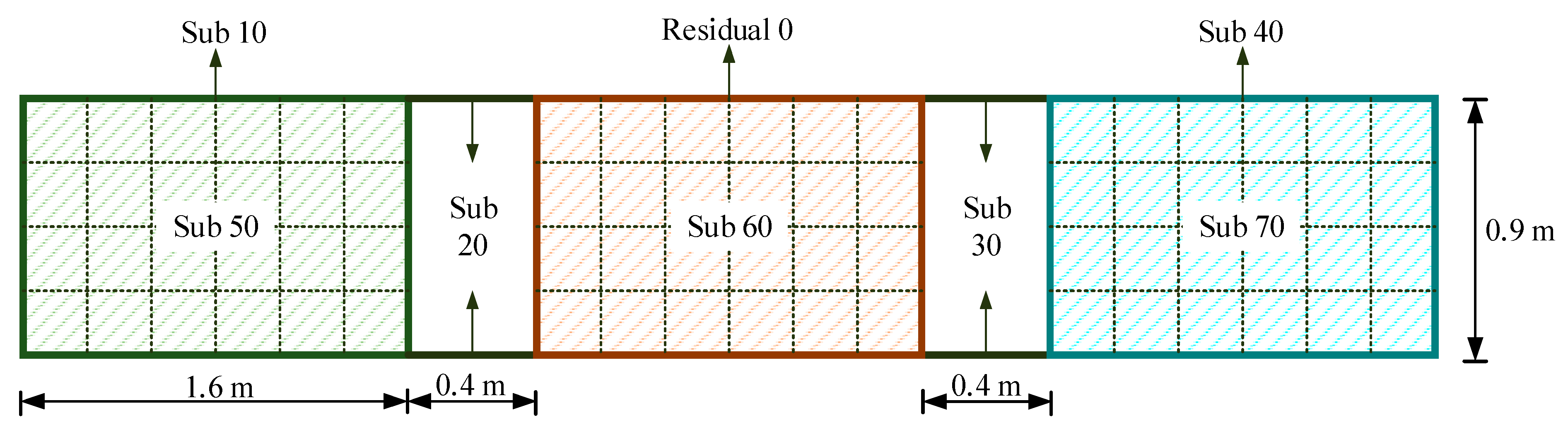
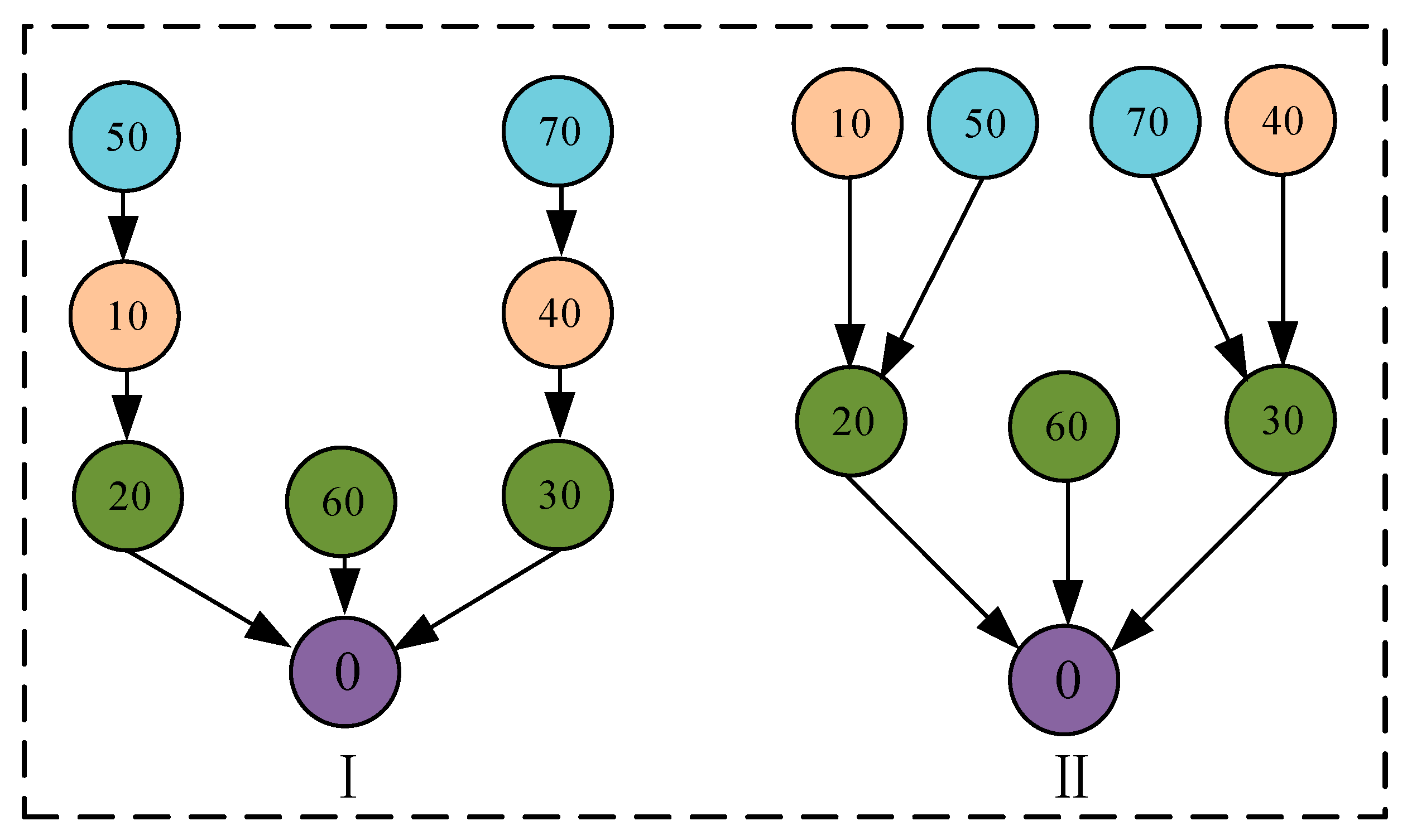
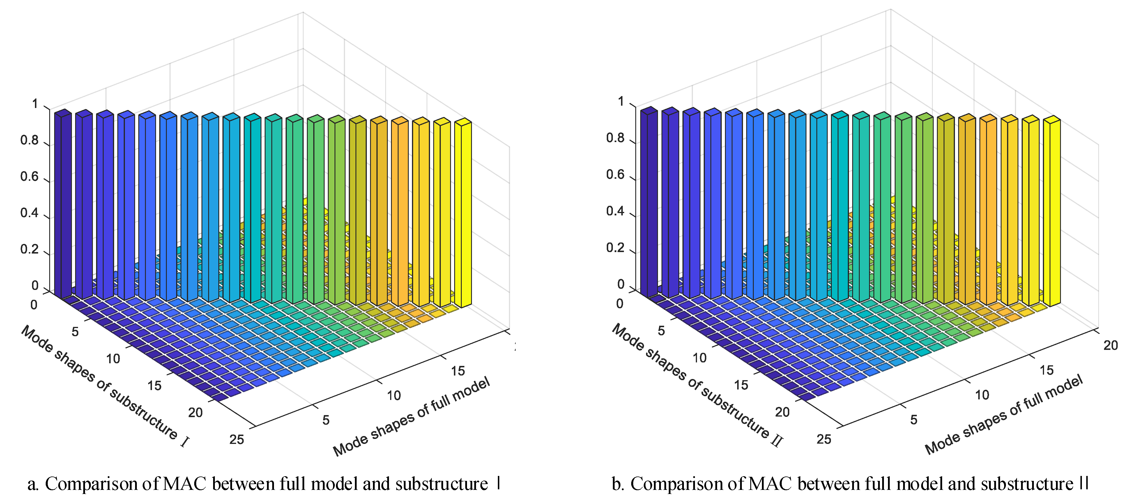
4.1. Assembly Structure with Three Panels

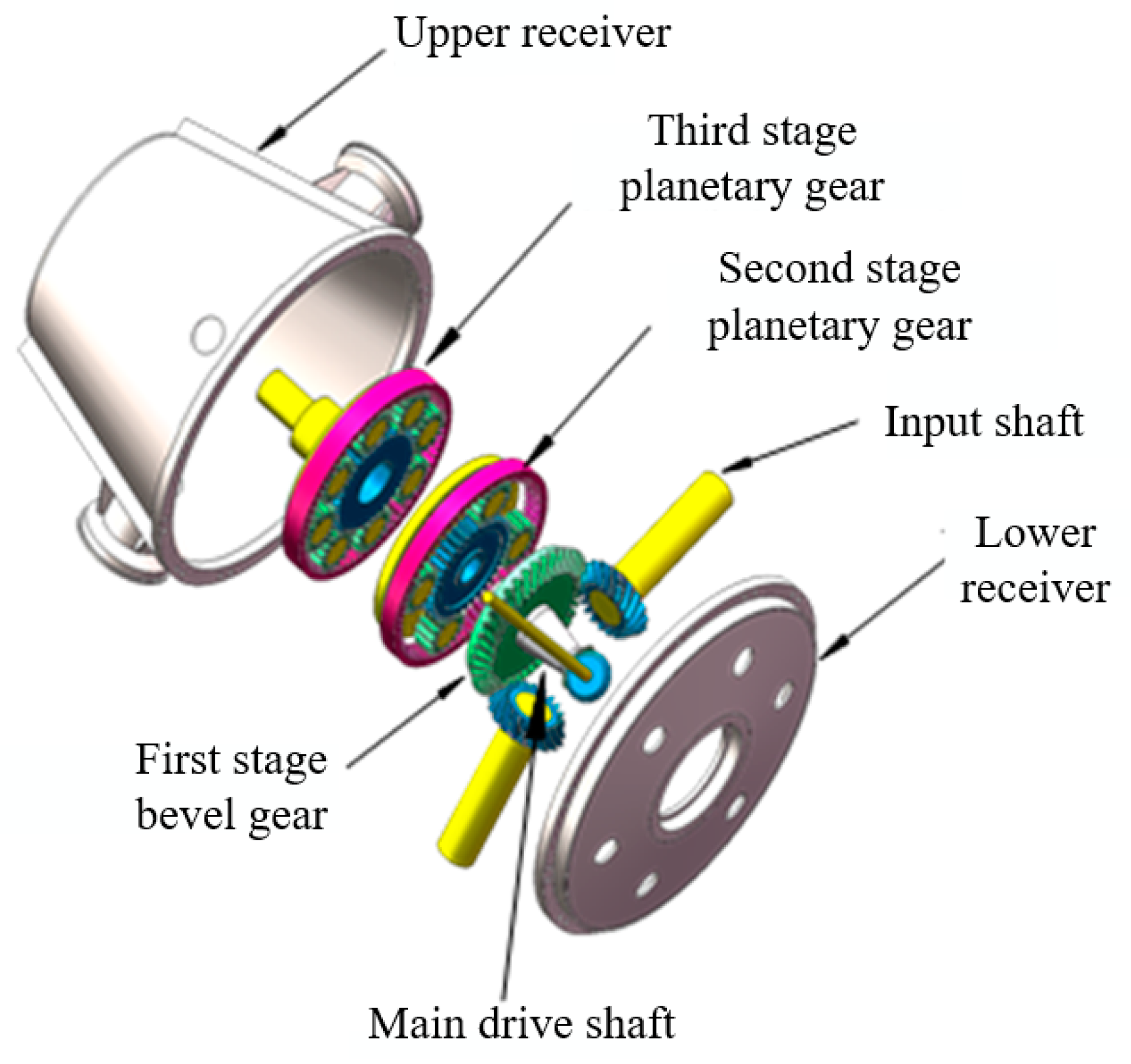
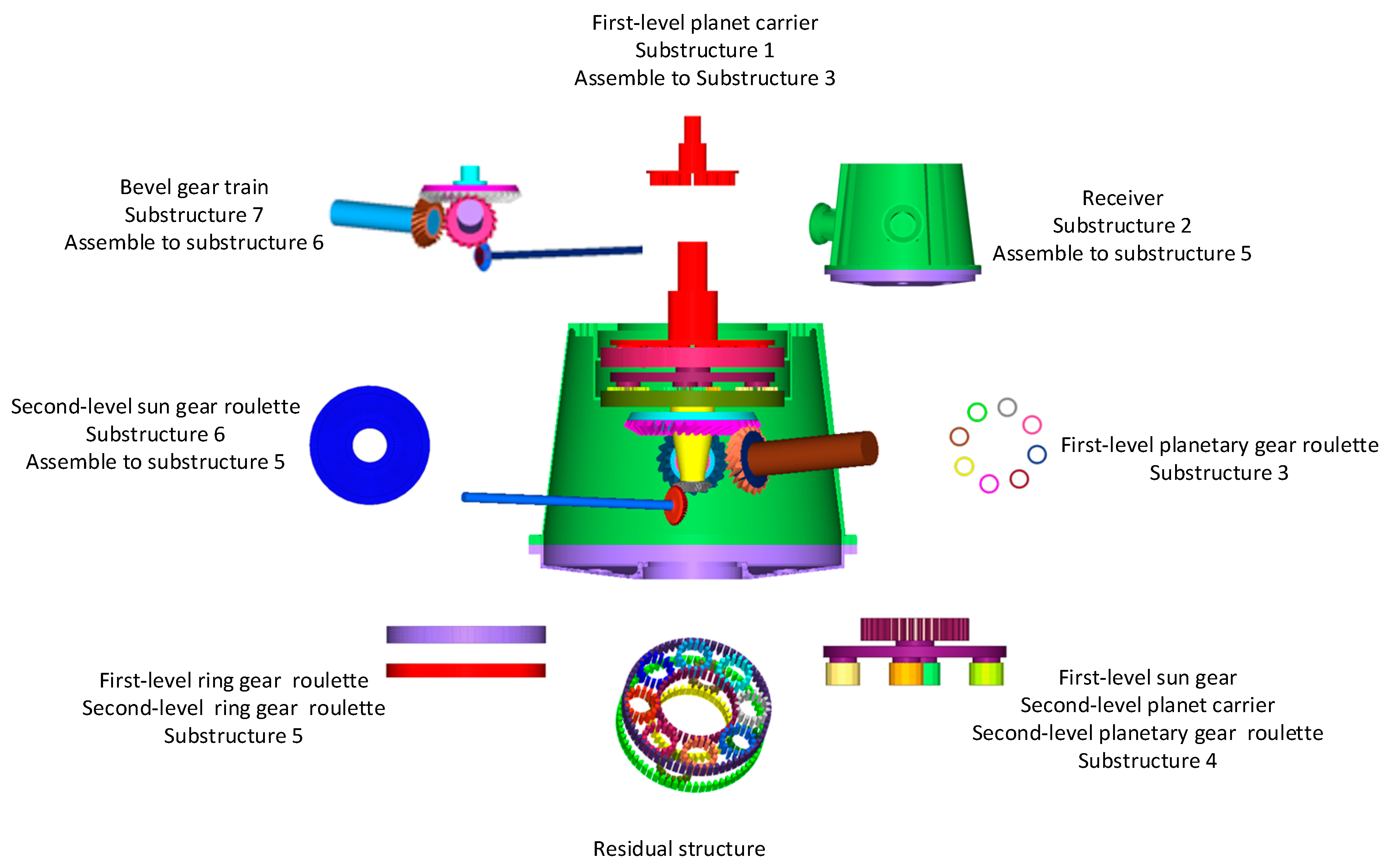
The research object of this example is the assembly structure with three panels. A complete FE model of the assembly structure with three panels was modeled by the FE analysis software ‘Nastran’ and ‘Hypermesh’ based on the size diagram of the assembly structure with three panels, as shown in Figure 2. The assembly structure with three panels is a top and bottom axisymmetric structure, composed of three plates of the same material and the same geometric shape [31]. The finite element model is composed of shell elements and beam elements. The periphery of the slab is surrounded by beam elements, and the slab is connected by beam elements. A total of 12,397 nodes and 12,784 elements were established by using ‘Hypermesh’. Among them, the shell element has 12,397 nodes and 12,000 elements, and the beam element has 780 nodes and 784 elements. All the nodes are hinged. The beam element is steel and the cross-sectional area of the beam is A₁ = 4 × 10⁻⁴ m². The shell element is an aluminum alloy and the thickness is t = 4 × 10⁻³ m. Our assumption is a homogeneous, isotropic, linearly elastic material. The material and its parameters of the finite element model are as they are shown in

Table 1. Material parameters of the assembly structure with three panels.

Type of Element	Material	Elastic Modulus/GPa	Density/g·cm−3	Poisson’s Ratio
Shell element “50”	aluminum	70	2.7	0.34
Shell element “60”	aluminum	70	2.7	0.34
Shell element “70”	aluminum	70	2.7	0.34
Beam element	steel	200	7.85	0.32

.

There are two substructure classifications for the assembly structure with three panels. The specific classification is shown in Figure 3. For the analysis of the substructure, we selected the first 20 order models for free mode analysis (it mainly studies the improvement of the efficiency of modal calculation, so it is only carried out at a normal temperature). The first 20 natural frequencies are as they are shown in

Table 2. Natural frequency error analysis of full model and multi-level substructure model.

Order	Natural Frequency/Hz			Error/%
	Full Model	Substructure III	Substructure IV	Comparison of Full Model and Substructure III	Comparison of Full Model and Substructure IV
1	1.89100	1.89096	1.89101	0.00212	0.00053
2	4.53726	4.53703	4.53727	0.00507	0.00022
3	5.16572	5.16559	5.16574	0.00252	0.00039
4	9.28268	9.28217	9.28273	0.00549	0.00054
5	10.18671	10.18639	10.18682	0.00314	0.00108
6	14.15608	14.15563	14.15698	0.00318	0.00636
7	16.41321	16.40970	16.41343	0.02138	0.00134
8	20.95025	20.94964	20.95272	0.00291	0.01180
9	23.28714	23.27322	23.28847	0.05978	0.00571
10	28.77556	28.78435	28.77634	0.03055	0.00271
11	29.34067	29.30249	29.34342	0.13013	0.00937
12	32.17115	32.15329	32.17310	0.05552	0.00606
13	33.11550	33.07276	33.11612	0.12906	0.00187
14	33.87447	33.83622	33.87468	0.11292	0.00062
15	38.41049	38.45056	38.42395	0.10432	0.03504
16	39.01908	38.95087	39.02331	0.17481	0.01084
17	41.12772	41.05179	41.13019	0.18462	0.00601
18	42.52401	42.51023	42.71097	0.03241	0.43966
19	47.04580	46.98833	47.05776	0.12216	0.02542
20	49.23641	49.18840	49.24422	0.09751	0.01586

. Analyzing the natural frequency error of Table 2, we can see that the maximum error occurs in the seventeenth and eighteenth steps, respectively, which are 0.18462% and 0.43966%, indicating that different classification methods do not affect the calculation accuracy. The modal assurance criteria (MAC) is used to verify the modal. The comparison of MAC between the full model and the substructure model is shown in Figure 4. The diagonal element of the MAC is 1, and the rest is close to 0, which indicates that the modal shapes are consistent.

Further considering the influence of the selection of external nodes in the substructure model on the analysis results, 25%, 50%, and 75% of external nodes are selected for calculation and free mode analysis. The natural frequency error curve is shown in Figure 5. The maximum absolute value errors of the corresponding frequencies are 0.255%, 0.077%, and 0.026%, respectively. The comparison shows that the calculation accuracy of the substructure model is improved with the increase of the number of external nodes, that is, the calculation accuracy is related to the number of selected external nodes of the substructure.

Table 3. Time-consuming of analysis for assembly structure with three panels model with different numbers of nodes.

	25% Nodes	50% Nodes	75% Nodes	100% Nodes
Analysis time/s	21.871	27.919	35.598	48.427

shows the analysis time of the substructure models with the different number of nodes, and the analysis time of the substructure model rises with the increase in the number of external nodes. Considering the benefits comprehensively, selecting 50% external nodes can further improve the calculation efficiency while ensuring the accuracy.

In order to consider the influence of the selection of the residual structure on the analysis results, the residual structure is changed from the number “0” in Figure 3 to the number “60”, and the specific classification methods are shown in Figure 6.

The free mode analysis of the model shown in Figure 6 is established, and the results are shown in

Table 4. Frequency of substructure I and II for the assembly structure with three panels.

Order	Natural Frequency/Hz			Error/%
	Full Model	Substructure I	Substructure II	Comparison of Full Model and Substructure I	Comparison of Full Model and Substructure II
1	1.89100	1.89105	1.89093	0.00264	0.00370
2	4.53726	4.53723	4.53851	0.00066	0.02755
3	5.16572	5.16579	5.17013	0.00135	0.08537
4	9.28268	9.28284	9.28297	0.00172	0.00312
5	10.18671	10.18677	10.18726	0.00059	0.00540
6	14.15608	14.16634	14.14894	0.07248	0.05044
7	16.41321	16.41983	16.41348	0.04016	0.00165
8	20.95025	20.95247	20.95397	0.01060	0.01776
9	23.28714	23.28816	23.28967	0.00438	0.01086
10	28.77556	28.77670	28.77638	0.00396	0.00285
11	29.34067	29.30272	29.34351	0.12934	0.00968
12	32.17115	32.15182	32.16689	0.06008	0.01324
13	33.11550	33.08684	33.11634	0.08655	0.00254
14	33.87447	33.81954	33.87451	0.16215	0.00012
15	38.41049	38.15891	38.42406	0.65498	0.03533
16	39.01908	39.00173	39.02286	0.04447	0.00969
17	41.12772	41.05358	41.13100	0.18028	0.00796
18	42.52401	42.52094	42.71124	0.00722	0.44029
19	47.04580	47.00132	47.04365	0.09455	0.36974
20	49.23641	49.16967	49.24467	0.13555	0.01678

. Selection of the residual structure has no effect on the dynamic modeling and analysis results of the assembly structure with a three panel substructure, indicating that the selection of the residual structure is not unique.

4.2. Gear Box

The object of this example is the gear box of a helicopter, which is composed of a three-level planetary gear train and a receiver. The first-level planetary gear train is to change the direction of the power input by the engine through the bevel gear train to reduce the speed, and to complete the output to the tail rotor. The output deceleration power is input to the tail rotor reducer through the horizontal tail drive and the inclined tail drive shaft. The tail rotor reducer realizes the power conversion of the tail wing. The second-level planetary gear train uses the output power of the bevel gear train in the first-level planetary gear train as the input power of the second-level reducer. After planetary gear reduction, the planet carrier realizes the power output. The third-level planetary gear system uses the output power of the planet carrier in the second-level planetary gear system as the output power of the third-level reducer. After the transmission of the planetary gear system, the output of the planet carrier is completed, and the decelerated power can be passed to the helicopter rotor. Figure 7 shows the exploded view of the geometric model of the whole machine.

The material of the gear box is steel. Our assumption is homogeneous, isotropic, linearly elastic material. The elastic modulus is 190 GPa, the Poisson’s ratio is 0.3, and the density is 7.75 g/cm³. The whole structure is modeled by ‘Hypermesh’ with tetrahedral and hexahedral meshes. The finite element model has a total of 1,220,562 nodes and 1,111,039 elements. The receiver has 298,047 nodes and 303,696 elements. The multi-level planetary gear train has 924,789 nodes and 807,343 elements.

Based on the analysis in Section 4.1, the planetary gear train teeth in the gear box is selected as the residual structure, 50% of the external nodes is selected, then the whole structure is divided into multiple and multi-level substructures which are shown in Figure 8. Free mode analysis is performed on the substructure model and the finite element model, respectively. The first five-order modal shapes and natural frequencies are selected for comparison.

Table 5. Modal shapes of the finite element model for the whole structure.

Order	Mode 1	Mode 2	Mode 3	Mode 4	Mode 5
Mode shape of FEM

shows the modal shapes of the gear box. Analyzing the natural frequency error of

Table 6. Frequency error analysis of finite element model and substructure model.

Order	Natural Frequency/Hz		Error/%
	Finite Element Model	Substructure Model
1	47.23	47.60	0.7686
2	48.75	48.80	0.1075
3	94.05	92.70	1.4333
4	102.59	101.99	0.5843
5	121.35	120.23	0.9231

, the maximum error of the model appears in the third order, which is 1.4333%. The frequency errors of the other fourth orders are all less than 1%, and the calculation deviation is small. Through the comparison of the time-consuming analysis of dynamic characteristics in

Table 7. Comparison of calculation time-consuming between finite element model and substructure model.

Time-Consuming of Finite Element Model/s	Time-Consuming of Substructure Model/s	Δt/s	The Ratio of Reduction/%
15062	5364	9698	64.39

, the analysis of the inherent characteristics of the multi-level substructure model takes 5364 s. Compared with the finite element model, the multi-level substructure model saves 9698 s. The comparison of MAC between the full model and the substructure model is shown in Figure 9. The diagonal element of the MAC is 1, and the rest is close to 0, which in-dicates that the modal shapes are consistent.

4.3. Modal Experiment of Combustion Rotor and Verification of Substructure Method

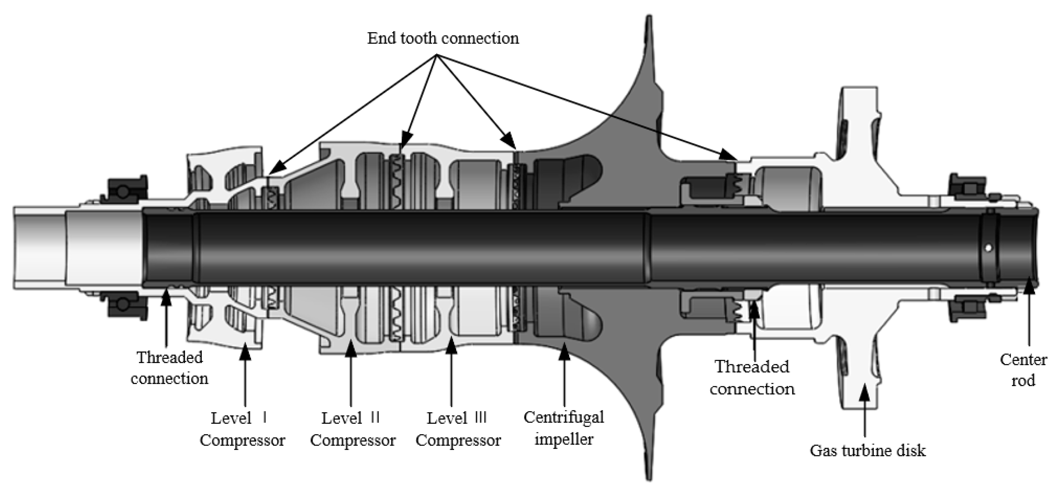
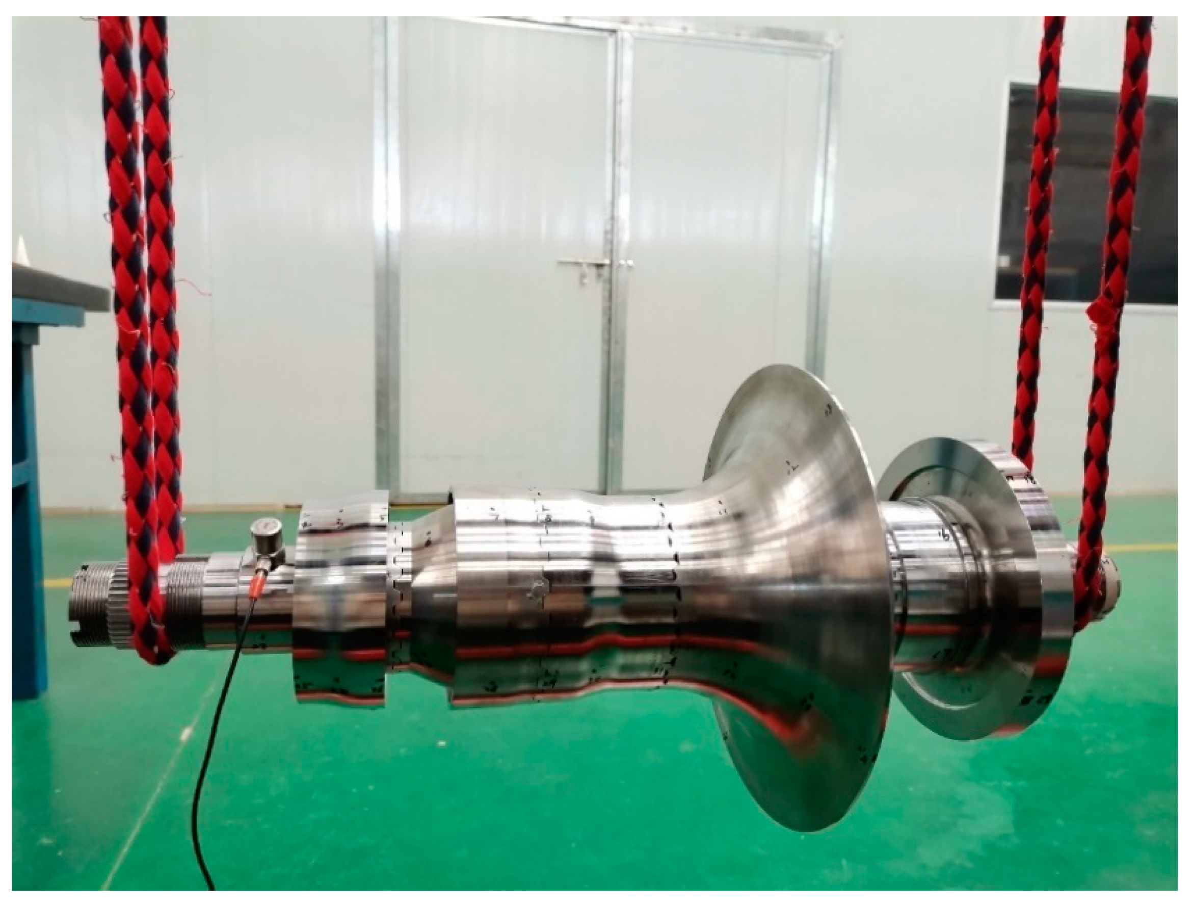
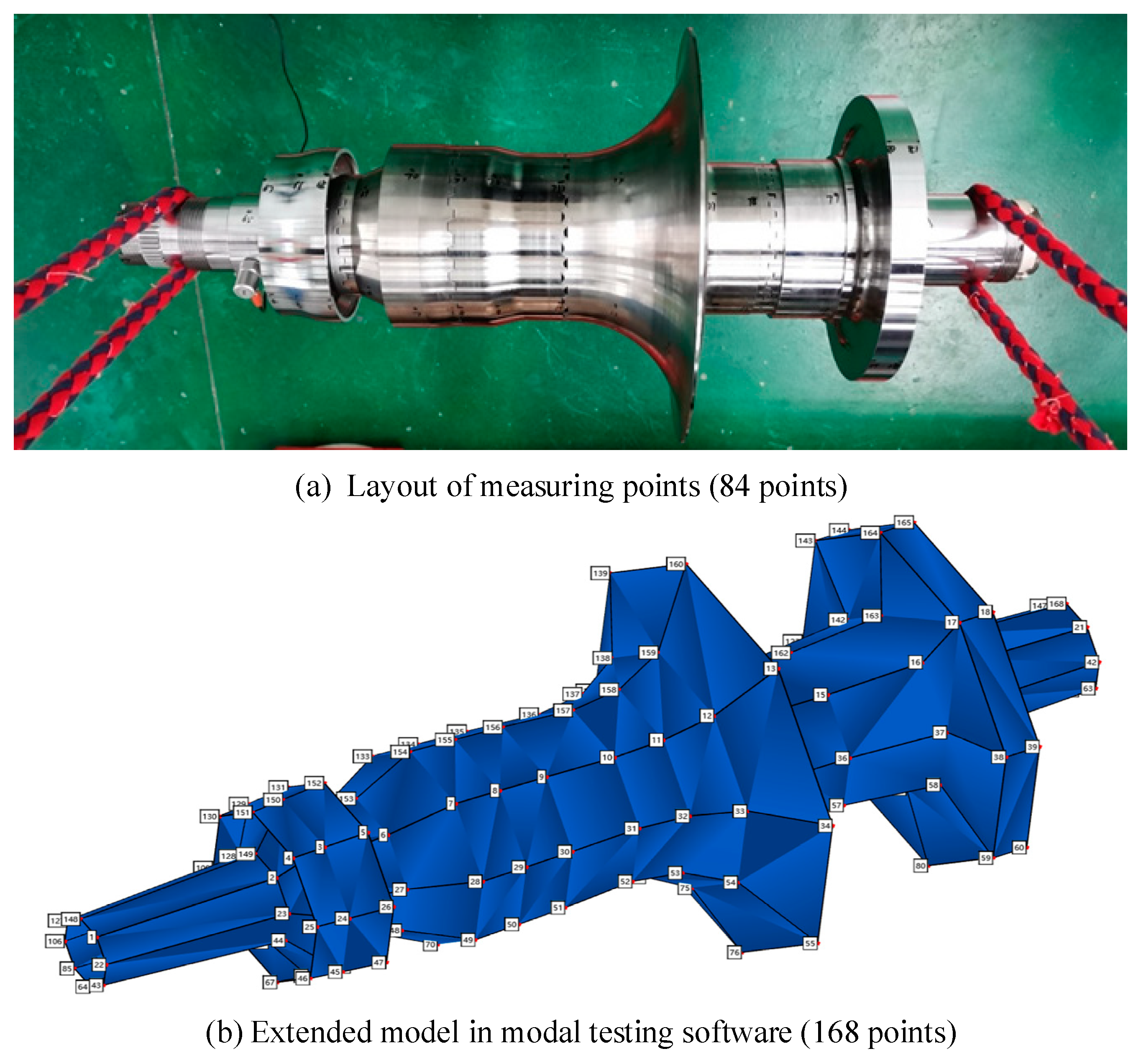
4.3.1. Object of the Experiment

In this experiment, a free-modal experiment is carried out for the combustion rotor of an engine shown in Figure 10. The combustion rotor is pre-tightened in sections, with a pre-tightening force of 9.8 t at the front section and 6.8 t at the rear section.

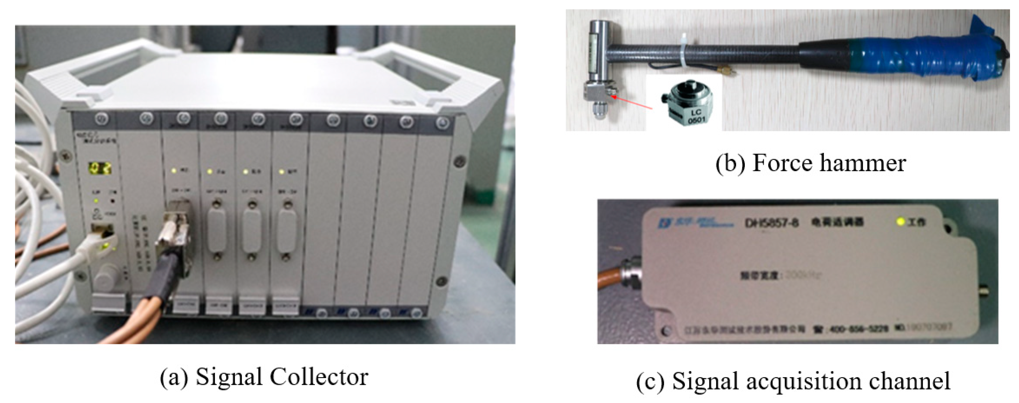
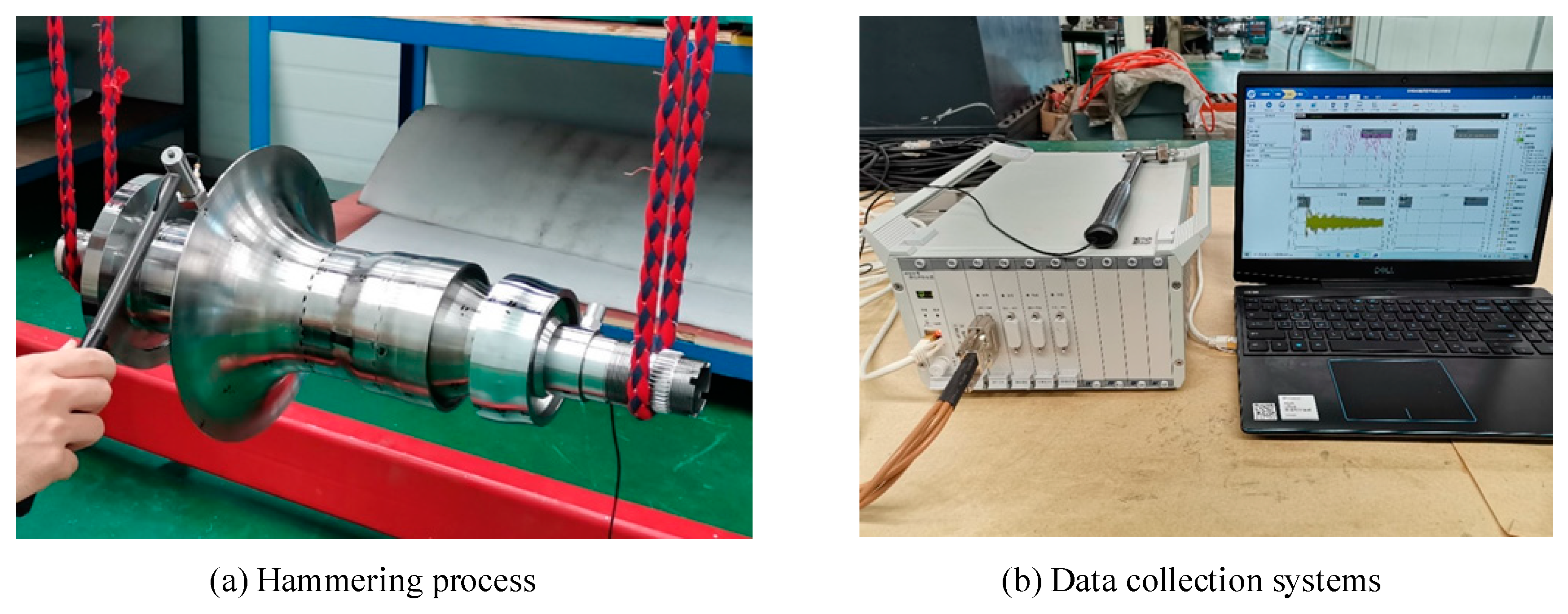
4.3.2. Experiment System

Experimental modal analysis methods can be divided into a frequency response function method and environmental excitation method. The so-called force measurement method is a method that needs to measure the excitation force and response at the same time during the experiment. The classic force measurement method uses the frequency response function (FRF) in the frequency domain or the impulse response function (IRF) in the time domain to estimate the modal parameters. The frequency response function is the ratio of the Fourier transform of the response and the force, and the impulse response function must be measured first and then obtained by the inverse Fourier transform. Therefore, the force measurement method must use a vibrator or a hammer with a dynamometer to apply a measurable excitation force. The force measurement method can estimate all modal parameters, including natural frequency, modal shape, damping or damping ratio, modal mass and modal stiffness; furthermore, the accuracy is high.

a. Boundary conditions

This experiment is a free-mode experiment of the combustion rotor. In order to avoid other structures or excitation sources from affecting the test results, the installation method selected this time is the free suspension method. This installation method can eliminate external interference to the greatest extent and ensure the accuracy of the test results. The suspension mode is shown in Figure 11.

b. Incentive method and acquisition system

Modal test experiments can be divided into a hammering method and a vibration exciter method [32]. The hammering method is generally suitable for cases where the mass and the volume of the test piece is small, and its characteristic is that the test is convenient; the vibration exciter method is generally suitable for the case of the large mass and volume of the test object, and its advantage is that a larger excitation can be generated by the vibration exciter to stimulate the inherent characteristics of the test object. The research object of this experiment is the combustion-engine rotor. According to the above description, the free modal experiments are carried out by the hammering method of multi-point excitation and a single-point vibration pickup. The modal experiment equipment used in this experiment is the Donghua DHDAS dynamic signal acquisition and analysis system shown in Figure 12. The model is DH5922D, which is used to collect force signals and acceleration signals. Channel 1 is connected to the force hammer, and channel 2 is connected to the acceleration sensor. The head of the force hammer is rubber, the sensitivity of the force sensor is 3.65 mV/N; the acceleration sensor can convert the acceleration of mechanical vibration into an electric charge to output, whose sensitivity is 2.86 mV/m/s². The starting point of tapping is the No. 1 measuring point, tapping in the order of the number of the measuring points, tapping twice for each measuring point, and linearly averaging the results collected by tapping, and then obtaining the tapping data of the measuring point. In the process of percussion, you need to pay attention to the intensity of the percussion. If the intensity is too large, it is easy to cause an overload. If the intensity is too small, the data cannot be collected. In addition, it is necessary to be quick and accurate in the process of percussion to prevent the occurrence of combos, which will affect the results.

c. Layout of measuring points

The experiment mainly uses the hammer method to measure the natural frequency and vibration mode of the combustion rotor. Firstly, the ignition rotor is divided into 84 points. The sensor is located at No. 2 point. As shown in Figure 13a, each bus has 21 points, and 84 points of 4 bus are measured altogether. Secondly, the cylindrical coordinates are used in the DHDAS software to carry out modeling and to extend to 168 points of 8 busbars, as shown in Figure 13b. The model required for modal analysis can be obtained by inputting the coordinates of the measuring points and connecting the points together to form a plane. Finally, according to this model, the test pieces are marked with measuring points. For eight points on the cylinder surface in a week, only four points on the plane coordinate axis are needed to measure, and the remaining four points can be combined proportioning through two adjacent measuring points.

4.3.3. Data Acquisition

Data collection is divided into two steps: preparation for collection and formal collection. On the one hand, preparation for collection is to determine reasonable parameters, such as sampling frequency, acquisition range, sampling duration, excitation signal, reference point, etc. On the other hand, data need to be checked, including a linearity check, FRF, coherence check, reciprocity check and so on. Collections begin after calibration. Once a set of data have been formally collected, the consistency of the measured data should be checked in both the time and frequency domains.

The connected data acquisition instrument and the computer, as well as the hammer and sensors, were as shown in Figure 14. Before measurement, relevant parameters of the software were set, and the highest frequency of the first three modes of concern was about 4 kHz after preliminary simulation. Therefore, the analysis frequency in the setting was 5 kHz, and the sampling frequency was 12.8 kHz.

In the test process, attention should be paid to the time domain diagram and the corresponding spectrum diagram of the excitation signal. This experiment uses the hammering method, and the signal should be as smooth as possible to extend to the specified frequency. In addition, in the modal experiment, the coherence function is used to describe the linear relationship of multiple measured data. Its value range is 0~1. The coherence function is equal to 1, which means the data has a good linear relationship. If the coherence value is low, the data may be affected by noise or leakage, resulting in large differences between the data. The coherence value is generally required to be greater than 0.8 in the experiment.

4.3.4. Identification of a Modal Parameter

This part is to use the measured frequency response function or time history to estimate the modal parameters, including natural frequency, modal shape, modal damping, modal stiffness and modal mass. The essence of modal analysis is the process of curve fitting. According to the measured data (frequency response function, FRF), the modal parameters are obtained through curve fitting. After obtaining the modal parameters of each order, the FRF of each measuring point can be synthesized based on these parameters. The curve fitting is divided into single degree-of-freedom fitting and multi-degree-of-freedom fitting, local fitting and overall fitting.

Polylscf is a newly developed and popular modal analysis method based on transfer function. In the case of the system with relatively dense modes or the FRF data polluted seriously by noise, a clear steady state diagram can still be established to identify the highly dense modes, and a good identification accuracy can be obtained for the frequency, damping and shape of each mode.

Table 8. Free-mode experimental results of the combustion rotor (three-dimensional).

Order	Modal Shape	Modal Frequency/Hz	Damping Ratio/%
1		1254.9 Hz	0.166
2		2525.2 Hz	0.216
3		3584.7 Hz	0.067

shows the 3D modal shapes, frequencies and damping ratios finally obtained through the modal experiment.

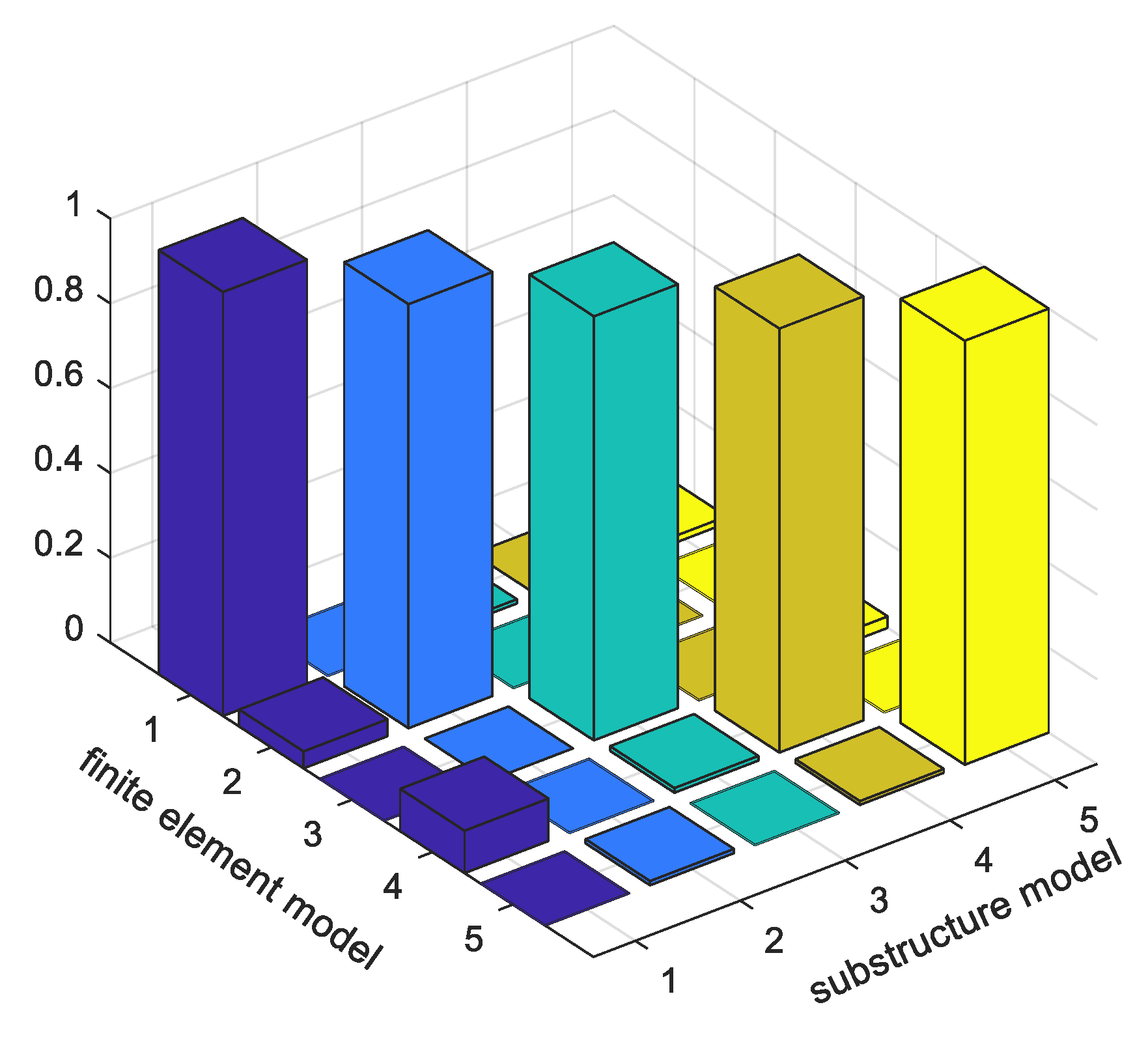
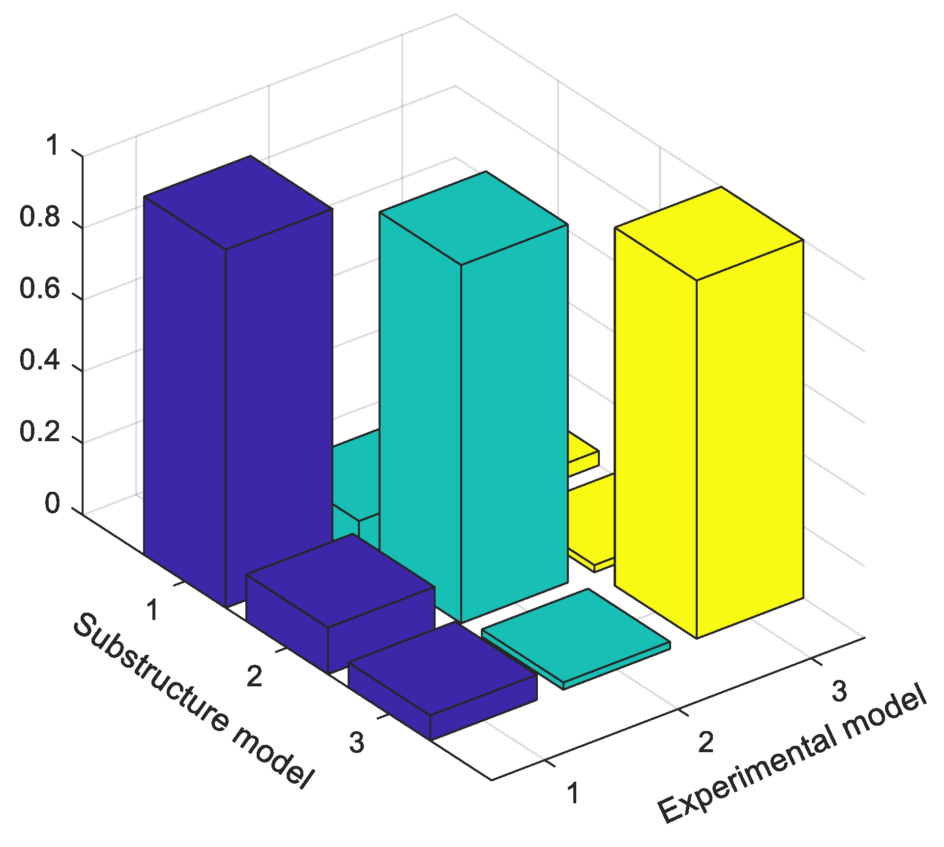
4.3.5. Verification of Substructure Method

The tetrahedral and hexahedral meshes are used to model the combustion rotor. The finite element model has 16,530 nodes and 10,980 elements in total. Our assumption is a homogeneous, isotropic, linearly elastic material. The material parameters are shown in

Table 9. Material parameters of a combustion rotor.

Material	Elastic Modulus/GPa	Density/g·cm−3	Poisson’s Ratio
Steel	196	7.8	0.3
Titanium alloy	121	4.48	0.3
Nickel base alloy	204	8.24	0.3
Nickel base alloy	214	8.3	0.3

.

Based on the analysis in Section 4.1, the center rod of the combustion rotor is selected as the residual structure, and 50% of the external nodes are selected, and then the substructure is divided. The finite element model and substructure division method of the combustion rotor are shown in Figure 15. Free mode analysis is performed on the substructure model and the finite element model, respectively. The first three-order modal shapes and natural frequencies are selected for comparison. From

Table 10. Frequency and error of each model.

Order	Natural Frequency/Hz		Error/%
	Experimental Model	Sub	Experimental Model and Sub
1	1254.9	1335.7	6.4
2	2525.2	2396.3	−5.1
3	3584.7	3816.4	6.5

, it can be seen that the calculation deviation is small. According to the time-consuming comparison of the dynamic characteristic analysis in

Table 11. Model calculation time-consuming of the combustion rotor.

	Finite Element Model	Substructure Model	Δt	The Ratio of Reduction/%
Time-consuming/s	47.15	22.78	24.37	51.69

, the multi-level substructure model saves 24.37 s compared with the finite element model. Figure 16 is the diagram of modal assurance criteria. The diagonal element of the MAC is 1, and the rest is close to 0, which indicates that the modal shapes are consistent.

5. Conclusions

The substructure method can effectively reduce the degree of freedom of the complex and huge multi-degree of freedom system, and then improve the analysis efficiency. In this paper, based on the fixed interface modal synthesis method, the dynamic characteristics analysis based on the multi-level substructure and the full model finite element analysis of the assembly structure with three panels, gear box of a helicopter and combustion rotor are carried out. The method is simple and feasible, and has an engineering application value. The following conclusions are drawn:

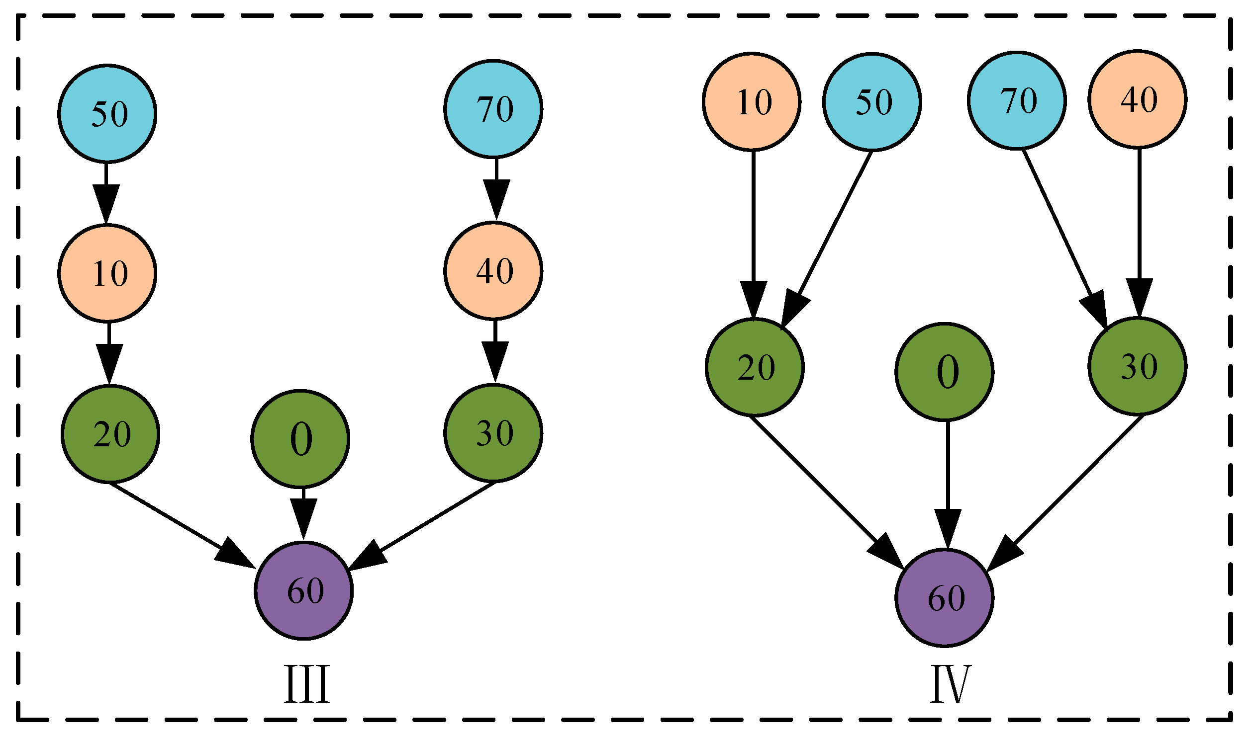
• In the substructure calculation and analysis of actual engineering structures, the selection of residual structures is not unique;
• For the same residual structure, the calculation accuracy of the substructure will not be affected by different substructure division methods, and the high-precision dynamic characteristic analysis can be realized;
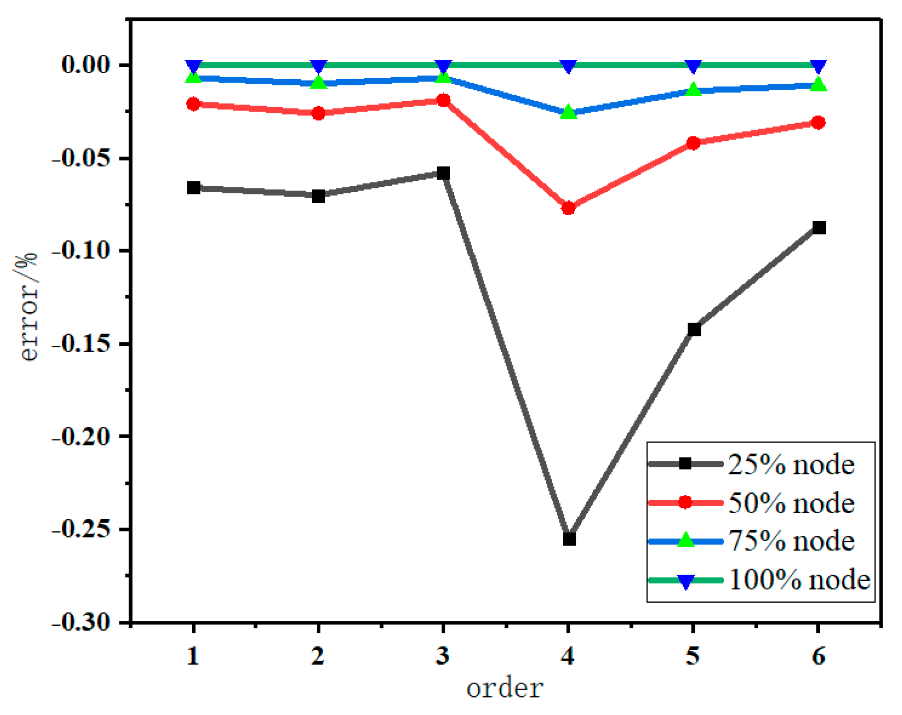
• The modal frequency accuracy of the substructure model is related to the number of selected external nodes of the substructure. On the premise of ensuring accuracy, the selection of 50% external nodes can further improve the computational efficiency.

References

1. Weng, S.; Xia, Y.; Xu, Y.-L.; Zhou, X.-Q.; Zhu, H.-P. Improved substructuring method for eigensolutions of large-scale structures. J. Sound Vib. 2009, 323, 718–736. [Google Scholar] [CrossRef] [Green Version]
2. Liu, J.; Fei, Q.; Jiang, D.; Zhang, D.; Wu, S. Experimental and numerical investigation on static and dynamic characteristics for curvilinearly stiffened plates using DST–BK model. Int. J. Mech. Sci. 2020, 169, 105286. [Google Scholar] [CrossRef]
3. Gu, Y. Mode-dependent phonon transmission in a T-shaped three-terminal graphene nanojunction. Carbon 2020, 158, 818–826. [Google Scholar] [CrossRef]
4. Zhou, J.; Xu, L.; Liu, G.; Xuan, Y.; Zhou, H.; Jiang, H. Frequency Response Curves and Dynamic Characteristics of a Ginkgo Tree in Different Growth Periods. Trans. ASABE 2020, 63, 1673–1684. [Google Scholar] [CrossRef]
5. Torabi, J.; Ansari, R. A higher-order isoparametric superelement for free vibration analysis of functionally graded shells of revolution. Thin-Walled Struct. 2018, 133, 169–179. [Google Scholar] [CrossRef]
6. Zhang, D.; Fei, Q.; Liu, J.; Jiang, D.; Li, Y. Crushing of vertex-based hierarchical honeycombs with triangular substructures. Thin-Walled Struct. 2020, 146, 106436. [Google Scholar] [CrossRef]
7. Bai, B.; Bai, G.-C. Dynamic probabilistic analysis of stress and deformation for bladed disk assemblies of aeroengine. J. Central South Univ. 2014, 21, 3722–3735. [Google Scholar] [CrossRef]
8. Bai, B.; Bai, G.C.; Li, C. Application of multi-stage multi-objective multi-disciplinary agent model based on dynamic substructural method in Mistuned Blisk. Aerosp. Sci. Technol. 2015, 46, 104–115. [Google Scholar] [CrossRef]
9. Bai, B.; Li, H.; Zhang, W.; Cui, Y. Application of extremum response surface method-based improved substructure component mode synthesis in mistuned turbine bladed disk. J. Sound Vib. 2020, 472, 115210. [Google Scholar] [CrossRef]
10. Gu Y, F. An efficient Laplace transform-wave packet method hybrid with substructure technique. Comput. Mater. Sci. 2015, 110, 345–352. [Google Scholar] [CrossRef]
11. Duan, Y.; Zang, C.; Petrov, E.P. Forced Response Analysis of High-Mode Vibrations for Mistuned Bladed Disks With Effective Reduced-Order Models. J. Eng. Gas Turbines Power 2016, 138, 112502. [Google Scholar] [CrossRef] [Green Version]
12. Jung, C.; Saito, A.; Epureanu, B.I. Detection of Cracks in Mistimed Bladed Disks Using Reduced-Order Models and Vibration Data. J. Vib. Acoust. 2012, 134, 061010. [Google Scholar] [CrossRef]
13. Zhu, H.; Li, J.; Tian, W.; Weng, S.; Peng, Y.; Zhang, Z.; Chen, Z. An enhanced substructure-based response sensitivity method for finite element model updating of large-scale structures. Mech. Syst. Signal Process. 2021, 154, 107359. [Google Scholar] [CrossRef]
14. Tian, W.; Weng, S.; Xia, Y.; Zhu, H.; Gao, F.; Sun, Y.; Li, J. An iterative reduced-order substructuring approach to the calculation of eigensolutions and eigensensitivities. Mech. Syst. Signal Process. 2019, 130, 361–377. [Google Scholar] [CrossRef]
15. Weng, S.; Xia, Y.; Xu, Y.L.; Zhu, H. An iterative substructuring approach to the calculation of eigensolution and eigensensitivity. J. Sound Vib. 2011, 330, 3368–3380. [Google Scholar] [CrossRef]
16. Weng, S.; Zhu, H.-P.; Xia, Y.; Zhou, X.-Q.; Mao, L. Substructuring approach to the calculation of higher-order eigensensitivity. Comput. Struct. 2013, 117, 23–33. [Google Scholar] [CrossRef] [Green Version]
17. Weng, S.; Xia, Y.; Xu, Y.-L.; Zhu, H.-P. Substructure based approach to finite element model updating. Comput. Struct. 2011, 89, 772–782. [Google Scholar] [CrossRef] [Green Version]
18. Jiang, D.; Zhang, P.; Fei, Q.; Wu, S. Comparative study of model updating methods using frequency response function data. J. Vibroeng. 2014, 16, 2305–2318. [Google Scholar]
19. Shamloofard, M.; Hosseinzadeh, A.; Movahhedy, M.R. Development of a shell superelement for large deformation and free vibration analysis of composite spherical shells. Eng. Comput. 2020, 1–17. [Google Scholar] [CrossRef]
20. Fatan, A.; Ahmadian, M. Vibration analysis of FGM rings using a newly designed cylindrical superelement. Sci. Iran. 2017, 25, 1179–1188. [Google Scholar] [CrossRef] [Green Version]
21. Plaza, J.; Abasolo, M.; Coria, I.; Aguirrebeitia, J.; De Bustos, I.F. A new finite element approach for the analysis of slewing bearings in wind turbine generators using superelement techniques. Meccanica 2015, 50, 1623–1633. [Google Scholar] [CrossRef]
22. Tuysuz, O.; Altintas, Y. Frequency Domain Updating of Thin-Walled Workpiece Dynamics Using Reduced Order Substructuring Method in Machining. J. Manuf. Sci. Eng. 2017, 139, 071013. [Google Scholar] [CrossRef]
23. Tuysuz, O.; Altintas, Y. Time-Domain Modeling of Varying Dynamic Characteristics in Thin-Wall Machining Using Perturbation and Reduced-Order Substructuring Methods. J. Manuf. Sci. Eng. 2017, 140, 011015. [Google Scholar] [CrossRef]
24. Cao, Z.F.; Fei, Q.G.; Jiang, D.; Wu, S. Substructure-based model updating using residual flexibility mixed-boundary method. J. Mech. Sci. Technol. 2017, 31, 759–769. [Google Scholar] [CrossRef]
25. Hang, X.; Su, W.; Fei, Q.; Jiang, D. Analytical sensitivity analysis of flexible aircraft with the unsteady vortex-lattice aerodynamic theory. Aerosp. Sci. Technol. 2020, 99, 105612. [Google Scholar] [CrossRef]
26. Zhu, R.; Fei, Q.; Jiang, N.; Cao, Z. Maintaining Specific Natural Frequency of Damped System despite Mass Modification. Int. J. Aerosp. Eng. 2019, 2019, 1–11. [Google Scholar] [CrossRef]
27. Géradin, M.; Rixen, D. A ‘nodeless’ dual superelement formulation for structural and multibody dynamics application to reduction of contact problems. Int. J. Numer. Methods Eng. 2015, 106, 773–798. [Google Scholar] [CrossRef]
28. Voormeeren, S.N.; Van Der Valk, P.L.C.; Nortier, B.P.; Molenaar, D.-P.; Rixen, D. Accurate and efficient modeling of complex offshore wind turbine support structures using augmented superelements. Wind. Energy 2014, 17, 1035–1054. [Google Scholar] [CrossRef]
29. Cui, J.; Guan, X.; Zheng, G. A simultaneous iterative procedure for the Kron’s component modal synthesis approach. Int. J. Numer. Methods Eng. 2015, 105, 990–1013. [Google Scholar] [CrossRef]
30. Cui, J.; Wang, X.; Xing, J.; Zheng, G. An eigenvector-based iterative procedure for the free-interface component modal synthesis method. Int. J. Numer. Methods Eng. 2018, 116, 723–740. [Google Scholar] [CrossRef]
31. Wu, Y.; Zhu, R.; Cao, Z.; Liu, Y.; Jiang, D. Model Updating Using Frequency Response Functions Based on Sherman–Morrison Formula. Appl. Sci. 2020, 10, 4985. [Google Scholar] [CrossRef]
32. Zhu, R.; Fei, Q.-G.; Jiang, D.; Cao, Z.-F. Removing mass loading effects of multi-transducers using Sherman-Morrison-Woodbury formula in modal test. Aerosp. Sci. Technol. 2019, 93, 105241. [Google Scholar] [CrossRef]
Figure 1. Schematic diagram of multiple and multi-level substructure.
Applsci 11 05570 g001
Figure 2. Finite element model of the assembly structure with three panels.
Applsci 11 05570 g002
Figure 3. Different classification of substructure for the assembly structure with three panels.
Applsci 11 05570 g003
Figure 4. Comparison of MAC between full model and substructure model.
Applsci 11 05570 g004
Figure 5. Frequency error curves of the substructure model with different number of nodes.
Applsci 11 05570 g005
Figure 6. Substructure model I and II for the assembly structure with three panels.
Applsci 11 05570 g006
Figure 7. Explosion diagram of the gear box.
Applsci 11 05570 g007
Figure 8. Substructure model of the gear box.
Applsci 11 05570 g008
Figure 9. Comparison of MAC between finite element model and the substructure model.
Applsci 11 05570 g009
Figure 10. Combustion rotor.
Applsci 11 05570 g010
Figure 11. The way of suspension.
Applsci 11 05570 g011
Figure 12. Acquisition System.
Applsci 11 05570 g012
Figure 13. Layout of measuring points for combustion rotor and extended model.
Applsci 11 05570 g013
Figure 14. Process and device of data acquisition.
Applsci 11 05570 g014
Figure 15. Finite element model and substructure division of the combustion rotor.
Applsci 11 05570 g015
Figure 16. Modal assurance criteria for the experimental model and substructure model.
Applsci 11 05570 g016