Metaheuristic Optimized Multi-Level Classification Learning System for Engineering Management

Abstract

Multi-class classification is one of the major challenges in machine learning and an ongoing research issue. Classification algorithms are generally binary, but they must be extended to multi-class problems for real-world application. Multi-class classification is more complex than binary classification. In binary classification, only the decision boundaries of one class are to be known, whereas in multiclass classification, several boundaries are involved. The objective of this investigation is to propose a metaheuristic, optimized, multi-level classification learning system for forecasting in civil and construction engineering. The proposed system integrates the firefly algorithm (FA), metaheuristic intelligence, decomposition approaches, the one-against-one (OAO) method, and the least squares support vector machine (LSSVM). The enhanced FA automatically fine-tunes the hyperparameters of the LSSVM to construct an optimized LSSVM classification model. Ten benchmark functions are used to evaluate the performance of the enhanced optimization algorithm. Two binary-class datasets related to geotechnical engineering, concerning seismic bumps and soil liquefaction, are then used to clarify the application of the proposed system to binary problems. Further, this investigation uses multi-class cases in civil engineering and construction management to verify the effectiveness of the model in the diagnosis of faults in steel plates, quality of water in a reservoir, and determining urban land cover. The results reveal that the system predicts faults in steel plates with an accuracy of 91.085%, the quality of water in a reservoir with an accuracy of 93.650%, and urban land cover with an accuracy of 87.274%. To demonstrate the effectiveness of the proposed system, its predictive accuracy is compared with that of a non-optimized baseline model, single multi-class classification algorithms (sequential minimal optimization (SMO), the Multiclass Classifier, the Naïve Bayes, the library support vector machine (LibSVM) and logistic regression) and prior studies. The analytical results show that the proposed system is promising project analytics software to help decision makers solve multi-level classification problems in engineering applications.

1. Introduction

A considerable amount of research in the field of machine learning (ML) is concerned with developing methods that automate classification tasks [1]. Classification tasks are involved in several real-world applications, in such fields as civil engineering [2,3], medicine [4], land use [5], energy [6], investment [7], and marketing [8]. It is obvious that problems in the engineering domain are multi-class issues. Hence, there is a need to establish a learning framework for solving multi-level classification problems efficiently and effectively, which is the primary purpose of this study.

Various classification approaches have been proposed and used to solve real-life problems, ranging from statistical methods to ML techniques, such as linear classification (Naive Bayes classifier and logistic regression), distance estimation (k-nearest neighbors), support vector machines (SVM), rule and decision-tree-based methods, and neural networks, to name a few [9]. Some studies have used fuzzy synthetic evaluation to classify seismic damage and assess risks to mountain tunnels [10], while others have used artificial neural networks (ANNs), SVM, Bayesian networks (Bayes Net) and classification trees (C5.0) to classify information that bears on project disputes and possible resolutions [11].

Nevertheless, many studies have also demonstrated that machine learning methods cannot solve multi-level classification problems efficiently or do not yield suitable forecasts for practical applications [12,13,14,15]. For example, the k-nearest neighbors (KNN) method is a lazy learner and very slow; a decision tree (DT) is good for classification problems but becomes complex to interpret if the tree grows largely, leading to overfitting.

Multi-level or multi-class classification problems are typically more difficult to solve than binary-class problems because the decision boundary in a multi-class classification problem tends to be more complex than that in a binary classification problem [16]. Therefore, it is preferable to break down a multi-class problem into several two-class problems and combine the output of these binary classifiers to obtain the final, multi-class decision [17].

Decomposition strategies [13] are commonly used to solve classification problems with multiple classes. These methods transform a multi-class classification problem into several binary classification problems [16]. Thus, many machine learning methods were applied with decomposition strategies, such as one-against-rest [18] and one-against-one [19], to improve the results.

One-against-one (OAO) and one-against-rest (OAR) are the most widely used decomposition strategies. The literature [19,20,21] compares some OAO and OAR classifiers that are based on single classification algorithms, including ANN, DT, KNN, linear discriminant analysis (LDA), logistic regression (LR), and SVM, and indicates that single classification algorithms combined with the OAO approach usually outperform those combined with the OAR approach.

Studies of binary classification regard the SVM as one of the most effective machine learning algorithms for classification [22,23]. The SVM is an algorithm with the potential to support increasingly efficient methods for multi-class classification. In particular, the OAO strategy has been used with very well-known software tools to model multi-class problems for SVM. For the SVM, the OAO method generally outperforms the OAR and other SVM-based multi-class classification algorithms [16,24,25]. Therefore, integrating OAO with the SVM yields a method (OAO-SVM) that is potentially effective for solving multi-class classification problems.

However, one of main challenges for the classical SVM is its high computational complexity, because the algorithm itself involves constrained optimization programming. The least squares support vector machine (LSSVM) is a highly enhanced machine-learning technique with many advanced features that support generalization and fast computation [26]. Empirical studies have suggested that LSSVMs are at least as accurate as conventional SVMs but with higher computing efficiency [27].

To improve the predictive accuracy of the LSSVM model, the parameters of the LSSVM must be optimized because the performance of the LSSVM depends on the selected regularization parameter (C) and the kernel function parameter (ơ), which are known as LSSVM hyperparameters. Modern evolutionary optimization (EA) techniques appear to be more efficient in solving constrained optimization problems because of their ability to seek the global optimal solution [28].

Researchers always seek to improve the effectiveness of the methods that they use. Metaheuristics have become a popular approach in tackling the complexity of practical optimization problems [29,30,31,32,33]. Owing to the continuous development of artificial intelligence (AI) technology, many intelligent algorithms are now used in parameter optimization, including the genetic algorithm (GA) [34] and the particle swarm optimization algorithm (PSO) [35]. Many studies have also shown that the firefly algorithm (FA) can solve optimization problems more efficiently than can conventional algorithms, including GA and PSO [36,37].

In this study, metaheuristic components are incorporated into the standard FA to improve its ability to find the optimal solution. The efficiency of the optimized method (i.e., enhanced FA) was verified using many classic benchmark functions. Therefore, a new hybrid classification model (Optimized-OAO-LSSVM) that combines the OAO algorithm for decomposition and the enhanced FA to optimize the hyperparameters for solving multi-class engineering problems is established.

To validate the accuracy of prediction of the proposed Optimized-OAO-LSSVM model, its prediction performance was compared with that of previously proposed methods and other multi-class classification models. After the optimized classification model is verified, an intelligent and user-friendly system that can classify multi-class data in the fields of civil and construction engineering is developed.

The rest of this study is organized as follows. Section 2 introduces the context of this investigation by reviewing the relevant literature. Section 3 then describes all methods that are used to develop the proposed system and to establish its effectiveness. Section 4 elucidates the metaheuristic optimized multi-level classification system. Section 5 validates the system using case studies in the areas of civil engineering and construction management. Section 6 draws conclusions and presents the contributions of this study.

2. Literature Review

Data mining (DM) is the process of analyzing data from various perspectives and extracted useful information. DM involves methods at the intersection of AI, ML, statistics, and database systems. To extract information and the characteristics of data from databases, almost all DM research focuses on developing AI or ML algorithms that improve the computing time and accuracy of prediction models [38,39].

AI-based methods are strong, efficient tools for solving real-world engineering problems. Many AI techniques are applied in construction engineering and construction management [40,41] and they are usually used to handle prediction and classification problems. For example, ANN was combined with PSO to create a new model in the prediction of laser metal deposition process [42]. Moreover, to enhance the water quality predictions, Noori et al. [43] developed a hybrid model by combining a process-based watershed model and ANN. In terms of structural failure, Mangalathu et al. [44] contributed to the critical need of failure mode prediction for circular reinforced concrete bridge columns by using several AI algorithms, including nearest neighbors, decision trees, random forests, Naïve Bayes, and ANN.

SVM is one of powerful AI techniques in solving pattern recognition problems [45]. For instance, SVM-based classification model is used to forecast soil quality [46], relevance vector regression (RVR) and the SVM is used to predict the rock mass rating of tunnel host rocks [47]. Biomonitoring and the multiclass SVM are used to evaluate the quality of water [48]. Additionally, Du et al. [49] combined the dual-tree complex wavelet transform (DT-CWT) and modified matching pursuit optimization with an multiclass SVM ensemble (MPO-SVME) to classify engineering surfaces.

In this work, OAO was used for decomposition [21]. This method is even effective to handle a multi-class classification problem because it involves solving several binary sub-problems that are easier to solve than the original problem [16,50]. Many combined mechanisms for implementing the OAO strategy exist; they include the voting OAO (V-OAO) strategy and the weighted voting OAO (WV-OAO) strategy [16,21,51].

However, the most intuitive combination is a voting strategy in which each classifier votes for the predicted class and the class with the most votes is output by the system. In building binary classifiers for each approach, various methods can be used to combine with output of OAO to yield the ultimate solution to problems that involve multiple classes [16]. Zhou et al. [52] combined the OAO scheme with seven well-known binary classification methods to develop the best model for predicting the different risk levels of Chinese companies. Galar et al. [20] used distance-based relative competence weighting and combination for OAO to solve multi-class classification problems.

Suykens et al. [53] improved the LSSVM and demonstrated that it solves nonlinear estimation problems. The LSSVM solves linear equations rather than the quadratic programming problem. Some studies have demonstrated the superiority of the LSSVM over the standard SVM [54,55]. In the present investigation, multi-class datasets are used to demonstrate that the LSSVM is more effective than the SVM when each is combined with the OAO strategy. Likewise, the main shortcoming of LSSVM is the need to set its hyperparameters. Hence, a means of automatically evaluating the hyperparameters of the LSSVM while ensuring its generalization performance is required. The hyperparameters of a model have a critical effect on its predictive accuracy. Favorably, metaheuristic algorithms constitute the most effective means of tuning hyperparameters.

The firefly algorithm (FA) [56] is shown to be effective for solving optimization problems. The FA has outperformed some metaheuristics, such as the genetic algorithm, particle swarm optimization, simulation annealing, ant colony optimization and bee colony algorithms [57,58]. Khadwilard et al. [59] presented the use of FA in parameter setting to solve the job shop scheduling problem (JSSP). They concluded that the FA with parameter tuning yielded better results than the FA without parameter tuning. Aungkulanon et al. [60] compared the performance metrics of the FA, such as processing time, convergence speed and quality of the results, with those of the PSO. The FA is consistently superior to PSO in terms of both ease of application and parameter tuning.

Hybrid algorithms are observed to outperform their counterparts in classification [4,61]. In the last decade, much work has been done in solving multi-class classification problems using hybrid algorithms [62,63]. Seera et al. [64] proposed a hybrid system that comprises the Fuzzy MinMax neural network, the classification and regression tree, and the random forest model for performing multiple classification. Tian et al. [65] combined the SVM with three optimizing algorithms—grid search (GS), GA and PSO—to classify faults in steel plates. Chou et al. [62] combined fuzzy logic (FL), a fast and messy genetic algorithm (fmGA), and SVMs to improve the classification accuracy of project dispute resolution.

Therefore, this study proposes a new hybrid model that integrates an enhanced FA into the LSSVM combined with the voting OAO scheme, called the Optimized-OAO-LSSVM, to solve multi-class classification problems.

3. Methodology

In this section, several methods are introduced to create a metaheuristic optimized multi-level classification system for predicting multi-class classification, involving a decomposition strategy, a hybrid model of metaheuristic optimization in machine learning, and performance measures.

3.1. Decomposition Methods

The strategy of decomposing the original problem into many sub-problems is extensively used in applying binary classifiers to solve multi-class classification problems. The OAO algorithm was used for decomposition herein. The OAO scheme divides an original problem into as many binary problems as possible pairs of classes. Each problem is faced by a binary classifier, which is responsible for distinguishing between each of the pair, and then the outputs of these base classifiers are combined to predict the final output.

Specifically, the OAO method constructs k(k–1)/2 classifiers [16], where k is the number of classes. Classifier ij, named fij, is trained, using all of the patterns from class i as positive instances. All of the patterns from class j are negative cases and the rest of the data points are ignored. The code-matrix in this case has dimensions k × k(k–1)/2 and each column corresponds to a binary classifier of a pair of classes. All classifiers are combined to yield the final output.

Different methods can be used to combine the obtained classifiers for the OAO scheme. The most common method is a simple voting method [66] by which a group, such as people in a meeting or an electorate, makes a decision or expresses an opinion, usually following discussion, debate or election campaigns.

3.2. Optimization in Machine Learning

3.2.1. Least Squares Support Vector Machine for Classification

The least squares SVM (LSSVM), proposed by Suykens et al. [53], is an enhanced ML technique with many advanced features. Therefore, the LSSVM has high generalizability and a low computational burden. In a function estimation of the LSSVM, given a training dataset ${\left\{x_k,y_k\right\}}_{k=1}^N$, the optimization problem is formulated as follows:

$$\underset{\omega ,b,e}{\min }J(\omega ,e)=\frac{1}{2}{‖\omega ‖}^2+\frac{1}{2}C{\displaystyle \sum _{k=1}^N{e}_k^2}$$

(1)

subject to $y_k=〈\omega ,\phi (x_k)〉+b+e_k, k=1,\dots N$

where J(ω,e) is the optimization function; ω is the parameter in the linear approximation; e_k ∊ R are error variables; C ≥ 0 is a regularization constant that represents the trade-off between the empirical error and the flatness of the function; $x_k$ is the input patterns; $y_k$ are prediction labels; and N is the sample size.

Equation (2) is the resulting LSSVM model for function estimation.

$$f(x)={\displaystyle \sum _{k=1}^N{\alpha }_{k}K(x,x_k)}+b$$

(2)

where ${\alpha }_k,b$ are Lagrange multipliers and the bias term, respectively; and K(x, x_k) is the kernel function.

The Gaussian radial basis function (RBF) and the polynomial are commonly used kernel functions. RBFs are more frequently used because, unlike linear kernel functions, they can classify multi-dimensional data efficiently. Therefore, in this study, an RBF kernel is used. Equation (3) is the RBF kernel.

$$K(x,x_k)=\exp (-{‖x-x_k‖}^2/2{\sigma }^2$$

(3)

Although the LSSVM can effectively learn patterns from data, the main shortcoming is that the predictive accuracy of an LSSVM model depends on the setting of its hyperparameters. Parameter optimization in an LSSVM includes the regularization parameter (C) in Equation (1) and the sigma of the RBF kernel (σ) in Equation (3). The generalizability of the LSSVM can be increased by determining optimal values of C and σ. In this investigation, the enhanced FA, which is an improved stochastic, nature-inspired metaheuristic algorithm, was developed to finetune the above hyperparameters C and σ.

3.2.2. Enhanced Firefly Algorithm

In this study, the enhanced firefly algorithm is proposed to improve the LSSVM’s hyperparameters. The FA is improved by integrating stochastic agents to enrich global exploration and local exploitation.

Metaheuristic Firefly Algorithm

Yang (2008) developed the FA, which is inspired by the swarm nature of fireflies [67]. This algorithm is designed to solve global optimization problems in which each individual firefly in a population interacts with each other through their light intensity. The attractiveness of an individual firefly is proportional to its intensity. Visibly, the less this attraction for another individual firefly, the farther away it is from its location.

Despite the effectiveness of conventional FA in solving optimization problems, it often gets stuck in the local optima [39]. Randomization is considered an important part of searching optimal solutions. Therefore, fine-tuning the degree of randomness and balancing the local and global search are critical for the favorable performance of a metaheuristic algorithm.

The achievement of the FA is decided by three parameters, which are β, γ, and α, where β is the attractiveness of a firefly, γ is the absorption coefficient, and α is a trade-off constant to determine the random movements. Hence, this study supplements metaheuristic components—chaotic maps, adaptive inertia weight (AIW) and Lévy flight—into the basic FA. The components are not only to restore the balance between exploration and exploitation but also to increase the probability of escaping from the attraction of local optima.

Chaotic Maps: Generating a Variety of Initial Population and Refining Attractive Values

The simplest chaotic mapping operator is the logistic mapping, which creates more diversity than randomly selected baseline populations, and reduces the probability of early convergence [68]. The logistic map is formulated as Equation (4).

$$X_{n+1}=\eta X_n(1-X_n)$$

(4)

where n is the number label of a firefly and X_n is the logistic chaotic value of the n^th firefly. In this work, initial populations are generated using the logistic map equation, and parameter η is set to 4.0 in all experiments.

Additionally, chaotic maps are used as efficient alternatives to pseudorandom sequences in chaotic systems [69]. A Gauss/mouse map is the best chaotic map for tuning the attractiveness parameter (β) of the original FA. Equation (5) describes the Gauss/mouse map that was used in this study.

$$\mathrm{Gauss}/\mathrm{mouse} \mathrm{map}: {\beta }_{chaos}^t=\left\{\begin{array}{cc}0\hfill & {\beta }_{chaos}^{t-1}=0\hfill \\ 1/{\beta }_{chaos}^{t-1}\mathrm{mod}(1)\hfill & otherwise\hfill \end{array}\right.$$

(5)

The β of a firefly is updated using Equation (6).

$$\beta =({\beta }_{chaos}^t-{\beta }_0)e^{-\gamma r_{ij}{}^2}+{\beta }_0$$

(6)

where β is the firefly attractiveness; ${\beta }_{chaos}^t$ is the t^th Gauss/mouse chaotic number and t is the iteration number; β₀ is the attractiveness of the firefly at distance r = 0; r_ij is the distance between the i^th firefly and the j^th firefly; e is a constant coefficient, and γ is the absorption coefficient.

Adaptive Inertia Weight: Controlling Global and Local Search Capabilities

In this investigation, the AIW was integrated into the original FA because AIW has critical effects on not only the optimal solution convergence, but also the computation time. A monotonically decreasing function of the inertia weight was used to change the randomization parameter α in the conventional FA. The AIW was utilized to adjust the parameter α by which the distances between fireflies were reduced to a reasonable range (Equation (7)).

$${\alpha }^t={\alpha }_0{\theta }^t$$

(7)

where α₀ is the initial randomization parameter; α^t is the randomization parameter in the t^th generation; θ is the randomness reduction constant (0 < θ < 1), and t is the number of the iteration. The selected value of θ in this implementation is 0.9 based on the literature, and t ∈ [0, t_max], where t_max is the maximum number of generations.

Lévy Flight: Increasing Movement and Mimicking Insects

A random walk is the outstanding characteristic of Lévy flight in which the step length follows a Lévy distribution [70]. Equation (8) provides the step length s in Mantegna’s algorithm.

$$\mathrm{L}é\mathrm{vy}~s=\frac{u}{{\left|v\right|}^{1/\tau }}$$

(8)

where Lévy is a Lévy distribution with an index τ; s denotes a power–law distribution; and u and v are drawn from normal distributions, as follows. New solutions are obtained around the optimal solution using a Lévy walk, which expedites the local search.

$$u~N(0,{\sigma }_u^2),v~N(0,{\sigma }_v^2)$$

(9)

$$\mathrm{where} {\sigma }_u={\left\{\frac{\mathsf{\Gamma }(1+\tau )\sin (\pi \tau /2)}{\mathsf{\Gamma }[(1+\tau )/2]\tau 2^{(\tau -1)/2}}\right\}}^{1/\tau },{\sigma }_v=1$$

(10)

Here, $\mathsf{\Gamma }(\mathrm{t})$ is the Gamma function.

$$\mathsf{\Gamma }(\mathrm{t})={\displaystyle \underset{0}{\overset{\infty }{\int }}{z}^{t-1}{e}^{-z}dz}$$

(11)

Notably, the aforementioned metaheuristic components supplement the basic FA to improve the effectiveness and efficiency of optimization process. The movement of the i^th firefly that is attracted to a brighter j^th firefly is thus modified as follows:

$$x_i^{t+1}=x_i^t+\beta (x_j^t-x_i^t)+{\alpha }^t\mathrm{sign}[\mathrm{rand}-0.5]\otimes \mathrm{L}é\mathrm{vy}$$

(12)

Table 1. Default settings of parameters of enhanced FA.

Group	Parameter	Setting	Purpose
Swarm and metaheuristic settings	Number of fireflies	User defined; default value: 80	Population number
	Max generation	User defined; default value: tmax = 40	Constrain implementation of algorithm
	Chaotic logistic map	Random generation; biotic potential η = 4	Generate initial population with high diversity
Brightness	Objective function	Accuracy	Calculate firefly brightness
Attractiveness	βmin	Default value β0 = 0.1	Minimum value of attractive parameter β
	Chaotic Gauss/mouse map	Random generation	Automatically tune β parameter
	γ	Default value γ = 1	Absorption coefficient
Random movement	α	Default value α0 = 0.2	Randomness of firefly movement
	Adaptive inertia weight	Default value θ = 0.9	Control the local and global search capabilities of swarm algorithm
	Lévy flight	Default value τ = 1.5	Accelerate the local search by generating new optimal neighborhoods around the obtained best solution

presents the default settings of the parameters used in the enhanced FA.

3.2.3. Optimized LSSVM Model with Decomposition Scheme

The hybrid model in this work combines the LSSVM with the OAO decomposition scheme to solve multi-level classification problems. In highly nonlinear spaces, the RBF kernel is used in the LSSVM. To improve accuracy in the solution of multi-class problems, the enhanced FA is used to finetune the regularization parameter (C) and the sigma parameter (σ) in the LSSVM model. Particularly, the FA was improved using three supplementary elements to optimize hyperparameters C and σ. Equation (13) is the fitness function of the model in which the objective function represents the classification accuracy.

f(m) = objective_function_{validation-data}

(13)

3.3. Performance Measures

3.3.1. Cross-Fold Validation

The k-fold cross-validation technique is extensively applied to confirm the accuracy of algorithms, as it reduces biases that are associated with randomly sampling training and test sets. Kohavi (1995) verified that ten-fold cross-validation was optimal [71]; it involves dividing a complete dataset into ten subsets (nine learning subsets and one test subset).

3.3.2. Confusion Matrix

In the field of machine learning and the problem of statistical classification, the confusion matrix is commonly applied to evaluate the efficacy of an algorithm.

Table 2. Confusion matrix.

		Actual Class
		Positive	Negative
Predicted class	Positive	True positive (tp)	False negative (fn)
	Negative	False positive (fp)	True negative (tn)

presents an example of a confusion matrix. From the table, the true positive (tp) value and true negative (tn) value represent accurate classifications. The false positive (fp) value or false negative (fn) value refers to erroneous classifications.

The commonly used metrics of the effectiveness of classification are generated from four elements of the confusion matrix (accuracy, precision, sensitivity, specificity and area under the receiver operating characteristic curve (AUC)).

The predictive accuracy of a classification algorithm is calculated as follows.

$$Accuracy=\frac{tp+tn}{tp+fp+tn+fn}$$

(14)

Two extended versions of accuracy are precision and sensitivity. Precision measures the reproducibility of a measurement, whereas sensitivity—also called recall—measures the completeness. Precision in Equation (15) is defined as the number of true positives as a proportion of the total number of true positives and false positives that are provided by the classifier.

$$Precision=\frac{tp}{tp+fp}$$

(15)

Sensitivity in Equation (16) is the number of correctly classified positive examples divided by the number of positive examples in the data. In identifying positive labels, sensitivity is useful for estimating the effectiveness of a classifier.

$$Sensitivity=\frac{tp}{tp+fn}$$

(16)

Another performance metric is specificity. The specificity of a test is the ability of the test to determine correctly those cases. This metric is estimated by calculating the number of true negatives as a proportion of the total number of true negatives and false positives in examples. Equation (17) is the formula for specificity.

$$Specificity=\frac{tn}{tn+fp}$$

(17)

A receiver operating characteristic (ROC) curve is the most commonly used tool for visualizing the performance of a classifier, and AUC is the best way to capture its performance as a single number. The ROC curve captures a single point, the area under the curve (AUC), in the analysis of model performance [72]. The AUC, sometimes referred to as the balanced accuracy [73] is easily obtained using Equation (18).

$$AUC=\frac{1}{2}\left[\left(\frac{tp}{tp+fn}\right)+\left(\frac{tn}{tn+fp}\right)\right]$$

(18)

4. Metaheuristic-Optimized Multi-Level Classification System

4.1. Benchmarking of the Enhanced Metaheuristic Optimization Algorithm

This section evaluates the efficiency of the enhanced FA by testing benchmark functions to elucidate the characteristics of optimization algorithms. Ten complex benchmark functions with different characteristics and dimensions [74,75] were used herein to evaluate the performance of the enhanced FA. This investigation used 200 for the number of fireflies and 1000 for the maximum number of iterations.

Table 3. Numerical benchmark functions.

No.	Benchmark Functions	Dimension	Minimum Value	Maximum Value	Mean of Optimum	Standard Deviation	Total Time (s)
1	Griewank	10	3.03 × 10−11	3.75 × 10−10	1.36 × 10−10	8.44 × 10−11	2.10 × 104
	$f\left(x\right)={\displaystyle {\displaystyle \sum }_{i=1}^d}\frac{x_i^2}{4000}-{\displaystyle {\displaystyle \prod }_{i=1}^d}cos\left(\frac{x_i}{\sqrt{i}}\right)+1$ $x_i=\left[-600; 600\right]$	30	7.84 × 10−8	2.36 × 10−7	1.51 × 10−7	4.49 × 10−7	1.99 × 104
	Minimum f(0,…,0) = 0	50	5.40 × 10−7	1.74 × 10−6	1.17 × 10−6	3.01 × 10−7	2.34 × 104
2	Deb 01	10	−1	−1	−1	4.98 × 10−12	1.54 × 104
	$f\left(x\right)=-\frac{1}{d}{{\displaystyle \sum }}_{i=1}^{d}si{n}^6$(5*pi*x) $x_i$ = [−1;1]	30	−1	−8.34 × 10−1	−9.93 × 10−1	3.12 × 10−2	1.85 × 104
	Minimum f(0,…,0) = −1	50	−1	−5.24 × 10−1	−9.31 × 10−1	1.39 × 10−1	2.26 × 104
3	Csendes	10	7.04 × 10−11	1.06 × 10−5	9.57 × 10−7	2.09 × 10−6	3.55 × 104
	$f\left(x\right)={\displaystyle {\displaystyle \sum }_{i=1}^d}{x}_i^6\left(2+\mathit{sin}\frac{1}{x_i}\right)$ $x_i$ = [−1; 1]	30	4.39 × 10−6	2.39 × 10−3	5.07 × 10−4	5.66 × 10−4	4.27 × 104
	Minimum f(0,…,0) = 0	50	3.78 × 10−4	6.53 × 10−3	1.49 × 10−3	1.22 × 10−3	4.91 × 104
4	De Jong	10	2.80 × 10−12	8.65 × 10−12	4.82 × 10−12	1.59 × 10−12	1.50 × 104
	$f\left(x\right)={{\displaystyle \sum }}_{i=1}^d{x}_i^2; x_i$ = [−5.12; 5.12]	30	7.40 × 10−11	3.33 × 10−4	1.11 × 10−5	6.08 × 10−5	1.97 × 104
	Minimum f(0,…,0) = 0	50	1.39 × 10−4	4.45 × 10−2	8.07 × 10−3	9.66 × 10−3	2.37 × 104
5	Alpine 1	10	6.69 × 10−7	5.49 × 10−4	2.03 × 10−5	9.99 × 10−5	1.50 × 104
	$f\left(x\right)={\displaystyle {\displaystyle \sum }_{i=1}^d}\left|x_{i }\mathit{sin}\left(x_{i }\right)+0.1 x_{i }\right|$ $x_i$ = [−10; 10]	30	6.80 × 10−6	7.43 × 10−3	5.21 × 10−4	1.65 × 10−3	2.07 × 104
	Minimum f(0,…,0) = 0	50	2.43 × 10−5	4.95 × 10−3	9.43 × 10−4	1.42 × 10−3	2.34 × 104
6	Sum Squares	10	4.77 × 10−11	1.74 × 10−10	1.06 × 10−10	3.27 × 10−11	1.44 × 104
	$f\left(x\right)={\displaystyle {\displaystyle \sum }_{i=1}^d}i{x}_i^2$ $x_i$ = [−10; 10]	30	1.52 × 10−8	4.59 × 10−8	2.70 × 10−8	7.78 × 10−9	3.20 × 104
	Minimum f(0,…,0) =0	50	1.51 × 10−5	1.60 × 10−2	1.13 × 10−3	2.89 × 10−3	2.46 × 104
7	Rotated hyper-ellipsoid	10	1.96 × 10−9	6.99 × 10−9	4.73 × 10−9	1.29 × 10−9	1.48 × 104
	$f\left(x\right)={\displaystyle {\displaystyle \sum }_{i=1}^d}{\displaystyle {\displaystyle \sum }_{j=1}^i}{x}_j^2$ $x_i$ = [−65.536; 65.536]	30	4.43 × 10−7	1.56 × 10−6	1.06 × 10−6	3.30 × 10−7	2.40 × 104
	Minimum f(0,…,0) = 0	50	3.80 × 10−5	3.37 × 10−3	9.75 × 10−4	1.10 × 10−3	2.23 × 104
8	Xin She Yang 2	10	5.66 × 10−4	5.66 × 10−4	5.66 × 10−4	4.63 × 10−15	1.59 × 104
	$f\left(x\right)={{\displaystyle \sum }}_{i=1}^d\left|x_{i }\right|$*exp*[$-{{\displaystyle \sum }}_{i=1}^d\mathit{sin}(x_i^2$)] $x_i$ = [−2π; 2π]	30	3.51 × 10−12	1.06 × 10−11	5.24 × 10−12	2.09 × 10−12	2.32 × 104
	Minimum f(0,…,0) = 0	50	4.36 × 10−20	5.04 × 10−18	1.18 × 10−18	1.40 × 10−18	2.21 × 104
9	Schwefel	10	6.36 × 10−58	1.50 × 10−55	2.27 × 10−56	3.28 × 10−56	3.59 × 104
	$f\left(x\right)={{\displaystyle \sum }}_{i=1}^d{x}_i^{10}; x_i$ = [−10; 10]	30	3.42 × 10−49	4.68 × 10−28	1.64 × 10−29	8.55 × 10−29	4.20 × 104
	Minimum f(0,…,0) =0	50	7.08 × 10−18	3.40 × 10−13	2.75 × 10−14	6.75 × 10−14	4.78 × 104
10	Chung-Reynolds	10	3.95 × 10−19	6.84 × 10−18	2.74 × 10−18	1.63 × 10−18	1.47 × 104
	$f\left(x\right)={({{\displaystyle \sum }}_{i=1}^d{x}_i^{2 })}^2;x_i$ = [−100; 100]	30	1.25 × 10−15	5.22 × 10−15	2.22 × 10−15	9.62 × 10−16	1.79 × 104
	Minimum f(0,…,0) = 0	50	1.99 × 10−14	1.32 × 10−13	5.82 × 10−14	2.74 × 10−14	2.48 × 104

presents numerical benchmark functions and their optimal values that are obtained, using the enhanced FA. The results indicate that the enhanced FA yielded all of the optimal values, which were very close to the analytically obtained values. Therefore, the proposed enhanced FA is promising.

4.2. System Development

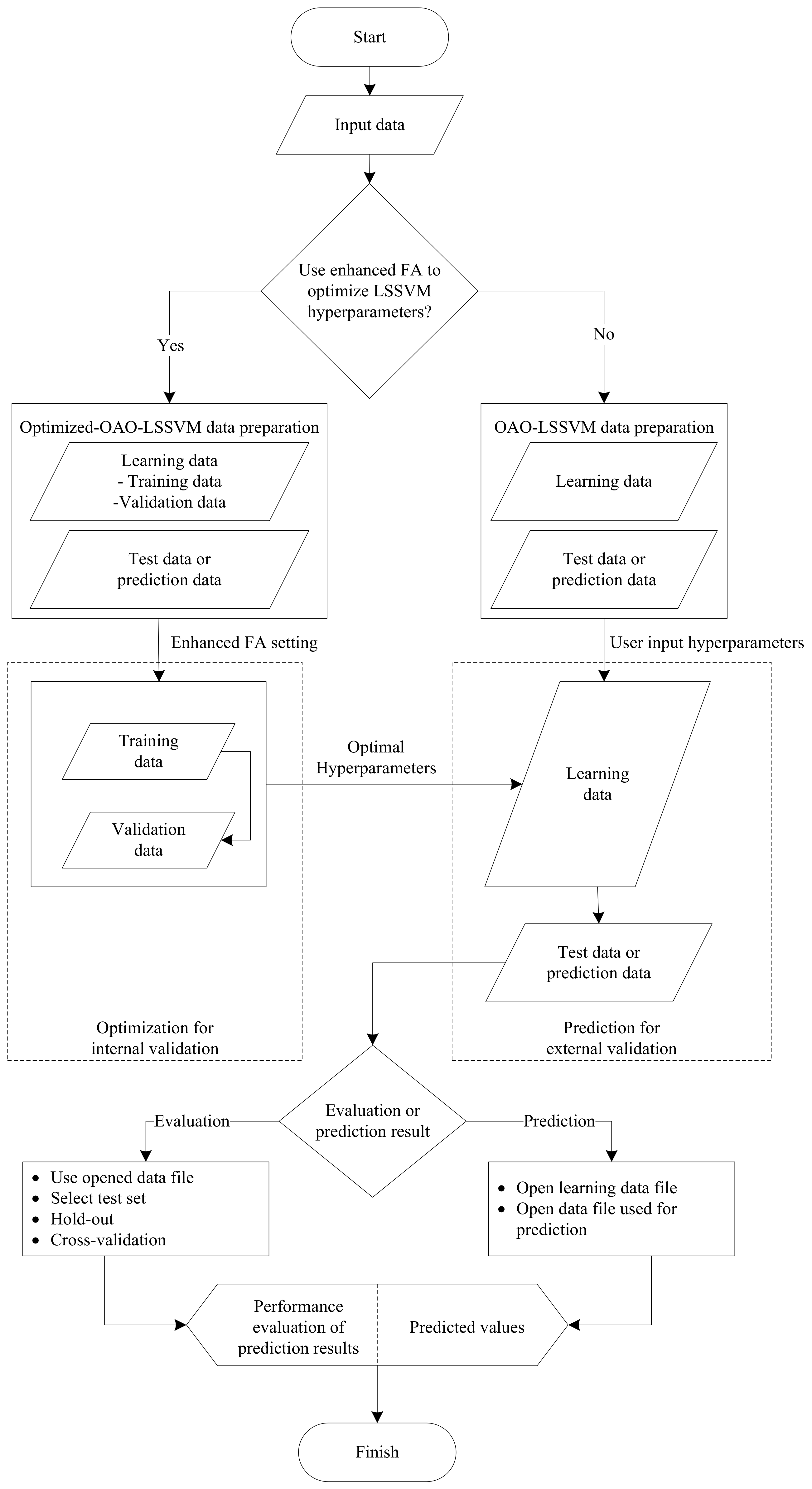
The multi-level classification system comprises two computing modules, OAO-LSSVM and Optimized-OAO-LSSVM. Combining the OAO scheme with the LSSVM yielded the baseline model for solving multi-class classification problems. The LSSVM model was then further optimized using a swarm intelligence algorithm (enhanced FA). The GUI was created to help users to be acquainted with the environment of machine learning.

4.2.1. Framework

Figure 1 shows the framework of the proposed multi-level classification system. The two modules of the system are the Optimized-OAO-LSSVM and baseline OAO-LSSVM module. In the system, the users can choose either the Optimized-OAO-LSSVM or baseline OAO-LSSVM module to run the data. Both modules help the user to evaluate model performance or to predict outputs. The system also enables the user to save the model after executing the training process, allowing it to be reused for other purposes.

With the baseline OAO-LSSVM module, the input data are separated into learning data and test data. After setting original input hyperparameters, the learning data help to create the model, and the test data are used to evaluate model or predict output values depending on the demand of users. The main difference between the Optimized-OAO-LSSVM and baseline module is that the input hyperparameters of the Optimized-OAO-LSSVM model are finetuned by the enhanced FA, which improves the performance of the machine learning model.

4.2.2. Implementation

The proposed system has two functions, including evaluation and prediction. The evaluation function supports four operations, and users can choose one of these four operations.

Figure 2 shows the screenshots of the system. In the main menu, a user can adopt the enhanced FA to tune the LSSVM hyperparameters. Then, the parameters are set by the user, or the default values are used. Next, the user must select or not select normalization, the part between the training data and the validation data, as well as the stopping criteria.

The results and predicted values obtained by using the Optimized-OAO-LSSVM model are displayed in the interface. Moreover, users can view and save the results as an Excel file, which includes inputs and outputs. The Optimized-OAO-LSSVM system showed the efficiency of operating the proposed model.

5. Engineering Applications

This section elucidates the Optimized-OAO-LSSVM system to handle classification issues. Many case studies in engineering management were used herein to evaluate the application of multi-classification system. Section 5.1 presents the results obtained by using the proposed model to solve binary-class geotechnical problems. Section 5.2 demonstrates the use of the system to solve multi-class civil engineering and construction management problems.

5.1. Binary-Class Problems

Two binary-class datasets associated with seismic hazards in coal mines and the early warning of liquefaction disasters are taken from the literature [76,77].

Table 4. Data collection and parameter setting.

Parameter	Unit	Max. Value	Min. Value	Mean	Standard Deviation
Dataset 1—Seismic bumps, 2584 samples, Poland [76]
Genergy	N/A	2,595,650.00	100.00	90,242.52	229,200.51
Gpuls	N/A	4518.00	2.00	538.58	562.65
Gdenergy	N/A	1245.00	−96.00	12.38	80.32
Gdpuls	N/A	838.00	−96.00	4.51	63.17
Energy	Joule	402,000.00	0.00	4975.27	20,450.83
Maxenergy	Joule	400,000.00	0.00	4278.85	19,357.45
Seismic bumps (1 = hazardous state, 2 = not)	N/A	2	1
Dataset 2—Soil Liquefaction, 226 samples, U.S.A., China and Taiwan [77]
Cone tip resistance (qc)	MPa	25.00	0.90	5.82	4.09
Sleeve friction ratio (Rf)	%	5.20	0.10	1.22	1.05
Effective stress (σ’v)	kPa	215.20	22.50	74.65	34.40
Total stress (σv)	kPa	274.00	26.60	106.89	55.36
Horizontal ground surface acceleration (amax)	gal	0.80	0.08	0.29	0.14
Earthquake movement magnitude (Mw)	N/A	7.60	6.00	6.95	0.44
Soil liquefaction (1 = exists, 2 = not)	N/A	2	1

Note: The users have to convert the output of data into class 1 and 2.

presents the variables and their descriptive statistics of the datasets.

In monitoring seismic hazards in coal mines, an early warning model can be applied to forecast the occurrence of hazard events and withdraw workers from threatened areas, reducing the risk of mechanical seismic impact to save the lives of mine workers. The dataset has 170 samples, representing a hazardous state (Class 1) and 2414 samples, representing a non-hazardous state (Class 2).

Soil liquefaction is a major effect of an earthquake and may seriously damage buildings and infrastructure and cause loss of life. The deformation of soil by a high pore-water pressure causes the liquefaction. A soil deposit under a dynamic load generates pore water, which reduces its strength and causes liquefaction. The proposed model is used to predict the liquefaction or non-liquefaction of soil. This database embraces 226 examples comprising 133 instances of liquefaction (Class 1) and 93 instances of non-liquefaction (Class 2).

Chou et al., (2016) combined the smart firefly algorithm with the LSSVM (SFA-LSSVM) to solve seismic bump and soil liquefaction problems [78]. They compared the performance of the SFA-LSSVM model with the experimental performance of other models and concluded that the SFA-LSSM is the best model for solving such problems.

Therefore, to demonstrate the effectiveness and efficiency of the proposed model in solving binary-class problems, the results obtained using the proposed model were compared with those obtained using the SFA-LSSVM model.

Table 5. Comparison of performances of SFA-LSSVM and Optimized-OAO-LSSVM models used to solve binary problems.

Technique	Cross-Fold Validation	Accuracy (%)	Training and Test Time (s)
Dataset 1—Seismic bumps (2584 samples)
SFA-LSSVM (original value)	10	93.46	355,913.59
SFA-LSSVM (feature scaling)	10	93.96	174,328.48
Optimized-OAO-LSSVM (original value)	10	93.42	1136.60
Optimized-OAO-LSSVM (feature scaling)	10	93.30	717.37
Dataset 2—Soil liquefaction (226 samples)
SFA-LSSVM (original value)	10	94.31	19,884.82
SFA-LSSVM (feature scaling)	10	95.18	998.45
Optimized-OAO-LSSVM (original value)	10	93.38	57.22
Optimized-OAO-LSSVM (feature scaling)	10	92.93	56.14

presents the results of using the Optimized-OAO-LSSVM and SFA-LSSVM models for predicting seismic bumps and soil liquefaction in original-value and feature-scaling cases.

The computational time of the Optimized-OAO-LSSVM model was substantially shorter than that of the SFA-LSSVM model, although its predictive accuracy was not significantly higher. With seismic bumps dataset, the Optimized-OAO-LSSVM model had an accuracy of 93.42% in 1136.60 s whereas the SFA-LSSVM model had an accuracy of 93.46% in 355,913.59 s.

Similarly, the Optimized-OAO-LSSVM model had a shorter computing time than the SFA-LSSVM model with soil liquefaction data (57.22 s and 19,884.82 s with original value case, respectively). Therefore, the Optimized-OAO-LSSVM is an effective and efficient model for solving binary-class classification problems.

5.2. Multi-Level Problems

The proposed system was applied to three multi-level cases. The results obtained were compared with those obtained using the baseline model (OAO-LSSVM), with prior experimental results and with those obtained using single multi-class models (SMO, Multiclass Classifier, Naïve Bayes, Logistic, and LibSVM).

5.2.1. Case 1—Diagnosis of Faults in Steel Plates

Fault diagnosis is important in industrial production. For instance, producing defective products can impose a high cost on a manufacturer of steel products. Therefore, in this investigation a dataset of faults in steel plates, which are important raw materials in hundreds of industrial products, is used as a practical case. The original dataset was obtained from Semeion, Research of Sciences of Communication, Via Sersale 117, 00128, Rome, Italy. In this dataset, faults in steel plates are classified into 7 types, including Pastry, Zscratch, Kscratch, Stains, Dirtiness, Bumps and Other. The database contains 1941 data points with 27 independent variables.

To prevent confusion in multi-class classification, Tian et al. [65] eliminated faults of class 7 because that class did not refer to a particular kind of fault. Furthermore, to improve predictive accuracy, they used the recursive feature elimination (RFE) algorithm to reduce the number of dimensions of the multi-classification. Therefore, Tian et al. used a modified steel plates fault dataset (1268 samples) with 20 independent attributes and six types of fault [65]. To obtain a fair comparison, therefore, the proposed model was applied to the modified data.

Table 6. Statistical input and profile of categorical labels for the steel plate faults diagnosis data.

Parameter	Max. Value	Min. Value	Mean	Standard Deviation
Input
Edges Y Index	1	0.048	0.813	0.234
Outside Global Index	1	0	0.576	0.482
Orientation Index	1	−0.991	0.083	0.501
Edges X Index	1	0.014	0.611	0.243
Type of Steel_A300	1	0	0.400	0.490
Luminosity Index	1	−0.999	−0.131	0.149
Square Index	1	0.008	0.571	0.271
Type of Steel_A400	1	0	0.600	0.490
Length of Conveyer	1794	1227	1459.160	144.578
Minimum of Luminosity	203	0	84.549	32.134
X Maximum	1713	4	617.964	497.627
X Minimum	1705	0	571.136	520.691
Sigmoid of Areas	1	0.119	0.585	0.339
Edges Index	1	0	0.332	0.300
Empty Index	1	0	0.414	0.137
Maximum of Luminosity	253	37	130.194	18.691
Log of Areas	51,837	0.301	22,757.224	9704.564
Log Y Index	42,587	0	11,636.590	7273.127
Log X Index	30,741	0.301	9477.470	7727.986
Steel Plate Thickness	300	40	78.738	55.086
Output—Type of fault	N/A
Pastry (Class 1)
ZScratch (Class 2)
KScratch (Class 3)
Stains (Class 4)
Dirtiness (Class 5)
Bumps (Class 6)

presents the inputs and profile of categorical labels for data concerning faults in steel plates.

Accuracy, precision, sensitivity, specificity and AUC are indices used to evaluate the effectiveness of the proposed model. High values indicate favorable performance and vice versa. Accuracy is the most commonly used index.

Table 7. Results of performance measures and rates of improved accuracy achieved by Optimized-OAO-LSSVM.

	Empirical Models Reported in Primary Works and Single Multi-Class Models	Performance Measure					Improved Accuracy by Optimized-OAO-LSSVM System (%)
Dataset		Accuracy (%)	Precision (%)	Sensitivity (%)	Specificity (%)	AUC
Dataset 1—Diagnosis of faults in steel plates	SMO	86.357	86.400	86.300	95.300	0.908	5.191
	Multiclass Classifier	85.726	85.700	85.600	96.000	0.908	5.884
	Naïve Bayes	82.334	82.300	84.440	95.960	0.902	9.608
	Logistic	86.124	86.100	86.000	97.400	0.917	5.447
	LibSVM	31.704	31.700	10.100	89.900	0.500	65.193
	GS-SVM [65]	77.800	-	-	-	-	14.586
	GA-SVM [65]	78.000	-	-	-	-	14.366
	PSO-SVM [65]	79.600	-	-	-	-	12.610
	OAO-LSSVM	53.553	28.764	-	59.148	-	41.206
	Optimized-OAO-LSSVM	91.085	89.995	90.437	91.020	0.907	-
Dataset 2—Quality of water in reservoir	SMO	75.238	75.200	77.500	85.900	0.817	19.661
	Multiclass Classifier	85.397	85.400	86.500	94.900	0.907	8.813
	Naïve Bayes	76.000	76.000	78.700	99.500	0.891	18.847
	Logistic	89.580	89.600	89.600	95.000	0.923	4.346
	LibSVM	80.950	81.000	81.000	87.600	0.843	13.561
	OAO-LSSVM	92.196	90.794	90.633	92.078	0.914	1.553
	Optimized-OAO-LSSVM	93.650	92.531	93.840	93.746	0.938	-
Dataset 3—Urban land cover	SMO	85.778	85.800	86.000	89.000	0.875	1.714
	Multiclass Classifier	64.900	64.900	64.800	99.400	0.821	25.636
	Naïve Bayes	81.000	81.000	81.600	91.800	0.867	7.189
	Logistic	65.926	65.900	65.900	95.300	0.806	24.461
	LibSVM	18.370	18.400	19.000	81.400	0.502	78.951
	k-NN classifier [79]	80.140	-	-	-	-	8.174
	ELM classifier [79]	84.700	-	-	-	-	2.949
	SVM classifier [79]	84.890	-	-	-	-	2.732
	OAO-LSSVM	18.378	11.637	-	-	-	78.942
	Optimized-OAO-LSSVM	87.274	87.048	89.918	87.297	0.886	-

presents the predictive performances of SMO, the Multiclass Classifier, the Naïve Bayes, Logistic, LibSVM and several empirical models [65], and the OAO-LSSVM and Optimized-OAO-LSSVM models when applied to the steel fault dataset.

Tian et al. used three optimizing algorithms—grid search (GS), GA and PSO—combined with SVM to improve the accuracy of classification in the steel fault dataset [65]. They showed that the SVM model, optimized by PSO, was the best for predicting the test data, with an accuracy of 79.6%. With the same data, the Optimized-OAO-LSSVM had an accuracy of 91.085%. The Optimized-OAO-LSSVM model was more accurate than SMO (86.357%), the Multiclass Classifier (85.726%), the Naïve Bayes (82.334%), the Logistic model (86.124%), the LibSVM (31.704%) and the OAO-LSSVM model (53.553%). The statistical accuracy of the Optimized-OAO-LSSVM model, applied to the test data, was better than those of other algorithms at a significance level of 1%.

5.2.2. Case 2—Quality of Water in Reservoir

The case study from the field of hydroelectric engineering involves a dataset on the quality of water in a reservoir. The quality of water is critical because water is a primary natural resource that supports the survival and health of humans through drinking, irrigation, hydroelectricity, aquaculture and recreation. Accurately predicting water quality is essential in the management of water resources.

Table 8. Statistical attributes of reservoir water quality dataset.

Parameter	Max. Value	Min. Value	Mean	Standard Deviation
Input
Secchi disk depth (SD)	8.375	0.1	1.8605	1.1026
Chlorophyll a (Chla)	151.4	0.1	7.9216	12.2305
Total phosphorus (TP)	2.0495	0.0022	0.0677	0.214
Output-Reservoir water quality	N/A
Excellent—Class 1
Good—Class 2
Average—Class 3
Fair—Class 4
Poor—Class 5

shows the details of the water quality dataset. Carlson’s Trophic State Index (CTSI) has long been used in Taiwan to assess eutrophication in reservoirs [80]. Generally, the factors that are considered to evaluate reservoir water quality are quite complex. The key assessment factors include Secchi disk depth (SD), chlorophyll a (Chla), total phosphorus (TP), dissolved oxygen (DO), ammonia (NH3), biochemical oxygen demand (BOD), temperature (TEMP) and others. In this investigation, SD, Chla and TP were used to classify the quality of water in a reservoir. The OECD’s single indicator water quality differentiations (

Table 9. Single indicator water quality differentiations.

Factor/Index	Excellent 1	Good 2	Average 3	Fair 4	Poor 5
Secchi disk depth (SD)	>4.5	4.5–3.7	3.7–2.3	2.3–1.7	<1.7
Chlorophyll a (Chla)	<2	2.0–3.0	3.0–7.0	7.0–10.0	>10
Total phosphorus (TP)	<8	8–12	12–28	28–40	>40
Carlon’s Trophic State Index (CTSI)	<20	20–40	40–50	50–70	>70

) [81] was used to generate the following five levels for each evaluation factor, as follows; excellent (Class 1), good (Class 2), average (Class 3), fair (Class 4) and poor (Class 5). The database includes 1576 data points with three independent inputs (SD, Chla and TP) and the output is one of five ratings of quality of water in a reservoir.

Table 7 compares the performances of the SMO, Multiclass Classifier, Naïve Bayes, Logistic, LibSVM, OAO-LSSVM and Optimized-OAO-LSSVM models when used to predict the quality of water in a reservoir, using test data. The numerical results revealed that the Optimized-OAO-LSSVM is the best model for predicting this dataset in terms of accuracy, precision, sensitivity, specificity and AUC value (93.650% 92.531%, 93.840%, 93.746% and 0.938 respectively). Moreover, the hypothesis tests concerning accuracy established that the Optimized-OAO-LSSVM model was more efficient than the other models at a significance level of 1%.

5.2.3. Case 3—Urban Land Cover

Another dataset, concerning urban land cover (675 data points), was obtained from the UCI Machine Learning Repository [82]. Information about land use is important in every city because it is used for many purposes [83], including tax assessment, setting land use policy, city planning, zoning regulation, analysis of environmental processes, and management of natural resources. The assessment of land cover is very important for scientists and authorities that are concerned with mapping the patterns of land cover on global, regional as well as local scales, to understand geographical changes [79]. Therefore, accurate and readily produced land cover classification maps are of great importance in studies of global change.

The land cover dataset includes a total of 147 features, which include the spectral, magnitude, formal and textural properties of an image of land. The spectral, magnitude, formal and textural properties of the image consist of 21 features. Afterwards, these features were repeated on each coarse scales (20, 40, 60, 80, 100, 120, and 140), yielding 147 features [79].

Table 10. Attribute information in the urban land cover dataset.

Names of Attributes in the Dataset	Source of Information of the Segments
BrdIndx: border index	Shape
Area: area in m2	Size
Round: roundness	Shape
Bright: brightness	Spectral
Compact: compactness	Shape
ShpIndx: shape index	Shape
Mean_G: green	Spectral
Mean_R: red	Spectral
Mean_NIR: near Infrared	Spectral
SD_G: standard deviation of green	Texture
SD_R: standard deviation of red	Texture
SD_NIR: standard deviation of near infrared	Texture
LW: length/width	Shape
GLCM1: gray-level co-occurrence matrix	Texture
Rect: rectangularity	Shape
GLCM2: another gray-level co-occurrence matrix attribute	Texture
Dens: density	Shape
Assym: asymmetry	Shape
NDVI: normalized difference vegetation index	Spectral
BordLngth: border length	Shape
GLCM3: another gray-level co-occurrence matrix attribute	Texture

Note: These attributes are repeated for each coarse scale (i.e., variable_20, variable_40…, variable_140).

shows the features used in the dataset. The data specify nine forms of land cover—trees (Class 1), concrete (Class 2), shadows (Class 3), asphalt (Class 4), buildings (Class 5), grass (Class 6), pools (Class 7), cars (Class 8) and soil (Class 9)—which are treated as the predictive classes, and listed in

Table 11. Number of data points concerning nine forms of land cover in urban land cover dataset.

Names of the Land Cover in the Dataset	No. of Data Points
Trees (Class 1)	106
Concrete (Class 2)	122
Shadow (Class 3)	61
Asphalt (Class 4)	59
Buildings (Class 5)	112
Grass (Class 6)	116
Pools (Class 7)	29
Cars (Class 8)	36
Soil (Class 9)	34
Total	675

.

Durduran [79] used three classification algorithms, k-NN, SVM and extreme learning machine (ELM), each combined with the OAR scheme, to predict urban land cover. To verify the effectiveness of the proposed Optimized-OAO-LSSVM model in classifying urban land cover, the performance of the proposed model is compared with their experimental results.

Table 7 compares the predictive accuracies of the SMO, Multiclass Classifier, Naïve Bayes, Logistic, LibSVM, OAO-LSSVM, and the proposed models with that, experimentally determined, of k-NN, SVM, and ELM. As shown in Table 10, the Optimized-OAO-LSSVM had an accuracy of 87.274%, a precision of 87.048%, a sensitivity of 89.918%, a specificity of 87.297% and an AUC of 0.886. Clearly, the Optimized-OAO-LSSVM model outperformed the other models in all these respects. Notably, the Optimized-OAO-LSSVM model is more efficient than the other models at a significance level of 1%.

5.3. Analytical Results and Discussion

The performance of the proposed classification system was evaluated in terms of accuracy, precision, sensitivity, specificity and AUC. High values of these indices revealed favorable performance and vice versa. However, accuracy is the most commonly used for comparison. Table 7 summarizes the values of the performance metrics in case studies 1–3. The applicability and efficiency of the proposed system were confirmed by comparing its performance with other single multi-class and previous models.

Data preprocessing, such as data cleansing and transformation, is essential to improving the results of data analysis [84]. The user can decide whether or not to normalize data to the (0, 1) range. Normalizing a dataset can minimize the effect of scaling.

Table 12. Analytical results obtained using Optimized-OAO-LSSVM.

Dataset		Performance Measure
		Accuracy (%)	Precision (%)	Sensitivity (%)	Specificity (%)	AUC
Dataset 1—Diagnosis of faults in steel plates
	Original value	91.085	89.995	90.437	91.020	0.907
	Feature scaling	88.646	86.518	88.458	88.620	0.885
Dataset 2—Quality of water in reservoir
	Original value	93.526	92.335	94.272	93.622	0.939
	Feature scaling	93.650	92.531	93.840	93.746	0.938
Dataset 3—Urban land cover
	Original value	87.274	87.048	89.918	87.297	0.886
	Feature scaling	86.521	86.003	87.310	86.534	0.874

presents the results of applying the proposed system in the three case studies with the original data and the data after feature scaling. In Table 12, better predictive accuracies were obtained with the original steel plates fault and land cover datasets (91.085% and 87.274%, respectively), whereas better results were obtained with the reservoir water quality dataset after feature scaling (93.650%).

6. Conclusions and Recommendation

This work proposed a hybrid inference model that integrated an enhanced firefly algorithm (enhanced FA) with a least squares support vector machine (LSSVM) model and decomposition strategy (i.e., one-against-one, OAO) to improve its predictive accuracy in solving multi-level classification problems. The proposed system provides a baseline classification model, called OAO-LSSVM. The effectiveness of the enhanced FA Optimized-OAO-LSSVM model is compared with that of the baseline OAO-LSSVM model.

To verify the applicability and efficiency of the proposed model in solving multi-level classification problems, the predictive performance of the model was compared to other multi-classification methods and prior studies with respect to accuracy, precision, sensitivity, specificity and AUC. Three case studies, involving the multi-class problems of categorizing steel plate faults, assessing the water quality in a reservoir, and managing the condition of urban land cover, were considered. The proposed model exhibited higher predictive accuracy than the baseline model (OAO-LSSVM), experimental studies and other single multi-class algorithms with the highest accuracy in each case. In particular, the proposed model yielded 91.085%, 93.650% and 87.274% accuracy in steel plate faults, water quality in a reservoir, and urban land cover, respectively. Therefore, the model can be used as a decision-making tool in solving practical problems in the fields of civil engineering and construction management.

A main contribution of this work is the extension of a binary-class model to a meta-heuristically optimized multi-level model for efficiently and effectively solving classification problems involving multi-class data. Another major contribution is the design of an intelligent computing system for users with ease that was proved to be an effective project management software. Although the proposed model exhibited excellent predictive accuracy, and a graphical user interface was effectively implemented, it has limitations that should be addressed by future studies. The proposed model does not have high predictive accuracy when applied to small datasets or the unbalanced numbers of data points. Future studies should also improve the model to make it useful for solving multiple inputs and multiple outputs of multiclass classification problems, and develop it in a cloud computing environment to increase its ubiquitous applicability.

References

1. Sesmero, M.P.; Alonso-Weber, J.M.; Gutierrez, G.; Ledezma, A.; Sanchis, A. An ensemble approach of dual base learners for multi-class classification problems. Inf. Fusion 2015, 24, 122–136. [Google Scholar] [CrossRef]
2. Khaledian, Y.; Miller, B.A. Selecting appropriate machine learning methods for digital soil mapping. Appl. Math. Model. 2020, 81, 401–418. [Google Scholar] [CrossRef]
3. Wang, Q.; Li, Q.; Wu, D.; Yu, Y.; Tin-Loi, F.; Ma, J.; Gao, W. Machine learning aided static structural reliability analysis for functionally graded frame structures. Appl. Math. Model. 2020, 78, 792–815. [Google Scholar] [CrossRef]
4. Bhardwaj, A.; Tiwari, A. Breast cancer diagnosis using Genetically Optimized Neural Network model. Expert Syst. Appl. 2015, 42, 4611–4620. [Google Scholar] [CrossRef]
5. Iounousse, J.; Er-Raki, S.; El Motassadeq, A.; Chehouani, H. Using an unsupervised approach of Probabilistic Neural Network (PNN) for land use classification from multitemporal satellite images. Appl. Soft Comput. 2015, 30, 1–13. [Google Scholar] [CrossRef]
6. Huang, N.; Xu, D.; Liu, X.; Lin, L. Power quality disturbances classification based on S-transform and probabilistic neural network. Neurocomputing 2012, 98, 12–23. [Google Scholar] [CrossRef]
7. Del Vecchio, C.; Fenu, G.; Pellegrino, F.A.; Di Foggia, M.; Quatrale, M.; Benincasa, L.; Iannuzzi, S.; Acernese, A.; Correra, P.; Glielmo, L. Support Vector Representation Machine for superalloy investment casting optimization. Appl. Math. Model. 2019, 72, 324–336. [Google Scholar] [CrossRef]
8. Kaefer, F.; Heilman, C.M.; Ramenofsky, S.D. A neural network application to consumer classification to improve the timing of direct marketing activities. Comput. Oper. Res. 2005, 32, 2595–2615. [Google Scholar] [CrossRef]
9. Karakatič, S.; Podgorelec, V. Improved classification with allocation method and multiple classifiers. Inf. Fusion 2016, 31, 26–42. [Google Scholar] [CrossRef]
10. Wang, Z.Z.; Zhang, Z. Seismic damage classification and risk assessment of mountain tunnels with a validation for the 2008 Wenchuan earthquake. Soil Dyn. Earthq. Eng. 2013, 45, 45–55. [Google Scholar] [CrossRef]
11. Chou, J.-S.; Hsu, S.-C.; Lin, C.-W.; Chang, Y.-C. Classifying Influential Information to Discover Rule Sets for Project Disputes and Possible Resolutions. Int. J. Proj. Manag. 2016, 34, 1706–1716. [Google Scholar] [CrossRef]
12. Hsu, C.-W.; Lin, C.-J. A comparison of methods for multiclass support vector machines. IEEE Trans. Neural Netw. 2002, 13, 415–425. [Google Scholar] [CrossRef] [PubMed] [Green Version]
13. Lorena, A.C.; de Carvalho, A.C.P.L.F.; Gama, J.M.P. A review on the combination of binary classifiers in multiclass problems. Artif. Intell. Rev. 2009, 30, 19. [Google Scholar] [CrossRef]
14. Pal, M. Multiclass Approaches for Support Vector Machine Based Land Cover Classification. arXiv 2008, arXiv:0802.2411, 1–16. [Google Scholar]
15. Rifkin, R.; Klautau, A. In Defense of One-Vs-All Classification. J. Mach. Learn. Res. 2004, 5, 101–141. [Google Scholar]
16. Galar, M.; Fernández, A.; Barrenechea, E.; Bustince, H.; Herrera, F. An overview of ensemble methods for binary classifiers in multi-class problems: Experimental study on one-vs-one and one-vs-all schemes. Pattern Recognit. 2011, 44, 1761–1776. [Google Scholar] [CrossRef]
17. Perner, P.; Vingerhoeds, R. Special issue data mining and machine learning. Eng. Appl. Artif. Intell. 2009, 22, 1–2. [Google Scholar] [CrossRef]
18. Vapnik, V.N. Statistical Learning Theory; John Wiley and Sons: New York, NY, USA, 1998. [Google Scholar]
19. Hall, M.; Frank, E.; Holmes, G.; Pfahringer, B.; Reutemann, P.; Witten, I.H. The WEKA data mining software: An update. SIGKDD Explor. Newsl. 2009, 11, 10–18. [Google Scholar] [CrossRef]
20. Galar, M.; Fernández, A.; Barrenechea, E.; Herrera, F. DRCW-OVO: Distance-based relative competence weighting combination for One-vs-One strategy in multi-class problems. Pattern Recognit. 2015, 48, 28–42. [Google Scholar] [CrossRef]
21. Kang, S.; Cho, S.; Kang, P. Constructing a multi-class classifier using one-against-one approach with different binary classifiers. Neurocomputing 2015, 149, 677–682. [Google Scholar] [CrossRef]
22. Balazs, J.A.; Velásquez, J.D. Opinion Mining and Information Fusion: A survey. Inf. Fusion 2016, 27, 95–110. [Google Scholar] [CrossRef]
23. Medhat, W.; Hassan, A.; Korashy, H. Sentiment analysis algorithms and applications: A survey. Ain Shams Eng. J. 2014, 5, 1093–1113. [Google Scholar] [CrossRef] [Green Version]
24. Yang, X.; Yu, Q.; He, L.; Guo, T. The one-against-all partition based binary tree support vector machine algorithms for multi-class classification. Neurocomputing 2013, 113, 1–7. [Google Scholar] [CrossRef]
25. Kim, K.-j.; Ahn, H. A corporate credit rating model using multi-class support vector machines with an ordinal pairwise partitioning approach. Comput. Oper. Res. 2012, 39, 1800–1811. [Google Scholar] [CrossRef]
26. Chou, J.-S.; Pham, A.-D. Nature-inspired metaheuristic optimization in least squares support vector regression for obtaining bridge scour information. Inf. Sci. 2017, 399, 64–80. [Google Scholar] [CrossRef]
27. Van Gestel, T.; Suykens, J.A.K.; Baesens, B.; Viaene, S.; Vanthienen, J.; Dedene, G.; de Moor, B.; Vandewalle, J. Benchmarking Least Squares Support Vector Machine Classifiers. Mach. Learn. 2004, 54, 5–32. [Google Scholar] [CrossRef]
28. Parouha, R.P.; Das, K.N. An efficient hybrid technique for numerical optimization and applications. Comput. Ind. Eng. 2015, 83, 193–216. [Google Scholar] [CrossRef]
29. Hanafi, R.; Kozan, E. A hybrid constructive heuristic and simulated annealing for railway crew scheduling. Comput. Ind. Eng. 2014, 70, 11–19. [Google Scholar] [CrossRef] [Green Version]
30. Setak, M.; Feizizadeh, F.; Tikani, H.; Ardakani, E.S. A bi-level stochastic optimization model for reliable supply chain in competitive environments: Hybridizing exact method and genetic algorithm. Appl. Math. Model. 2019, 75, 310–332. [Google Scholar] [CrossRef]
31. Dabiri, N.; Tarokh, M.J.; Alinaghian, M. New mathematical model for the bi-objective inventory routing problem with a step cost function: A multi-objective particle swarm optimization solution approach. Appl. Math. Model. 2017, 49, 302–318. [Google Scholar] [CrossRef]
32. Janardhanan, M.N.; Li, Z.; Bocewicz, G.; Banaszak, Z.; Nielsen, P. Metaheuristic algorithms for balancing robotic assembly lines with sequence-dependent robot setup times. Appl. Math. Model. 2019, 65, 256–270. [Google Scholar] [CrossRef] [Green Version]
33. Zhang, J.; Xiao, M.; Gao, L.; Pan, Q. Queuing search algorithm: A novel metaheuristic algorithm for solving engineering optimization problems. Appl. Math. Model. 2018, 63, 464–490. [Google Scholar] [CrossRef]
34. Qingjie, L.; Guiming, C.; Xiaofang, L.; Qing, Y. Genetic algorithm based SVM parameter composition optimization. Comput. Appl. Softw. 2012, 4, 29. [Google Scholar]
35. Rastegar, S.; Araújo, R.; Mendes, J. Online identification of Takagi–Sugeno fuzzy models based on self-adaptive hierarchical particle swarm optimization algorithm. Appl. Math. Model. 2017, 45, 606–620. [Google Scholar] [CrossRef]
36. Pal, S.K.; Rai, C.S.; Singh, A.P. Comparative study of firefly algorithm and particle swarm optimization for noisy non-linear optimization problems. Int. J. Intell. Syst. Appl. 2012, 4, 50–57. [Google Scholar] [CrossRef]
37. Olamaei, J.; Moradi, M.; Kaboodi, T. A new adaptive modified Firefly Algorithm to solve optimal capacitor placement problem. In Proceedings of the 18th Electric Power Distribution Conference, Kermanshah, Iran, 30 April–1 May 2013; pp. 1–6. [Google Scholar]
38. Chou, J.-S.; Pham, A.-D. Enhanced artificial intelligence for ensemble approach to predicting high performance concrete compressive strength. Constr. Build. Mater. 2013, 49, 554–563. [Google Scholar] [CrossRef]
39. Coelho, L.d.S.; Mariani, V.C. Improved firefly algorithm approach applied to chiller loading for energy conservation. Energy Build. 2013, 59, 273–278. [Google Scholar] [CrossRef]
40. Chou, J.-S.; Lin, C. Predicting Disputes in Public-Private Partnership Projects: Classification and Ensemble Models. J. Comput. Civ. Eng. 2013, 27, 51–60. [Google Scholar] [CrossRef]
41. Cheng, M.-Y.; Hoang, N.-D. Risk Score Inference for Bridge Maintenance Project Using Evolutionary Fuzzy Least Squares Support Vector Machine. J. Comput. Civ. Eng. 2014, 28, 04014003. [Google Scholar] [CrossRef]
42. Pant, P.; Chatterjee, D. Prediction of clad characteristics using ANN and combined PSO-ANN algorithms in laser metal deposition process. Surf. Interfaces 2020, 21, 100699. [Google Scholar] [CrossRef]
43. Noori, N.; Kalin, L.; Isik, S. Water quality prediction using SWAT-ANN coupled approach. J. Hydrol. 2020, 590, 125220. [Google Scholar] [CrossRef]
44. Sujith, M.; Jeon, J.-S. Machine Learning–Based Failure Mode Recognition of Circular Reinforced Concrete Bridge Columns: Comparative Study. J. Struct. Eng. 2019, 145, 04019104. [Google Scholar]
45. Vapnik, V.N. The Nature of Statistical Learning Theory; Springer: Berlin/Heidelberg, Germany, 1995. [Google Scholar]
46. Liu, Y.; Wang, H.; Zhang, H.; Liber, K. A comprehensive support vector machine-based classification model for soil quality assessment. Soil Tillage Res. 2016, 155, 19–26. [Google Scholar] [CrossRef]
47. Gholami, R.; Rasouli, V.; Alimoradi, A. Improved RMR Rock Mass Classification Using Artificial Intelligence Algorithms. Rock Mech. Rock Eng. 2013, 46, 1199–1209. [Google Scholar] [CrossRef]
48. Liao, Y.; Xu, J.; Wang, W. A Method of Water Quality Assessment Based on Biomonitoring and Multiclass Support Vector Machine. Procedia Environ. Sci. 2011, 10, 451–457. [Google Scholar] [CrossRef] [Green Version]
49. Du, S.; Liu, C.; Xi, L. A Selective Multiclass Support Vector Machine Ensemble Classifier for Engineering Surface Classification Using High Definition Metrology. J. Manuf. Sci. Eng. 2015, 137, 011003. [Google Scholar] [CrossRef]
50. Polat, K.; Güneş, S. A novel hybrid intelligent method based on C4.5 decision tree classifier and one-against-all approach for multi-class classification problems. Expert Syst. Appl. 2009, 36, 1587–1592. [Google Scholar] [CrossRef]
51. Garcia, L.P.F.; Sáez, J.A.; Luengo, J.; Lorena, A.C.; de Carvalho, A.C.P.L.F.; Herrera, F. Using the One-vs-One decomposition to improve the performance of class noise filters via an aggregation strategy in multi-class classification problems. Knowl. Based Syst. 2015, 90, 153–164. [Google Scholar] [CrossRef]
52. Zhou, L.; Tam, K.P.; Fujita, H. Predicting the listing status of Chinese listed companies with multi-class classification models. Inf. Sci. 2016, 328, 222–236. [Google Scholar] [CrossRef]
53. Suykens, J.A.K.; Gestel, T.V.; Brabanter, J.D.; Moor, B.D.; Vandewalle, J. Least Squares Support Vector Machines; World Scientific: Singapore, 2002. [Google Scholar]
54. Khemchandani, R.; Jayadeva; Chandra, S. Regularized least squares fuzzy support vector regression for financial time series forecasting. Expert Syst. Appl. 2009, 36, 132–138. [Google Scholar] [CrossRef]
55. Haifeng, W.; Dejin, H. Comparison of SVM and LS-SVM for Regression. In Proceedings of the 2005 International Conference on Neural Networks and Brain, Beijing, China, 13–15 October 2005; pp. 279–283. [Google Scholar]
56. Yang, X.-S. Firefly Algorithm; Luniver Press: Bristol, UK, 2008. [Google Scholar]
57. Banati, H.; Bajaj, M. Fire Fly Based Feature Selection Approach. Int. J. Comput. Sci. Issues 2011, 8, 473–479. [Google Scholar]
58. Fister, I.; Fister, I., Jr.; Yang, X.-S.; Brest, J. A comprehensive review of firefly algorithms. Swarm Evol. Comput. 2013, 13, 34–46. [Google Scholar] [CrossRef] [Green Version]
59. Khadwilard, A.; Chansombat, S.; Thepphakorn, T.; Thapatsuwan, P.; Chainate, W.; Pongcharoen, P. Application of Firefly Algorithm and Its Parameter Setting for Job Shop Scheduling. J. Ind. Technol. 2012, 8, 49–58. [Google Scholar]
60. Aungkulanon, P.; Chai-ead, N.; Luangpaiboon, P. Simulated Manufacturing Process Improvement via Particle Swarm Optimisation and Firefly Algorithms. In Lectures Notes Engineering and Computer Science; Newswood Limited: Hong Kong, China, 2011. [Google Scholar]
61. Aci, M.; İnan, C.; Avci, M. A hybrid classification method of k nearest neighbor, Bayesian methods and genetic algorithm. Expert Syst. Appl. 2010, 37, 5061–5067. [Google Scholar] [CrossRef]
62. Chou, J.-S.; Cheng, M.-Y.; Wu, Y.-W. Improving classification accuracy of project dispute resolution using hybrid artificial intelligence and support vector machine models. Expert Syst. Appl. 2013, 40, 2263–2274. [Google Scholar] [CrossRef]
63. Lee, Y.; Lee, J. Binary tree optimization using genetic algorithm for multiclass support vector machine. Expert Syst. Appl. 2015, 42, 3843–3851. [Google Scholar] [CrossRef]
64. Seera, M.; Lim, C.P. A hybrid intelligent system for medical data classification. Expert Syst. Appl. 2014, 41, 2239–2249. [Google Scholar] [CrossRef]
65. Tian, Y.; Fu, M.; Wu, F. Steel plates fault diagnosis on the basis of support vector machines. Neurocomputing 2015, 151, 296–303. [Google Scholar] [CrossRef]
66. García-Pedrajas, N.; Ortiz-Boyer, D. An empirical study of binary classifier fusion methods for multiclass classification. Inf. Fusion 2011, 12, 111–130. [Google Scholar] [CrossRef]
67. Yang, X.-S. Nature-Inspired Metaheuristic Algorithms; Luniver Press: Beckington, UK, 2008; p. 128. [Google Scholar]
68. Hong, W.-C.; Dong, Y.; Chen, L.-Y.; Wei, S.-Y. SVR with hybrid chaotic genetic algorithms for tourism demand forecasting. Appl. Soft Comput. 2011, 11, 1881–1890. [Google Scholar] [CrossRef]
69. Gandomi, A.H.; Yang, X.S.; Talatahari, S.; Alavi, A.H. Firefly algorithm with chaos. Commun. Nonlinear Sci. Numer. Simul. 2013, 18, 89–98. [Google Scholar] [CrossRef]
70. Li, X.; Niu, P.; Liu, J. Combustion optimization of a boiler based on the chaos and Lévy flight vortex search algorithm. Appl. Math. Model. 2018, 58, 3–18. [Google Scholar] [CrossRef]
71. Kohavi, R. A study of cross-validation and bootstrap for accuracy estimation and model selection. In Proceedings of the 14th International Joint Conference on Artificial Intelligence—Volume 2, Montreal, QC, Canada, 20 August 1995; pp. 1137–1143. [Google Scholar]
72. Chou, J.-S.; Tsai, C.-F.; Lu, Y.-H. Project dispute prediction by hybrid machine learning techniques. J. Civ. Eng. Manag. 2013, 19, 505–517. [Google Scholar] [CrossRef]
73. Sokolova, M.; Lapalme, G. A systematic analysis of performance measures for classification tasks. Inf. Process. Manag. 2009, 45, 427–437. [Google Scholar] [CrossRef]
74. Jamil, M.; Yang, X.-S. A Literature Survey of Benchmark Functions For Global Optimization Problems. Int. J. Math. Model. Numer. Optim. 2013, 4, 150–194. [Google Scholar]
75. Surjanovic, S.; Bingham, D. Virtual Library of Simulation Experiments: Test Functions and Datasets. Available online: http://www.sfu.ca/~ssurjano/optimization.html (accessed on 8 May 2016).
76. Sikora, M.; Wróbel, Ł. Application of rule induction algorithms for analysis of data collected by seismic hazard monitoring systems in coal mines. Arch. Min. Sci. 2010, 55, 91–114. [Google Scholar]
77. Goh, A.T.C.; Goh, S.H. Support vector machines: Their use in geotechnical engineering as illustrated using seismic liquefaction data. Comput. Geotech. 2007, 34, 410–421. [Google Scholar] [CrossRef]
78. Chou, J.-S.; Thedja, J.P.P. Metaheuristic optimization within machine learning-based classification system for early warnings related to geotechnical problems. Autom. Constr. 2016, 68, 65–80. [Google Scholar] [CrossRef]
79. Durduran, S.S. Automatic classification of high resolution land cover using a new data weighting procedure: The combination of k-means clustering algorithm and central tendency measures (KMC–CTM). Appl. Soft Comput. 2015, 35, 136–150. [Google Scholar] [CrossRef]
80. Chou, J.-S.; Ho, C.-C.; Hoang, H.-S. Determining quality of water in reservoir using machine learning. Ecol. Inform. 2018, 44, 57–75. [Google Scholar] [CrossRef]
81. Hydrotech Research Institute of National Taiwan University. Reservoir Eutrophiction Prediction and Prevention by Using Remote Sensing Technique. Water Resources Agency: Taipei, Taiwan, 2005. (In Chinese) [Google Scholar]
82. Lichman, M. UCI Machine Learning Repository; University of California, School of Information and Computer Science: Irvine, CA, USA, 2013; Available online: http://archive.ics.uci.edu/ml (accessed on 20 December 2015).
83. Wentz, E.A.; Stefanov, W.L.; Gries, C.; Hope, D. Land use and land cover mapping from diverse data sources for an arid urban environments. Comput. Environ. Urban Syst. 2006, 30, 320–346. [Google Scholar] [CrossRef]
84. Crone, S.; Guajardo, J.; Weber, R. The impact of preprocessing on support vector regression and neural networks in time series prediction. In Proceedings of the International Conference on Data Mining DMIN’06, Las Vegas, NV, USA, 26–29 June 2006; pp. 37–42. [Google Scholar]
Figure 1. Metaheuristic-optimized multi-level classification system flowchart.
Applsci 11 05533 g001
Figure 2. Screenshots of system.
Applsci 11 05533 g002