Development of Parameters towards Voice Bifurcations

Abstract

Pathological vocal folds are known to exhibit multiple oscillation patterns, depending on tissue imbalance, subglottal pressure level, and other factors. This includes mid-phonation changes due to bifurcations in the underlying voice source system. Knowledge of when changes in oscillation patterns occur is helpful in the assessments of voice disorders, and the knowledge could be transformed into useful objective measures. Mid-phonation bifurcations can occur in rapid succession; hence, a fast classification of oscillation pattern is critical to minimize the averaging of data across bifurcations. This paper proposes frequency-ratio based short-term measures, named harmonic disturbance factor (HDF) and biphonic index (BI), towards the detection of the bifurcations. For the evaluation of HDF and BI, a frequency selection algorithm for glottal source signals is devised, and its efficacy is demonstrated with the glottal area waveforms of four cases, representing the wide range of oscillatory behaviors. The HDF and BI exhibit clear transitions when the voice bifurcations are apparent in the spectrograms. The presented proof-of-concept experiment’s outcomes warrant a larger scale study to formalize the parameters of the frequency selection algorithm.

1. Introduction

Normal healthy voice exhibits a nearly periodic behavior, which can be readily observed in its acoustic or glottal source signals via spectral visualization techniques such as spectrogram, power spectrum, or cepstrogram. Voice pathology, however, often introduces interference to the vibration of vocal folds, forcing them to oscillate without collision or out of sync or sometimes even chaotically [1,2]. Such disruptions directly translate to a loss of voice quality, often described as hoarse, rough, breathy, or strained.

The pathological interference of vocal fold oscillation leads to an anomaly in voice signals. To classify voice signals, the Workshop on Acoustic Voice Analysis [3] in 1994 recommended the use of the following voice signal types:

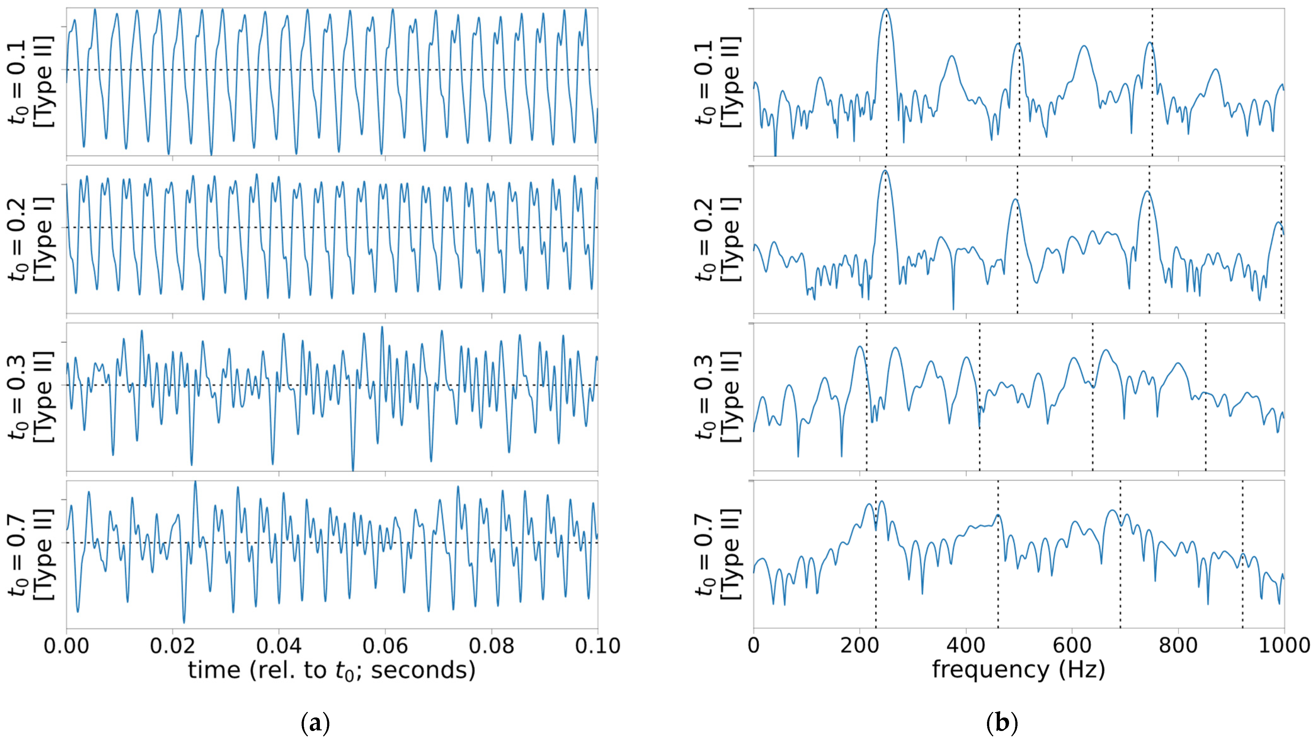
• Type I—nearly periodic;
• Type II—contain intermittency, strong subharmonics, or modulations; and
• Type III—chaotic or random.

These types are used throughout the paper. Classification of these types were suggested to be done via visual inspection of the spectrogram of the voice signal under study. To date, no commercial or publicly accessible software is available to classify the voice types automatically, although there is a long-standing active research effort [4,5,6,7,8] applying concepts from dynamical systems theory. This paper approaches this classification problem based on the Type-II voice characteristics.

Type II encompasses a broad spectrum of voicing patterns. It could be summarized as follows: A voice signal consists of clean tonal components but not all components belong to the harmonic series with an obvious speaking fundamental frequency. These extraneous (or non-harmonic) tonal components, which could appear intermittently during phonation, disturb the audibly pleasant harmonic composition of a healthy voice and contribute to the perceived roughness in the voice [9]. The non-harmonic components include period-$n$ subharmonics and biphonia—the coexistence of two harmonic series with unrelated fundamental frequencies. The pathological Type-II voice may also exhibit intermittency or mid-phonation changes [10,11,12], switching between multiple modes of oscillation, with or without non-harmonic components. The variation in oscillation modes can be explained by the dynamic systems theory [10,13,14,15]. Dynamical systems may have bifurcation points, where a small change in system parameters results in a large change in system behavior. For the voice system, the system parameters include the subglottal pressure and the vocal fold mass and stiffness. Bifurcation diagrams are often used to visualize these bifurcation points.

With an asymmetric vocal fold model of superior nerve paralysis, a two-parameter bifurcation diagram in the asymmetry factor and subglottal pressure (Figure 7 in [13]) suggests a large number of possible oscillation modes (or attractors of a dynamical system) that represent all three voice types. There is one oscillation mode each for Type I and III, and the rest are different Type-II modes with different phase-locking modes (i.e., different subharmonic periods and biphonia frequency ratios) [15]. Asymmetric vocal folds vibration mode can switch suddenly from Type I to Type II or III, or vice versa as the subglottal pressure fluctuates during phonation. The model also suggests that severe asymmetry may lead to multiple Type-II modes during phonation. These observations from the theoretical model are in agreement with the observation of pathological voice, which can exhibit mid-phonation voice change [10,11,12]. It is possible for the bifurcations to occur in a rapid succession, and one such case is included in this paper (Case 3). Some of its oscillation modes in its acoustic signal are captured in Figure 1.

There are objective parameters that explicitly target the spectral features of Type-II voice. In the context of digital telephone systems, subharmonic-to-harmonic ratio [17,18] was introduced to improve the pitch determination performance and was later applied to assess the pathological subharmonics [19]. The Degree of Subharmonics (DSH) parameter in the Multi-Dimensional Voice Program (MDVP) [20] measures the percentage of time the subharmonic is present. Aichinger et al. [21] devised the Diplophonia Diagram, which characterizes the signal under study by the residuals of two modeling outcomes using single harmonic series vs. two harmonic series. Awan and Awan [22] proposed a tandem of cepstrum peak prominence measures to quantify the degree of presence of subharmonics and demonstrated an 82.2% correct classification of rough vs. non-rough voice.

Kramer et al. [23] studied the relationship between cycle-to-cycle variability in the fundamental frequency $F_0$ and percentage of low $F_0$ estimates on connected speech to the perceived roughness. Kramer’s work is unique among others because it focuses on the frequency measure rather than measures based on signal strength or power. This remark from their work is noteworthy: “Because the presence of subharmonics is the main source of both pitch perception and $F_0$ detection errors, it seems reasonable to exploit errors in $F_0$ detection for quantitative measurement of pathologic voices.” For Type-I voice, $F_0$ detection error seldom happens (assuming clean signal) while Type II induces error because of the strong non-harmonic content residing near the first harmonic (relative to the second harmonic frequency). In the case of biphonia, there exist two different $F_{0}s$ that are close in both frequency and power. This leads to the seed idea for this paper: the spectral peak characteristics are vastly different between Type-I and Type-II voices, and analyzing the relative positions of the peaks may result in differentiating Type-I and Type-II signals.

We apply this idea towards detecting mid-phonation bifurcations, especially between Type I and Type II. The voice type detection scheme can also be devised from Type-III signals, namely by deploying the methods based on dynamical systems analysis and chaos theory. There are a number of studies available, exploring different methodologies, e.g., correlation dimensions [4,5,24,25,26], Lyapunov exponent [4,25], diffusive chaos [6], nonlinear energy difference ratio [7], recurrence quantification measures [27,28], and intrinsic dimension [5]. To detect mid-phonation bifurcations, these methods are challenged by their data duration requirements. Typical analysis durations range from 0.2 to 2 s, while the bifurcations could occur at a more frequent rate, as shown in Figure 1.

Main Concept

This paper focuses on the detection of mid-phonation bifurcations in pathological voice. The underlying motivation for such detection scheme is twofold. First, automatic segmentation of voice signal helps the selection of voice analysis methods and objective parameters. For example, the perturbation analysis is limited to Type-I signals [3]. Second, the detection outcomes (e.g., the number of mid-phonation bifurcations) can be used as objective measures, similar to MDVP’s DSH measure but targeting broader Type-II characteristics. Frequent mid-phonation voice change can be perceived as poor voice quality, possibly worse than consistent Type-II or Type-III voice. As such, objective measures of bifurcations are potential strong contributors to objective voice assessment tools.

To be able to detect frequent bifurcations as seen in Figure 1, a signal window length of shorter than 100 ms is desired. Two measures, named harmonic disturbance factor (HDF) and biphonia index (BI), are proposed to be used for this task. The biphonic and subharmonic spectral contents of Type-II voice are shown to have at least comparable strength to the second harmonic of such voice [29]. This observation leads to a family of voice parameters based on the frequencies of the spectral peaks. The basic premise here is to pick two spectral peaks: one, labeled $f_0$, which corresponds to $F_0$ of the voice, and another, labeled $f_1$, which is indicative of the active voice type (Type I vs. Type II/III). The selection strategy of the second peak is critical, and this paper proposes a strategy for glottal source signals. Given these peaks, the ratio of these two frequencies is used to normalize the effect of the fundamental frequency; this ratio is defined as:

$$\mathsf{\gamma } =\frac{f_1}{f_0}.$$

(1)

Table 1. Expectation of Frequency Estimates ¹.

Voice Type	${\mathit{f}}_0$	${\mathit{f}}_1$	$\mathsf{\gamma }$
Type I	$F_0$	$n{F}_0$, $n\in \left\{2,3,\dots \right\}$	$n\ge 2$
Type II—Period-$m$ Subharmonic	$F_0$	$n{F}_0/m$, $n\in \left\{1,2,\dots \right\}\setminus \left\{N\right\}$	$n/m\ncong 1$
Type II—Biphonia	$F_{0,1}$	$F_{0,2}$, near $F_{0,1}$	$~1.0$
Type III	$F_0$ if prevalent otherwise random	Random	Random

¹ $F_0$: fundamental frequency, $F_{0,1}, F_{0,2}$: fundamental frequencies of two competing harmonic series.

summarizes the expected behaviors of the three quantities: $f_0$, $f_1$, and $\mathsf{\gamma }$. There is a clear segmentation in the expected values with three caveats. First, the measures of Type-III voice are expected to be random, and thus the estimates are inconsistent across successive observation windows, unlike the other voice types. Second, $f_1$ for the Type-II voice with subharmonics could align with the proper pitch harmonic frequencies ($n{f}_0$), in which case it cannot be distinguished from Type I. Third, the strengths of the two spectral peaks of biphonic voice could be similar, thus their fundamental frequency, $f_{0,1}$ and $f_{0,2}$, assignments to $f_0$ and $f_1$ may switch back and forth across the phonation. With these caveats in mind, two short-term parameters on the frequency ratio and its expectations for each voice type are proposed as follows.

Harmonic Disturbance Factor (HDF):

A short-term, narrowband voice measure to penalize if $f_1$is not a higher harmonic frequency than $f_0$. Given the frequency ratio $\mathsf{\gamma }$defined in (1), the HDF $\in \left[0.0, 2.0\right]\setminus \left\{1.0\right\}$ is defined by:

$$\mathrm{HDF} =\{\begin{array}{ll}\left|2-\mathsf{\gamma }\right|\hfill & \mathrm{if} \mathsf{\gamma }\le 2,\hfill \\ \left|\mathsf{\gamma } \mathrm{mod} 1\right|\hfill & \mathrm{if} \mathsf{\gamma }>2 \mathrm{and} \left(\mathsf{\gamma } \mathrm{mod} 1\right)\le 0.5,\hfill \\ \left|1-\mathsf{\gamma } \mathrm{mod} 1\right|\hfill & \mathrm{otherwise}\hfill \end{array}$$

(2)

where (a$mod b$) is the modulo operator. The HDF is expected to be zero if the voice is Type I and non-zero for Type-II voice.

Biphonia Index (BI):

A short-term, narrowband voice measure to indicate the likelihood of vocal folds vibrating with two unrelated frequencies. Given the frequency ratio$\mathsf{\gamma }$ defined in (1), $\mathrm{BI}\in \left[0, 1\right)$ is defined by:

$$\mathrm{BI} =\{\begin{array}{ll}2\mathsf{\gamma }-1\hfill & \mathrm{if} 0.5<\mathsf{\gamma }\le 1,\hfill \\ 2{\mathsf{\gamma }}^{-1}-1\hfill & \mathrm{if} 1<\mathsf{\gamma }\le 2,\hfill \\ 0\hfill & \mathrm{otherwise}.\hfill \end{array}$$

(3)

The BI of Type-I voice is expected to vanish, although BI = 0 does not imply Type I, unlike HDF. Non-zero BI strongly indicates biphonic Type-II voice if observed across multiple observation windows.

The HDF value cannot be near 1.0 as it is computed from two distinctive peaks, i.e., $f_0\ne f_1$. The proximity depends on the spectral resolution of the window function. The modulo operators in the HDF guarantees not to penalize $f_1$ if it is any of the valid harmonic frequencies. On the other hand, the BI guarantees two possible cases ($\mathsf{\gamma }$ representing $F_{0,1}/F_{0,2}$ vs. $F_{0,2}/F_{0,1}$) to yield the same BI measure.

Table 2. Expected HDF and BI values for different Type-II voicings.

Type-II Voice	$\mathsf{\gamma }$	$\mathbf{HDF}$	$\mathbf{BI}$
Period-2 subharmonic *	1/2, 3/2	3/2, 1/2	0, 1/3
Period-3 subharmonic *	2/3, 4/3	4/3, 2/3	1/3, 1/2
2:3 biphonia **	2/3, 3/2	4/3, 1/2	1/3 ***
3:5 biphonia **	3/5, 5/3	7/5, 1/3	1/5 ***
7:9 biphonia **	7/9, 9/7	11/9, 5/9	5/9 ***

* 2 possible values: $f_0=F_0$; $f_1$ to be one of the nearest subharmonic frequencies to $F_0$ over and under. ** 2 possible values: 2 ways to assign $F_0$’s of 2 harmonic series to $f_0$ and $f_1$. *** Both $\mathsf{\gamma }$ values yield in the same BI value.

lists examples of the expected HDF and BI values for different Type-II voicings: 2 types of subharmonics and 3 biphonia cases. The latter cases are specified with a ratio of integers, which signifies the ratio of the vibration rate. For example, 2:3 biphonia indicates that one part of the vocal folds vibrates two cycles while the other vibrates three cycles.

The HDF and BI could be measured for any form of voice signal that contains the oscillatory patterns of the vocal folds; for example, acoustic waveforms, electroglottogram, and glottal area waveforms obtained from high-speed videoendoscopy. The acoustic signals, however, require additional processing to account for the vocal tract effect.

2. Materials and Methods

In this paper, four case studies are presented to demonstrate the behaviors of HDF and BI short-term parameters for the glottal area waveforms obtained from high-speed videoendoscopy data. The selection algorithm for $f_0$ and $f_1$ is devised specifically for glottal source signal, as detailed below.

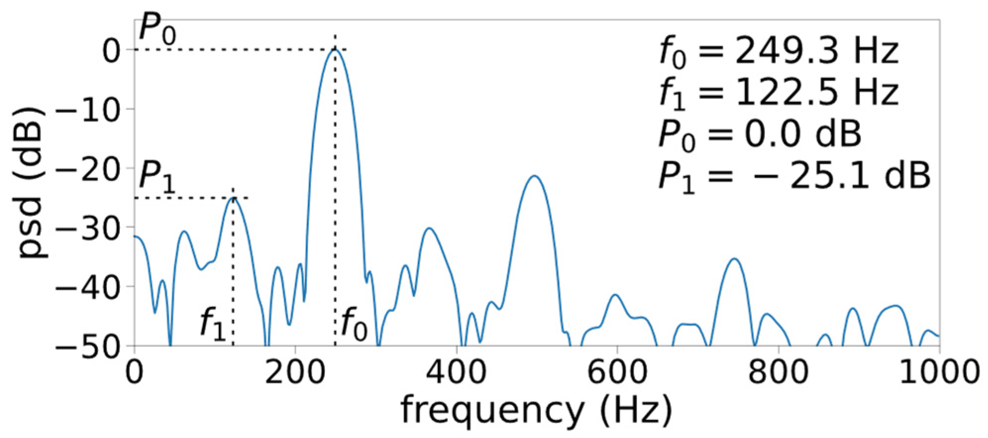
2.1. Tonal Frequency Selection Algorithm for Glottal Source Signals

The computation of the HDF and BI hinges on a proper strategy for selecting the two peaks, $f_0$ and $f_1$. The proposed approach is based on a periodogram, which is a nonparametric power spectral density (PSD) estimate. The key assumption of the algorithm is that the strongest spectral peak corresponds to the first harmonic of the voice signal (only if its harmonic structure is apparent). This is a reasonable assumption for a glottal source signal such as glottal area waveform. Note that this algorithm is not suitable for acoustic signals because the vocal tract effect can cause acoustic signals to violate this assumption.

2.1.1. Signal Preparation

For each full input signals, the temporal locations of the voiced segments are marked. In preparation, the input signal is first decimated (resampled) to form a narrowband signal, capturing at least two harmonics (e.g., $f_s=2000$ samples/second is sufficient for normal pitch around 100 to 250 Hz). This focuses the analysis on the low frequency contents and reduces the necessary computational effort. The marked voiced segments in the resampled signal are then broken into (possibly overlapped) short analysis windows, each containing $N$ voiced samples. In each window, these samples are linearly detrended to remove the dc component as well as a gradual drift. Let $\mathcal{X}=\left\{x_0, x_1, \dots ,x_{N-1}\right\}$ denote the set of the $N$ contiguous detrended samples $x_n$ in an analysis window.

2.1.2. Main Algorithm

The PSD of the detrended samples $\mathcal{X}$ is estimated with a windowing function with minimal sidelobe leakage. The use of such a windowing function is critical to avoid erroneously picking sidelobe peaks as real spectral peaks. Additionally, sufficient zero-padding is applied to obtain a denser representation of the underlying discrete-time Fourier transform. Let the estimated PSD $P_{xx}\left(f\right)$ as a function of frequency $f$ in Hz.

All spectral peaks in $P_{xx}\left(f\right)$ are identified with a simple peak-picking technique followed by quadratic peak interpolation. Let ${ℱ}_{\mathrm{all}}$ be the set of the frequencies of all the peaks. Note that ${ℱ}_{\mathrm{all}}$ includes all the local peaks, possibly including those of the noise and window sidelobe peaks. The first peak frequency is chosen at the global maxima:

$$\begin{array}{cc}{f}_0=\underset{f\in {ℱ}_{\mathrm{all}}}{\mathrm{argmax}}{P}_{xx}\left(f\right)& P_0=P_{xx}\left(f_0\right)\end{array}$$

(4)

Because $\mathcal{X}$ has been detrended, $f_0>0$ is guaranteed, thus $\mathsf{\gamma }$ is finite, as per (1).

Denoting the remaining peaks by ${ℱ}_1={ℱ}_{\mathrm{all}}\setminus \left\{f_0\right\}$, the next strongest peak is detected as a point of reference:

$$\begin{array}{cc}{f}_{\mathrm{ref}}=\underset{f\in {ℱ}_1}{\mathrm{argmax}}{P}_{xx}\left(f\right),& P_{\mathrm{ref}}=P_{xx}\left(f_{ref}\right)\end{array}$$

(5)

This reference peak is used to form a threshold to define a set of candidates for the second peak $f_1$:

$${ℱ}_{\mathrm{can}}=\left\{f:f\in {ℱ}_1, P_{xx}\left(f\right)>\rho P_{\mathrm{ref}},f>f_g\right\},$$

(6)

where $\rho$ is a relative threshold parameter and $f_g$ is a minimum frequency parameter to avoid selecting a spurious near-dc peak. Finally, the chosen candidate in ${ℱ}_{\mathrm{can}}$ is the one such that its HDF value is closest to 1.0:

$$f_1=\underset{f\in {ℱ}_{\mathrm{can}}}{\mathrm{argmin}}\left|1-\mathrm{HDF}\left(f\right)\right|.$$

(7)

Here, $\mathrm{HDF}\left(f\right)$ represents the HDF value computed from a given arbitrary $f$ by $\mathsf{\gamma }=f/f_0$ and (2). This selection criterion favors the biphonic case (in which the other fundamental frequency is closer to $f_0$) followed by subharmonic frequencies, then by the harmonic frequencies. For a Type-I voice, ${ℱ}_{\mathrm{can}}$ is expected to contain only the harmonic frequencies, while a Type-II voice may produce ${ℱ}_{\mathrm{can}}$ with both non-harmonic and harmonic frequencies. The selection strategy in (7) guarantees to pick non-harmonic frequencies if present.

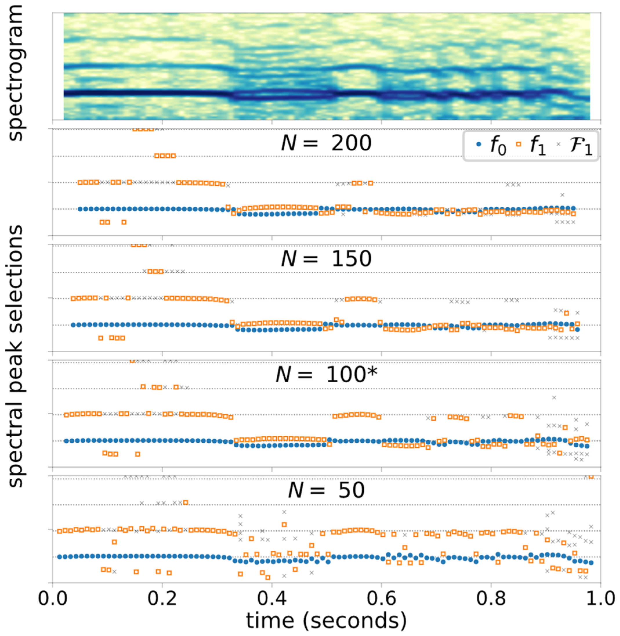
2.2. Experiment Configurations

A glottal area waveform (which is a sequence of numbers of glottal pixels per frame) of sustained /i/ phonation is obtained for each case and are prepared to $f_s=2000$ samples/second. See Appendix A for details of the source high-speed endoscopic data and how the waveforms were generated. Each signal is processed over a 100-sample (50-ms) sliding analysis window, offset by 10 samples (5 ms) at a time.

Table 3. Experiment Parameter Setup.

Name	Parameter	Value
Sampling rate	$f_s$	2000
Window Size	$N$	100 (50 milliseconds)
Window Offset	$N_{\mathrm{offset}}$	20 (10 milliseconds)
Window Function		Hamming
Number of PSD Samples	$N_{\mathrm{fft}}$	1024
${ℱ}_1$ Relative Threshold	$\rho$	1/4 (0.25)
Minimum $f_2$ frequency	$f_g$	25 Hz

summarizes the values chosen for all the analysis parameters. The Hamming windowing function is chosen as it provides a good tradeoff between spectral resolution and sidelobe suppression for a 50-millisecond window. The relative threshold parameter $\rho =1/4$ allows the PSD peaks that are –6 dB below the reference peak to be considered for $f_1$.

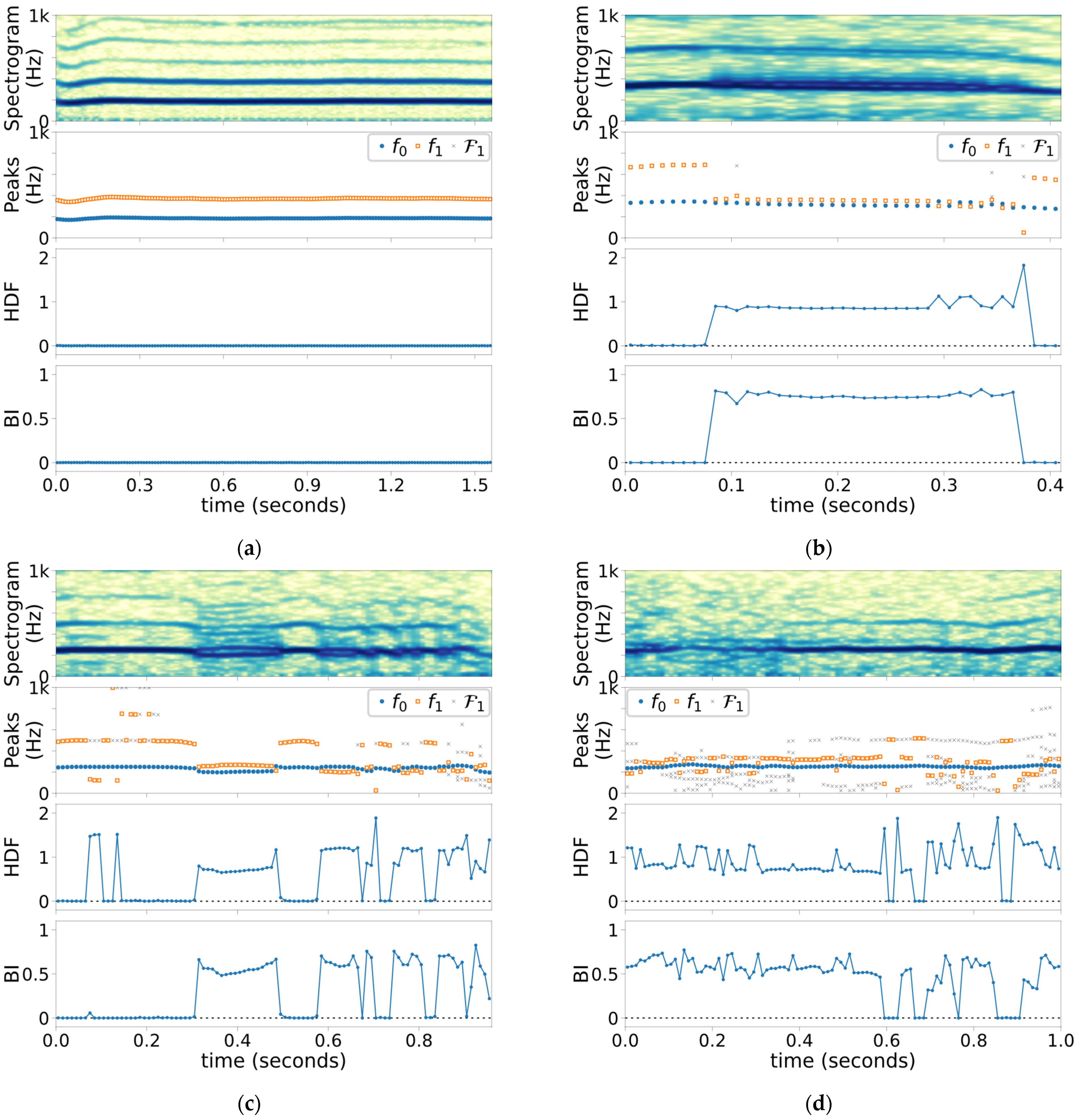
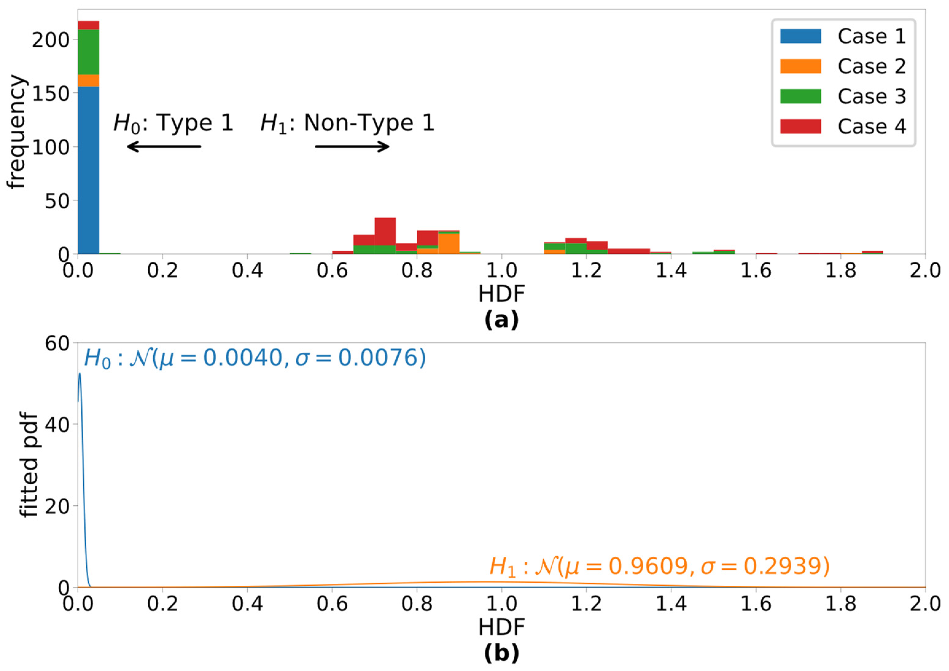
2.3. Case Study Samples and Study Outcomes

Four cases are chosen to illustrate the parameters’ response to various voice types and mid-phonation bifurcations, as shown in

Table 4. Descriptions of Cases Studied.

	Voice Description	# of Bifurcations	Notes
Case 1	Type I	0	No Pathology
Case 2	Types I + II	2	UVFP, Biphonia
Case 3	Types I + II	>10	Polyp, Biphonia + Subharmonics
Case 4	Types II + III	4	Polyp, $f_0$ mostly present throughout

. All cases are of female voice. The three cases with voice disorders (one case of unilateral vocal fold paralysis (UVFP) and two cases of polyp) exhibit mid-phonation bifurcations; Case 3 appears to have more than 10 observable bifurcations in 0.948 s. These pathological cases, as a result, have multiple signal types: all exhibit Types I and II; Case 4, in addition, exhibits Type-III behavior. For each case, the following short-term measurement outcomes are plotted: spectrogram, frequencies of the selected and considered peaks ($f_0$, $f_1$, ${ℱ}_1$), HDF, and BI.

Next, two additional experiments are conducted to observe the performance of the spectral peak selection algorithm as its parameters are varied, namely, the ${ℱ}_1$ threshold $\rho$ and the window size $N$. They are both tested with the Case 3 signal. The following four threshold values are considered: $\rho \in \left\{1/2, 1/4, 1/8, 1/16\right\}$. In decibels, they correspond to –3, –6, –9, and –12 dB below the second strongest spectral peak power. A more aggressive (lower) threshold setting is expected to increase the incorrect $f_1$ selection in the Type-I window. Additionally, four window sizes are considered: $N=$ 200 (100 ms), 150 (75 ms), 100 (50 ms), and 50 (25 ms). While a short window size is desirable for bifurcation detection, too short of a window causes the mainlobes of harmonic peaks to be too wide to distinguish them apart.

3. Results

Figure 2 shows the outcomes of the short-term analyses of the four cases under study, and Figure 3a shows the histogram of HDF measurements. All the analysis windows with their HDF values less than 0.1 (the first 2 bins) were perceptually identified to contain Type-I signals. Figure 3b illustrates the estimated conditional normal pdfs for the two detection hypotheses. Given these conditional pdfs, the false-alarm rate is chosen to be 0.01%, and the non-Type-I detection rate of the HDF-based detector is estimated as 99.9%.

Figure 4 illustrates the Case 3 spectral peak selection outcomes with varying threshold level $\rho$ settings, and Figure 5 shows the Case 3 spectral peak selection outcomes with varying window size, $N$. The color intensity of the spectrograms are shown in decibels with 50-dB dynamic range.

4. Discussion

4.1. Overall Impression of HDF and BI

The proposed HDF with the experiment configuration in Table 1 has demonstrated excellent ability to distinguish Type-I segments from others, as shown in Figure 2, corresponding well to visual cues that are present in the spectrograms. This includes both the normal voice in Case 1 as well as during the Type-I segments in the pathological cases. Visual observation of Figure 2 is confirmed by the HDF histogram in Figure 3, which illustrates a wide gap between Type-1 HDF values and those of other types. Further analysis of the histogram predicts the 99.9% detection rate of non-Type-I voice signal while fixing the false alarm rate at 0.01%. While this prediction is made with limited data, it still is a strong indication of the HDF’s ability to detect non-Type-I signals reliably.

The BI (and to lesser extent HDF) are expected to maintain a fixed level for each Type-II voicing mode. This is apparent in the three pathological cases, but most clearly in Case 2 (Figure 2b). After the bifurcation at $t=0.1$, the BI stays around 0.76 (which corresponds to the “7:8” attractor notation of Steinecke and Herzel [13]) until the next bifurcation at $t=0.37$. Towards the end of this period, the HDF jumps between 0.875 and 1.143, which are reciprocal of each other, due to near-equal spectral peaks, causing $f_0$ and $f_1$ to flipflop. This behavior is the reason to introduce the BI.

Case 3, whose acoustic signal is shown in Figure 1, exhibits numerous bifurcations. Its spectrogram in Figure 2c indicates the voice mostly switches between Type I and biphonic Type II. The HDF distinguishes Type-I and Type-II segments, including the momentary returns to the Type-I signal amid biphonic Type-II phonation in $t\in \left(0.6, 0.9\right)$ correctly. At the beginning and end, period-2 subharmonic voicing is present, and the insensitivity of the BI to the period-2 subharmonic is prevalent (as expected per Table 2).

Type-III voice is defined as random or chaotic, and Case 4 (Figure 2d) appears to have such behavior between $t=$ 0.1 and 0.4, as per visual inspection of the spectrogram, although the speaking fundamental frequency $F_0$ is observable throughout. As expected from the Type-III signal, the spectrum over this Type-III segment consists of many peaks, which gives an impression of randomness. Most notably, the number of candidates in ${ℱ}_1$ is substantially higher than the other cases, which is an indication of the consistent presence of noise-like disturbance. However, a closer inspection of the BI and the frequencies of the peaks suggests that there is a consistent undertone of 7:9 mode (BI = 0.56) and thus has a strong Type-II quality to it. Nonetheless, the expected higher variation of HDF and BI for the Type-III signal is apparent from the Case 4 results.

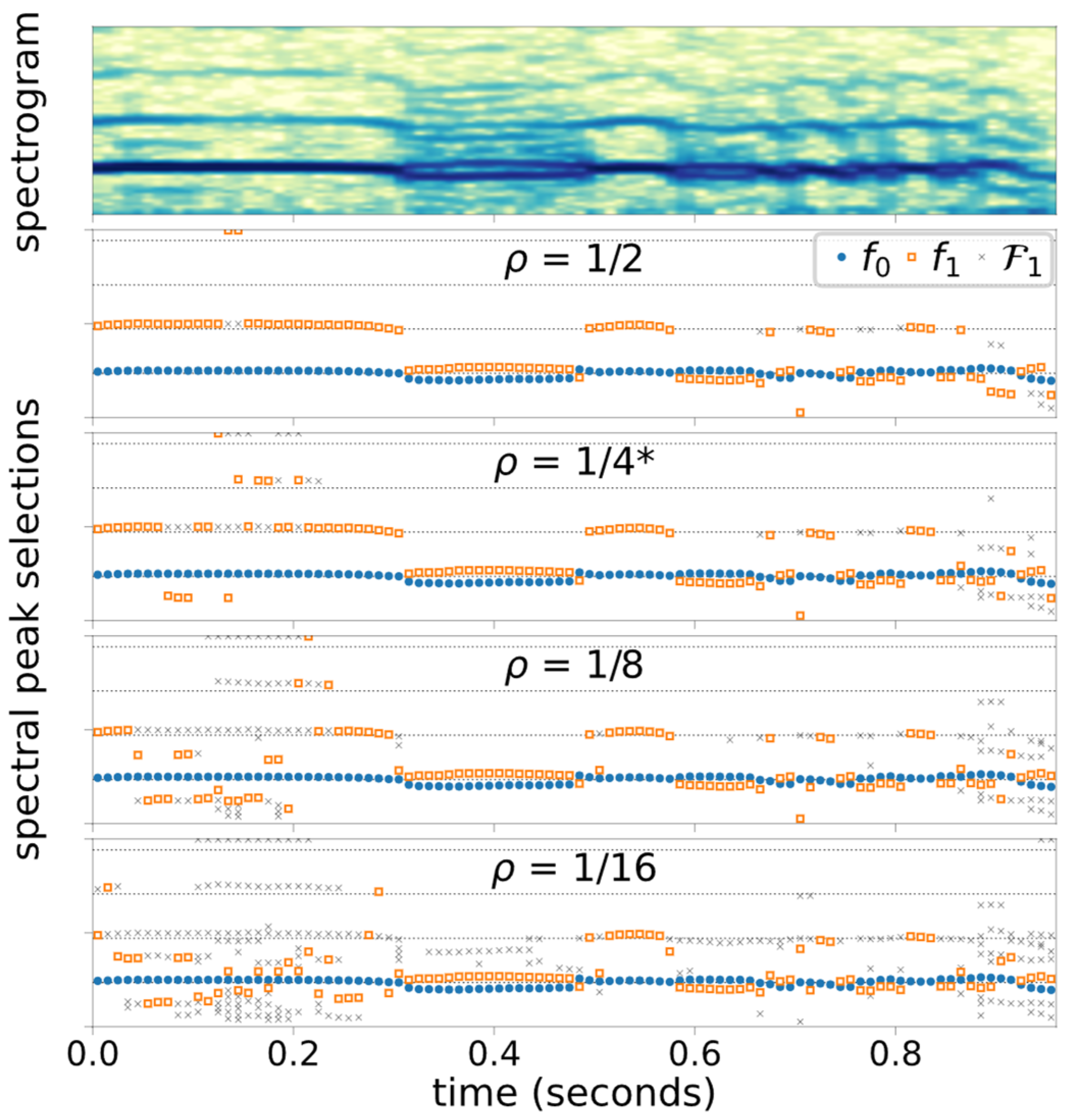
4.2. Sensitivity of HDF and the Proposed Frequency Selection Algorithm

The effectiveness of HDF and BI depends on the algorithm to select $f_0$ and $f_1$. The proposed periodogram-based algorithm has been shown to provide consistently accurate estimates to HDF and BI in the presented four cases. The configuration used (Table 1) has been carefully chosen for the four cases presented in this paper, and the results in Figure 4 and Figure 5 illustrate the considerations needed for the parameter selection process.

Figure 4 shows how the frequency selection process is affected by the relative threshold parameter $\rho$, which defines the $f_2$ candidate selection threshold relative to the second strongest peak in the spectrum. In general, more aggressive (lower) $\rho$ yields more candidate peaks, thus there is a higher likelihood of selecting non-harmonic peaks. With the base configuration ($\rho =1/4)$, the algorithm misses the presence of a weak-but-consistent period-doubling subharmonic present at the beginning, viz. $t\in \left(0,0.1\right)$. These subharmonic peaks are –25 dB below the $f_0$ peaks, as shown in Figure 6. By lowering the threshold ($\rho =1/8$ and $1/16$), these subharmonic peaks can be detected. However, lowering also causes the detection of non-harmonic peaks during the following segment at $t\in \left(0.1, 0.3\right)$, over which visual inspection of the spectrogram suggests Type-I voicing. This leaves us a question: How small of a subharmonic peak is considered perceptible?

The selection threshold $\rho$ for $f_1$ ought to be drawn based on the audibility of the signal component, which the spectral peaks represent. Orlikoff and Baken [30] suggest that the power of non-harmonic peaks of the Type-I signal must be at least an order of magnitude (or –10 dB) lower than that of the first harmonic. Under this guideline, the observed subharmonics in Figure 6 are weak enough to be ignored (–25 dB under the first harmonic). However, it may be too conservative as a –10 dB threshold leaves out the second harmonic, which is –20 dB below the first harmonic and may have perceptual relevance. Bergan and Titze [9] found that perception of roughness is consistently reported (albeit at a five-out-of-ten rating) above 20% amplitude modulation. The amplitude modulation effect that was tested in their study would introduce period-doubling subharmonics, but how the 20% figure translates to the relative power of subharmonic peaks was not reported. Future experimental study is necessary to identify the audible amount of subharmonics to solidify the peak detection requirement.

Another factor regarding the performance of the frequency selection algorithm is the analysis window length. There is a tradeoff between the frequency and time resolutions. A longer window enables detection of closer spectral peaks but blurs the location of a bifurcation (if present). Conversely, a change in time can be detected more precisely with a shorter window but with an expense of lost frequency resolution. Both cases are presented in Figure 5. During a consistently biphonic segment $t\in \left(0.3,0.5\right)$, the shortest window length ($N=50$) fails to detect the second fundamental frequency consistently due to the insufficient spectral resolution. Meanwhile, during the segment $t\in \left(0.6,1.0\right)$, in which the voice type switches rapidly, a wide window ($N\ge 100$) bridges over the transitions and reports biphonic frequencies throughout this segment. To determine the optimal window size for general use, further experimentation with additional signal samples is needed. Specifically, the algorithm and its configuration must be tested with a wider range of speaking fundamental frequencies, including male voice, with which biphonic frequencies are closer together by virtue of lower fundamental frequency.

4.3. Clinical Applications

The HDF and BI are short-term parameters, which are meant to be measured repeatedly over each voice sample. With the HDF ability to distinguish Type I and Type II/III, it could be used in the automation of spectrogram visual inspection for clinical assessment. Additionally, these measurements can be further processed to form objective parameters, which are potentially clinically useful indicators for voice quality.

The clinical value of HDF and BI measurements themselves (or their means over multiple windows) needs to be further investigated. These parameters are designed primarily to detect bifurcations, i.e., to observe the changes in their values in time. They, however, could be significant measures if different biphonic or subharmonic components in voice are perceived differently and found to be contributing to severity of voice quality; for example, period-doubling vs. period-tripling subharmonics and 2:3 biphonia vs. 3:5 biphonia. To the authors’ knowledge, there is no known related work in the literature.

What is likely to be perceivable, on the other hand, is the occurrence rates of non-Type-I voicing and of voice-type switching. This leads us to two viable objective parameters: amount of harmonically disturbed phonation and the rate of bifurcation. The former quantifies how much time during phonation the voice exhibited non-Type-I behavior, and the latter how often voice bifurcations occur. The cases in this paper demonstrated promising signs for the HDF to serve these objective parameters. The HDF of Type-I voice is tightly concentrated at zero. This allows reliable detection of non-Type-I short-term phonation, and therefore the HDF is an excellent basis to form an effective parameter to quantify the occurrence rate of non-Type-I voicing.

The alternate parameter, quantifying the occurrences of mid-phonation bifurcations, requires additional analysis: distinguishing the three phonation types and detecting changes within Type II. Both HDF and BI can contribute to this analysis. The HDF and BI measures in each phase-locked Type-II segment are drawn from a fixed set of values, as illustrated in Figure 2. As such, a transition to another Type-II mode is likely to introduce a discontinuity in the HDF or BI measures. To detect transition away from a biphonic segment, the BI is more a reliable solution than the HDF as the BI takes a unique value for each biphonic mode (2:3, 3:5, etc.). Detection of Type III can be achieved by monitoring the variation of the HDF (or BI) over several windows. Further development is required to better understand the implementational limitations, such as noise characteristics and measurements in the windows that bridge two distinctive modes. Additionally, a dedicated classifier for subharmonic periodicity would complement HDF and BI and strengthen bifurcation detection.

This paper focused on glottal source signals, specifically on the glottal area waveforms from high-speed videoendoscopic data. Other types of source signals, such as the electroglottogram, could use the same algorithm if the first harmonic is the most dominant harmonic. This condition is not satisfied by acoustic signals due to the vocal tract effect. Thus, extending the HDF to general voice signals, especially acoustic signals, requires a frequency selection algorithm that can identify the speaking fundamental frequency. With such an algorithm, the HDF concept can be extended to the assessment of voicing changes in connected speech, which is known to expose dysphonia more than sustained phonation [23].

5. Conclusions

This paper proposes short-term parameters: the harmonic disturbance factor (HDF) and the biphonia index (BI), both of which are based on the ratio of two tonal frequency contents in the voice signal. The HDF and BI are intended to distinguish Type-I signals from Type-II or Type-III signals. Four cases (one normal, three with pathology) are shown to illustrate the behavior of the measures against a wide range of voicing behaviors, and the HDF and BI have exhibited the intended outcomes. The preliminary analysis of the HDF-based detector of non-Type-I voice signals is also presented, reporting a 99.9% detection rate with fixed a 0.01% false-alarm rate. Potential applications of these parameters towards objective clinical assessment are suggested.

References

1. Bless, D.M.; Hirano, M.; Feder, R.J. Videostroboscopic evaluation of the larynx. Ear. Nose. Throat J. 1987, 66, 289–296. [Google Scholar] [PubMed]
2. Poburka, B.J.; Patel, R.R.; Bless, D.M. Voice-Vibratory Assessment with Laryngeal Imaging (VALI) form: Reliability of rating stroboscopy and high-speed videoendoscopy. J. Voice 2017, 31, 513.e1–513.e14. [Google Scholar] [CrossRef]
3. Titze, I.R. Workshop on Acoustic Voice Analysis: Summary Statement; National Center for Voice and Speech: Denver, CO, USA, 1994. Available online: http://www.ncvs.org/freebooks/summary-statement.pdf (accessed on 23 February 2021).
4. Jiang, J.J.; Zhang, Y.; McGilligan, C. Chaos in voice, from modeling to measurement. J. Voice 2006, 20, 2–17. [Google Scholar] [CrossRef] [PubMed]
5. Liu, B.; Polce, E.; Jiang, J. Application of local intrinsic dimension for acoustical analysis of voice signal components. Ann. Otol. Rhinol. Laryngol. 2018, 127, 588–597. [Google Scholar] [CrossRef]
6. Liu, B.; Polce, E.; Raj, H.; Jiang, J. Quantification of voice type components present in human phonation using a modified diffusive chaos technique. Ann. Otol. Rhinol. Laryngol. 2019, 128, 921–931. [Google Scholar] [CrossRef]
7. Liu, B.; Polce, E.; Jiang, J. An objective parameter to classify voice signals based on variation in energy distribution. J. Voice 2019, 33, 591–602. [Google Scholar] [CrossRef] [PubMed]
8. Liu, B.; Raj, H.; Klein, L.; Jiang, J.J. Evaluating the voice type component distributions of excised larynx phonations at three subglottal pressures. J. Speech Lang. Hear. Res. 2021, 64, 1447–1456. [Google Scholar] [CrossRef]
9. Bergan, C.C.; Titze, I.R. Perception of pitch and roughness in vocal signals with subharmonics. J. Voice 2001, 15, 165–175. [Google Scholar] [CrossRef]
10. Herzel, H.; Knudsen, C. Bifurcations in a vocal fold model. Nonlinear Dyn. 1995, 7, 53–64. [Google Scholar] [CrossRef]
11. Zañartu, M.; Mehta, D.D.; Ho, J.C.; Wodicka, G.R.; Hillman, R.E. Observation and analysis of in vivo vocal fold tissue instabilities produced by nonlinear source-filter coupling: A case studya). J. Acoust. Soc. Am. 2011, 129, 326–339. [Google Scholar] [CrossRef] [PubMed] [Green Version]
12. Behrman, A.; Baken, R.J. Correlation dimension of electroglottographic data from healthy and pathologic subjects. J. Acoust. Soc. Am. 1997, 102, 2371–2379. [Google Scholar] [CrossRef]
13. Steinecke, I.; Herzel, H. Bifurcations in an asymmetric vocal-fold model. J. Acoust. Soc. Am. 1995, 97, 1874–1884. [Google Scholar] [CrossRef] [PubMed]
14. Berry, D.A.; Herzel, H.; Titze, I.R.; Story, B.H. Bifurcations in excised larynx experiments. J. Voice 1996, 10, 129–138. [Google Scholar] [CrossRef]
15. Mergell, P.; Herzel, H.; Titze, I.R. Irregular vocal-fold vibration—High-speed observation and modeling. J. Acoust. Soc. Am. 2000, 108, 2996–3002. [Google Scholar] [CrossRef] [PubMed]
16. Boersma, P.; Weenink, D. Praat: Doing Phonetics by Computer [Computer program]. Version 6.1.38. Available online: http://www.praat.org/ (accessed on 4 February 2021).
17. Hermes, D.J. Measurement of pitch by subharmonic summation. J. Acoust. Soc. Am. 1988, 83, 257–264. [Google Scholar] [CrossRef] [PubMed]
18. Sun, X. Pitch determination and voice quality analysis using Subharmonic-to-Harmonic Ratio. In Proceedings of the 2002 IEEE International Conference on Acoustics, Speech, and Signal Processing, Orlando, FL, USA, 13–17 May 2002; Volume 1, pp. I-333–I-336. [Google Scholar] [CrossRef]
19. Herbst, C.T. Performance evaluation of subharmonic-to-harmonic ratio (SHR) computation. J. Voice 2021, 35, 365–375. [Google Scholar] [CrossRef] [PubMed]
20. Deliyski, D. Acoustic Model and Evaluation of Pathological Voice Production; EUROSPEECH: Berlin, Germany, 1993. [Google Scholar]
21. Aichinger, P.; Roesner, I.; Schneider-Stickler, B.; Leonhard, M.; Denk-Linnert, D.M.; Bigenzahn, W.; Fuchs, A.K.; Hagmüller, M.; Kubin, G. Towards Objective Voice Assessment: The Diplophonia Diagram. J. Voice 2017, 31, 253.e17–253.e26. [Google Scholar] [CrossRef]
22. Awan, S.N.; Awan, J.A. A two-stage cepstral analysis procedure for the classification of rough voices. J. Voice 2020, 34, 9–19. [Google Scholar] [CrossRef] [PubMed] [Green Version]
23. Kramer, E.; Linder, R.; Schönweiler, R. A study of subharmonics in connected speech material. J. Voice 2013, 27, 29–38. [Google Scholar] [CrossRef]
24. Jiang, J.; Zhang, Y. Nonlinear dynamic analysis of speech from pathological subjects. Electron. Lett. 2002, 38, 294–295. [Google Scholar] [CrossRef]
25. Jiang, J.J.; Zhang, Y.; Ford, C.N. Nonlinear dynamics of phonations in excised larynx experiments. J. Acoust. Soc. Am. 2003, 114, 2198–2205. [Google Scholar] [CrossRef] [PubMed]
26. Awan, S.N.; Roy, N.; Jiang, J.J. Nonlinear dynamic analysis of disordered voice: The relationship between the correlation dimension (D2) and pre-/post-treatment change in perceived dysphonia severity. J. Voice 2010, 24, 285–293. [Google Scholar] [CrossRef] [PubMed]
27. Lopes, L.W.; Vieira, V.J.D.; Costa, S.L.d.N.C.; Correia, S.É.N.; Behlau, M. Effectiveness of recurrence quantification measures in discriminating subjects with and without voice disorders. J. Voice 2020, 34, 208–220. [Google Scholar] [CrossRef] [PubMed]
28. Vieira, V.J.D.; Costa, S.C.; Correia, S.L.N.; Lopes, L.W.; Costa, W.C.d.; de Assis, F.M. Exploiting nonlinearity of the speech production system for voice disorder assessment by recurrence quantification analysis. Chaos Interdiscip. J. Nonlinear Sci. 2018, 28, 085709. [Google Scholar] [CrossRef] [PubMed]
29. Neubauer, J.; Mergell, P.; Eysholdt, U.; Herzel, H. Spatio-temporal analysis of irregular vocal fold oscillations: Biphonation due to desynchronization of spatial modes. J. Acoust. Soc. Am. 2001, 110, 3179–3192. [Google Scholar] [CrossRef] [Green Version]
30. Baken, R.J.; Orlikoff, R.F. Clinical Measurement of Speech and Voice, 2nd ed.; Singular: San Diego, CA, USA, 2000. [Google Scholar]
31. Ikuma, T.; Kunduk, M.; McWhorter, A.J. Objective quantification of pre and post phonosurgery vocal fold vibratory characteristics using high-speed videoendoscopy and a harmonic waveform model. J. Speech Lang. Hear. Res. 2014, 57, 743–757. [Google Scholar] [CrossRef] [PubMed]
Figure 1. Snapshots of acoustic signal with mid-phonation bifurcation. At t 0 = 0.2 , the voice mostly presents Type-I behavior. It is, however, preceded by a Type-II mode with substantial subharmonics at t 0 = 0.1 and is then followed by Type-II voice with strong biphonia at t 0 = 0.3 . Another mode of biphonia occurs later at t 0 = 0.7 : (a) time-domain plots each over 100-ms window; (b) normalized power spectral density estimates (periodogram with Hamming window; only showing below 1 kHz, range −50 to 0 dB) in decibel scale. Vertical dotted lines indicate the estimated harmonic frequencies by Praat’s pitch estimator [16].
Applsci 11 05469 g001
Figure 2. Spectrograms (color intensity range: 50 dB), detected f 0 and f 1 peak frequencies and f 1 candidates in 1 , HDF’s, and BI’s of (a) Case 1 (Type I), (b) Case 2 (Types I and II), (c) Case 3 (Types I and II), and (d) Case 4 (Types I, II, and III).
Applsci 11 05469 g002
Figure 3. (a) Histogram of the HDF values of all four cases and (b) fitted conditional normal pdfs for Type-I signals ( H 0 ) and non-Type-I signals ( H 1 ).
Applsci 11 05469 g003
Figure 4. Case 3 Spectrogram and peak selection outcomes computed at four different thresholds, ρ . Horizontal grid lines approximate the harmonic frequencies. * indicates the base configuration.
Applsci 11 05469 g004
Figure 5. Case 3 Spectrogram (with N = 100 ) and peak selection outcomes computed with four different window sizes, N . Horizontal grid lines approximate the harmonic frequencies. * indicates the base configuration. (Time axes is shifted from other Case 3 plots for alignment.).
Applsci 11 05469 g005
Figure 6. Case 3 periodogram at t = 0.075 (7th window).
Applsci 11 05469 g006