1. Introduction
The design of robotized work cells or lines is a complex multidisciplinary task that is influenced by many external factors and conditions. During the designing process, it is necessary to make many decisions that greatly affect the resulting performance of the workplace and its properties, including the cycle time, velocity of individual parts, dynamic effects, vibrations, lifetime, ground area, and energy consumption.
Crucial for the design of a robotic cell is the selection of an appropriate industrial or collaborative robot and its placement in relation to other subsystems. The length of the designing stage of robotic cells is still shortening, which leads to the copying of existing layouts of workplaces with similar parameters and their adaptation to the actual requirements.
Any type of advanced optimization is almost impossible in this approach. However, this is the phase where it is possible to achieve some interesting savings of energy consumption, ground area, or the lifetime of some systems. The recent progress in complex simulation tools, such as Tecnomatix, Matlab—Robotics System Toolbox, CoppeliaSim (V-Rep), Gazebo, and Webots; methods for the creation of digital twins of the designed robotized workplace; and whole manufacturing lines [
1] open up new room for the realization of complex multicriteria optimizations in the early stages of design.
Optimizations of robotized workplaces to achieve the reduction of running costs are currently mostly realized in systems that are already in operation. These typically include modifications of the end-point trajectory according to a chosen criterion, such as the manipulation time [
2,
3] or the overall productivity and running costs of the robot [
4].
The optimization of the kinematic properties of the manipulator movement can also lead to the reduction of torques in individual joints and, thus, also the reduction of the overall energy consumption. For example, the authors in [
5] used interval analysis to find the global minimum jerk trajectory of a robot manipulator in a joint space using cubic splines, resulting in a smoother and vibration-free robot movement.
A similar approach was proposed in [
6], where the objective function included not only the integral of the squared jerk values but also the total execution time of the trajectory. The authors in [
7] used the 12-phase sine profile for trajectories of a fast-moving robot, which leads to a more stable and accurate movement without sudden changes of torques, albeit at the cost of a slightly higher overall energy consumption. Trajectory optimization with the single goal of cycle time reduction using the chicken swarm optimization (CSO) method was described in [
8].
Another optimization goal is the reduction of the workplace layout size [
9] because the usable area of the factory building is extremely valuable. There are also some methods for the multicriteria optimization of robotic work cells or lines for energy consumption—even for lines with up to 12 robots, based on the Gurobi simplex method [
10]. Another method of multi-robot cell optimization for time and energy reduction using a custom mechatronic model of the robots in Modelica/Dymola was described in [
11]. The authors in [
12] proposed a methodology for assembly line energy consumption optimization based on the implementation of energy-optimal trajectories, and, in [
13], this method was improved by modification of the actuator brake release time for additional energy consumption reduction.
A systematic methodology for the on-site identification and energy-optimal path planning of an industrial robot is presented in [
14] with a focus on a specific type of ABB industrial robot. Improved robot programming reduced the energy consumption compared to the built-in controller routines by up to 4%.
Further improvements and torque reduction for a robotized work cell can also be achieved by modification of the position and orientation of the robot base in relation to the optimized trajectory [
15]. This can be interesting, especially for applications where it is not possible to modify the end-point trajectory and velocity for technological reasons (the application of adhesives, edging, welding, etc.). In these cases, it is necessary to create a complex simulation model—a digital twin of the workplace [
16,
17] and perform a multicriteria optimization.
The Concept of Robot Wear
Gearboxes are often mentioned as the component that is frequently responsible for a failure of rotary machines [
18], including industrial robots [
19]. The most critical components of a gearbox are the gears and bearings. The deterioration of a gear appears at the teeth [
20,
21], harmonic drive gears are damaged by fatigue fractures [
22], and bearings are typically subjected to failures at the rolling elements or the inner or outer race [
21]. The damage accumulates over time and is caused mainly by load (forces and velocity) [
23,
24], high temperature [
25], bad lubrication [
26], or manufacturing defects. The performance, accuracy, and lifetime of a robot relies on the good condition of these critical components [
27].
The authors in [
28] proposed a method for estimating the wear of a robot by monitoring the temperatures in the joints, while [
29] suggested a more complex solution, where other parameters are also monitored in order to predict the lifetime of a multi-component system. Other common properties monitored to predict the lifetime of a machine include vibrations and noise [
21]. A generic framework for predictive maintenance based on simulation models with degradation curves discovered from real data was proposed in [
27]. Our approach, on the contrary, attempts to minimize wear by the use of a quite simple simulation in the design stage of a robotized workplace instead of monitoring an already existing one.
As mentioned above, the gearbox in the robot manipulator joint can be considered the most important source of the wear of the joint. The electric motor in the joint is subject to deterioration as well [
30]. As far as the above-mentioned sources of wear are concerned, the most important is the load combined with movement velocity, because a higher velocity creates higher temperatures. This applies to both the gearbox and the motor. The influence of bad lubrication or manufacturing defects are almost impossible to anticipate or even simulate and, thus, are not considered in this work.
A typical robot joint contains structural bearings that provide the mutual rotational movement of the joints. However, obtaining the values of the reacting forces required to calculate the wear of these bearings is not an easy task, even when using a dynamic simulation. This requires an exact simulation model of the robot with a detailed representation of the inner parts and mechanisms, accurate values of the mass properties, acceptably realistic values of the friction coefficients, and a good dynamic simulation engine. Although it is usually possible to obtain 3D models of commercially available industrial and collaborative robots, and sometimes even simulation models prepared for common simulation systems, these models typically are simplified and do not contain the inner mechanisms of the arms.
On the other hand, wear of the gearbox and motor can be expressed as torque that the motor must generate (and that the gearbox must transfer to the joint) over some trajectory of motion. These values depend on physical quantities that are much easier to obtain from a simulation—the overall path of motion (kinematics) and the required driving torque required to achieve the given acceleration (dynamics).
The hypothesis of our research is that the lifetime of a robot in a robotized workplace can be improved in the design stage by designing the workplace (namely the location of the robot) in such a way to ensure lower wear of the robot joints.
2. Materials and Methods
To determine the optimal placement of a robot manipulator within a robotic cell with the goal of reducing and balancing joint wear, it is necessary to propose a suitable optimization criterion, the whole optimization process, and an experiment to verify the results.
2.1. Optimization Criterion
In this work, we consider only the wear of the robot drive chain (see the previous section). We will also restrict the following notation to rotational joints (which are much more common than translational joints in robotics) and to six degrees of freedom (the most common number in robotics); however, the principles can be applied in general.
An industrial or collaborative robot in a robotized workplace usually performs a limited set of movements. Typically, there is a given trajectory that the robot end-point should follow during the work cycle, and the robot joints are controlled using inverse kinematics to adhere to this trajectory. The idea of wear being caused by a torque acting over a trajectory corresponds with the concept of mechanical work, which can be expressed as
where
is the magnitude of the torque vector,
is the angle of rotation about the vector representing the joint axis, and
and
are the starting and ending angles of rotation, respectively.
The integral (
1) is path-dependent and the mechanical work is defined as the change of energy. Thus, if we assume
, which is true for a closed-loop trajectory of the robot end-point (all individual joints have to start and end in the same angle of rotation), the resulting value of
W would always be equal to zero. It is, thus, more convenient to express mechanical work as the integral of mechanical power over time
where
is the angular velocity of motion and
and
are the starting and ending time, respectively. However, this integral (
2) is still path-dependent, and the calculation would result in
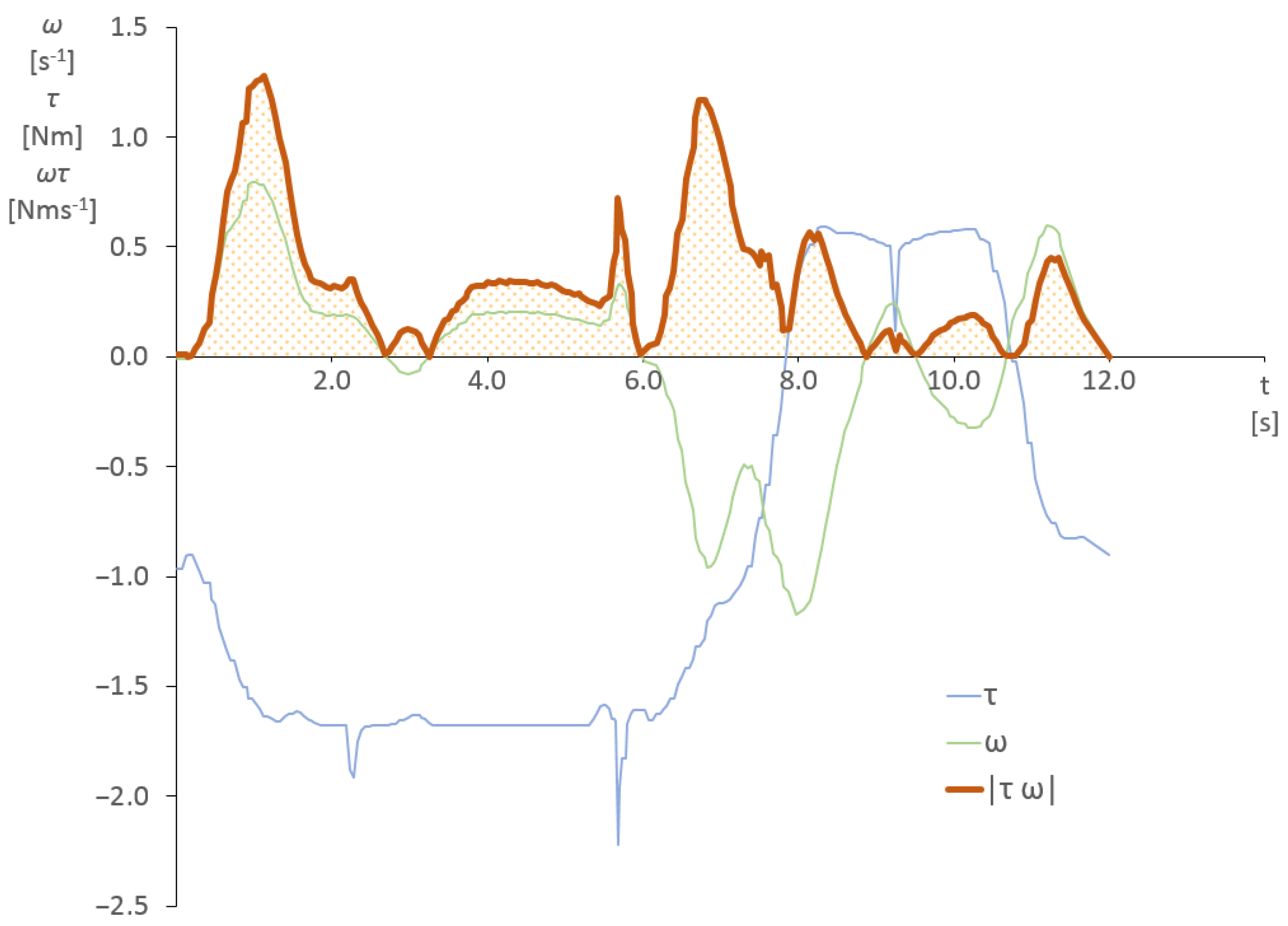
. Thus, it is necessary to introduce the absolute value of both the torque and the angular velocity
which allows us to calculate the work over the whole trajectory, while in fact, considering the trajectory divided into segments separated by the change of direction of movement or the change of the sign of
. This modification moves away from the concept of the conservation of energy toward the concept of wear caused by mechanical work. The idea is that the drive chain of a robot joint is worn down even when the torque is negative (the motor is actively braking) or when the angle of rotation is decreasing or moving back.
The simulation is numerical with a definitive value of
(simulation step size) instead of
. Therefore, the integral (
3) is replaced by a sum
where
is the simulation step,
is the instant torque, and
is the instant angular velocity in the
i-th simulation step. The mathematical meaning of the value
W is shown in an example in
Figure 1.
The value of W was calculated individually for each joint over the whole robot trajectory, yielding for the most common number of 6 degrees of freedom.
We attempted to optimize two factors:
Therefore, it is necessary to consider the values
together. However, the joints of a robot manipulator are typically not equal from the mechanical point of view, and their capabilities are different—the lower joints are larger and stronger, and the joints near the end-effector are lighter. The same magnitude of
W could, in reality, mean much higher stress and wear for a smaller joint than for a larger one. We, therefore, introduce a variable called the relative wear factor
, which is calculated by normalizing the individual
values
where
is the joint number,
is the maximal permissible torque, and
is the maximal angular velocity of the
j-th joint (both values are specified by the manufacturer of the robot).
To minimize the overall wear of the robot, we chose to use the arithmetic mean of the relative wear factors of all joints and to find the minimal value of this mean,
and balance is achieved by finding the minimal value of the standard deviation
The chosen fitness function (optimization criterion)
places the same weight on both these factors; therefore,
2.2. Optimization Process
The proposed method requires a simulation model capable of evaluating the movement of a robot manipulator through a given end-point trajectory while computing the values of joint angles and torques in individual time steps. This is possible, for example, in the popular robotic simulation system CoppeliaSim (formerly known as V-Rep), which was also chosen for our work.
The scripting capability of CoppeliaSim allows programming a robot’s end-point movement through a given trajectory and time, and the built-in physics engine (i.e., Bullet 2.78) is able to check for collisions and evaluate joint torque values. The inverse kinematics (IK) are calculated using the integrated pseudoinverse IK solver. The CoppeliaSim API (Application Programming Interface) framework (RemoteAPI) can be used to remotely configure the simulation, which, in our case, includes particularly the process of changing the robot placement relative to the trajectory, as we are trying to determine the optimal placement of the robot. A custom application was written in Visual C++ for this purpose.
Due to the long simulation times in CoppeliaSim, especially in the cases when the IK calculation fails (the robot cannot reach some parts of the given trajectory), all valid positions of the robot relative to the given trajectory were pre-calculated in the C++ application and CoppeliaSim was used only to calculate the fitness function value in those positions. The valid locations were found using a simple kinematic simulation inside the C++ application, which can quickly verify the ability of the robot to fulfill a given task from the specific location, including collision checking.
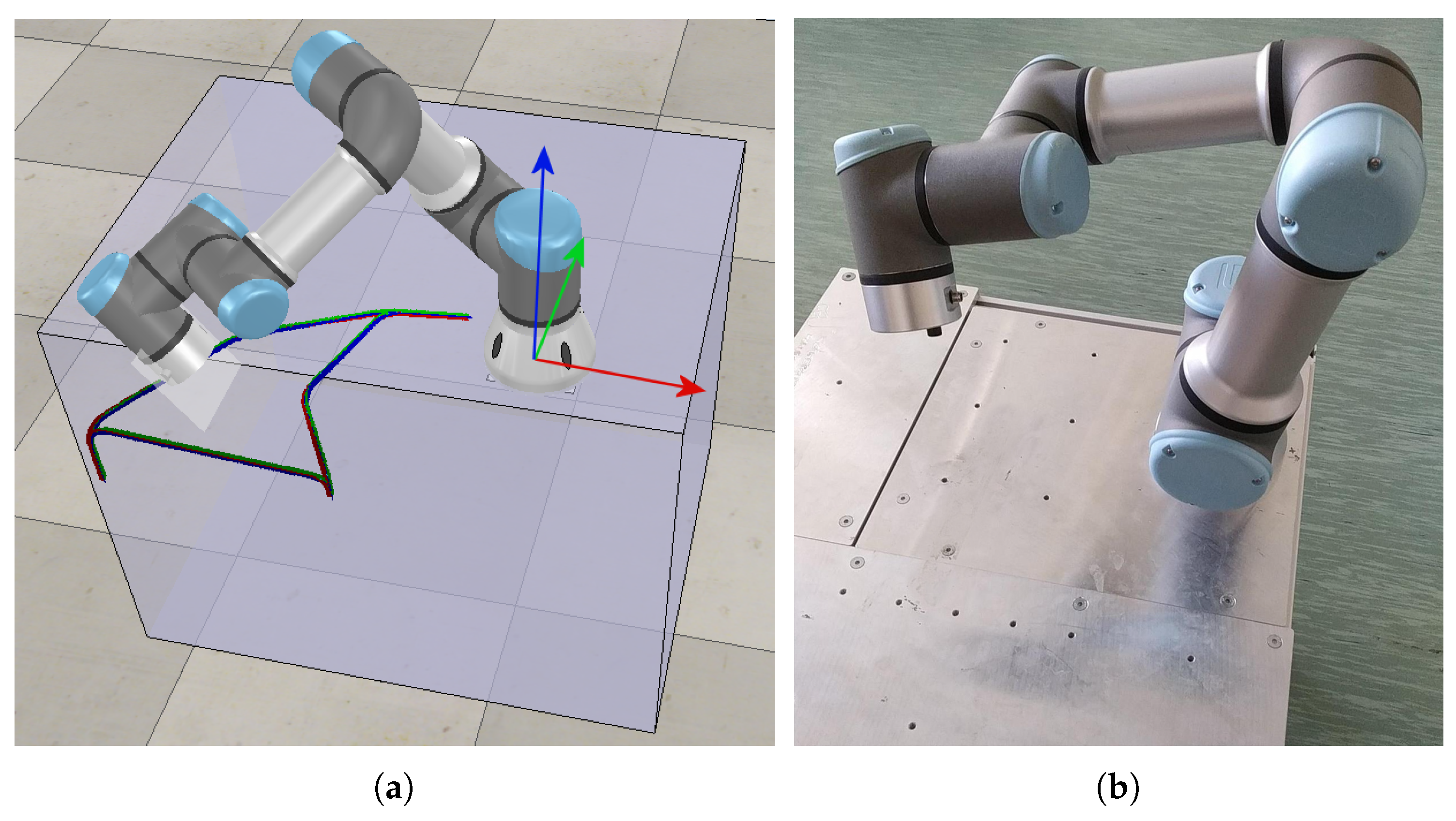
The search space is represented as a discrete 3-dimensional grid with the spacing in all three dimensions equal to
s = 0.03 m. The system returns the valid robot positions as a list of points, where each point represents the location of the center of the robot base (see the coordinate system in
Figure 2a) in the workspace. Verification of the whole robot trajectory in this simulation system took approximately 1800-times less time than the same task in CoppeliaSim, and invalid robot locations were discarded even faster.
For the reproducibility of the research, this supplementary custom simulation system is not necessary, as its main purpose is simply to shorten the overall simulation time. However, it is necessary to have an external application or a script in CoppeliaSim that successively places the robot in the locations from the above-mentioned search space (grid), executes the CoppeliaSim simulation, and calculates and stores the results.
The reason for choosing a 3-dimensional grid for the potential locations of the robot base instead of a 2-dimensional plane (representing the factory floor) is that the proposed method is intended to be as general as possible, and limiting the search to a 2-D grid could likely miss some interesting solutions. In reality, robots are commonly mounted on a stand, table or a console; therefore, the height of the robot can be chosen. However, the results can be easily limited to, for example, a 2-dimensional plane, if the actual application requires such a limit.
2.3. Experiment Setup
The proposed method was demonstrated and verified on a Universal Robots UR3 collaborative robot with 6 degrees of freedom (see
Figure 2), first in a CoppeliaSim simulation configured according to the previous chapter, and finally also on a real physical robot. The values of the maximal allowed joint torque
and joint angular velocity
(
5) for the UR3 robot are listed in
Table 1.
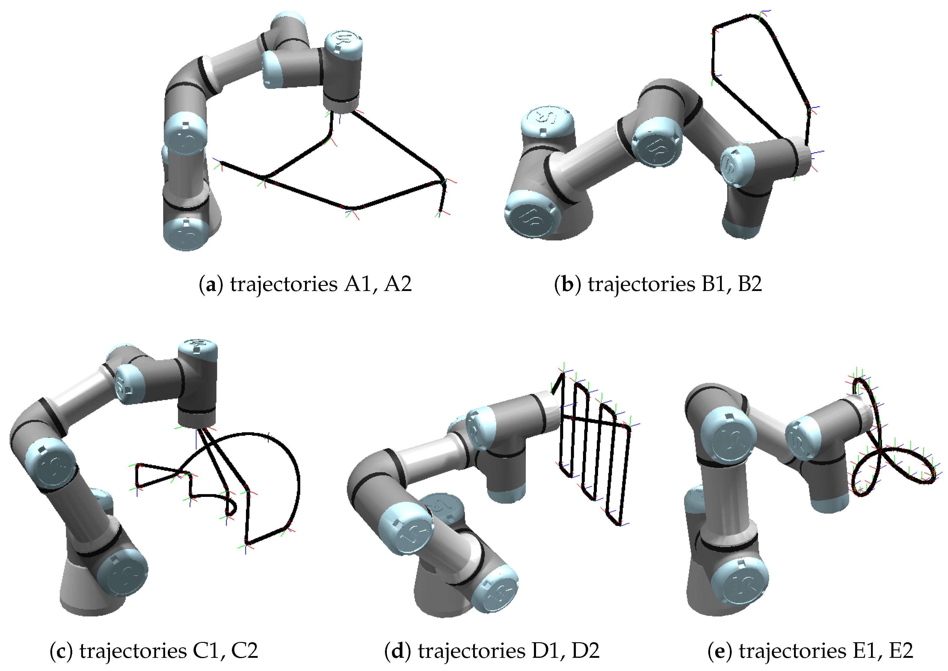
Five testing movement paths of the robot end-point were demonstrated, each in two variants with different velocities of the end-point (0.1 and 0.2 m/s), giving a total number of ten trajectories labeled A1, A2, B1, B2, …, E2; where A–E is the path type, 1 stands for 0.1 m/s, and 2 stands for 0.2 m/s.
The trajectories are a combination of real use-cases and artificially created simple trajectories that contain various elements (linear segments of different lengths, circle arcs, sections with frequent speed, direction changes, etc.), see
Figure 3. Various velocities of the end-point cause a difference in the solution of possible robot base locations, because every robot has some velocity limits for individual joints (see
Table 1), and they also represent different cases regarding the proposed wear factor calculation.
The selected trajectories were of a smaller size, and there were no obstacles in the environment (except for the table that the robot was mounted onto), which leads to a larger number of different valid robot locations relative to the trajectory and, thus, also a larger data set of results.
The chosen robot UR3 is a small robot with a reach of only 500 mm and although using larger trajectories combined with several obstacles in the environment would be possible, the valid locations of the robot would be very limited and it would be difficult to make a statistical evaluation. In general, the proposed optimization method does not depend on the size of the trajectory. A longer trajectory, requiring a longer time to traverse, would produce larger values of the discrete integral (
4); however, this is true for all robot locations relative to the particular trajectory, and thus the optimization remains valid.
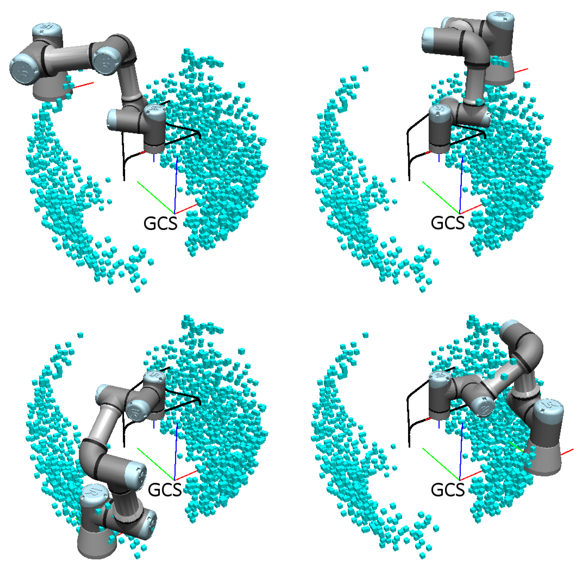
In a real case, the simulation model would have to contain also all collision objects in the workplace, which could limit the valid robot locations considerably—the principle of the method is, however, still applicable. The concept of choosing the robot location is demonstrated on
Figure 4 for the trajectory A1. The figure shows the grid of valid robot locations—each blue point represents a possible position of the robot base; the robot is able to reach the whole trajectory from each of these valid locations. For better clarity, the robot is shown in several selected locations.
3. Results
For each of the ten trajectories, the values of
(
5), and then
(
8) were calculated based on the CoppeliaSim simulation for each particular possible robot location in the grid. The important values are summarized in
Table 2, particularly the lowest fitness function value
in the best robot location, which should, thus, be the selected location for the robot, provided it is physically possible. The table also shows the percentage of improvement that the best location offers compared to the worst location,
which theoretically represents the greatest possible improvement in robot wear reduction. If we consider a random robot location versus the best one, the average improvement can be calculated compared to the average value
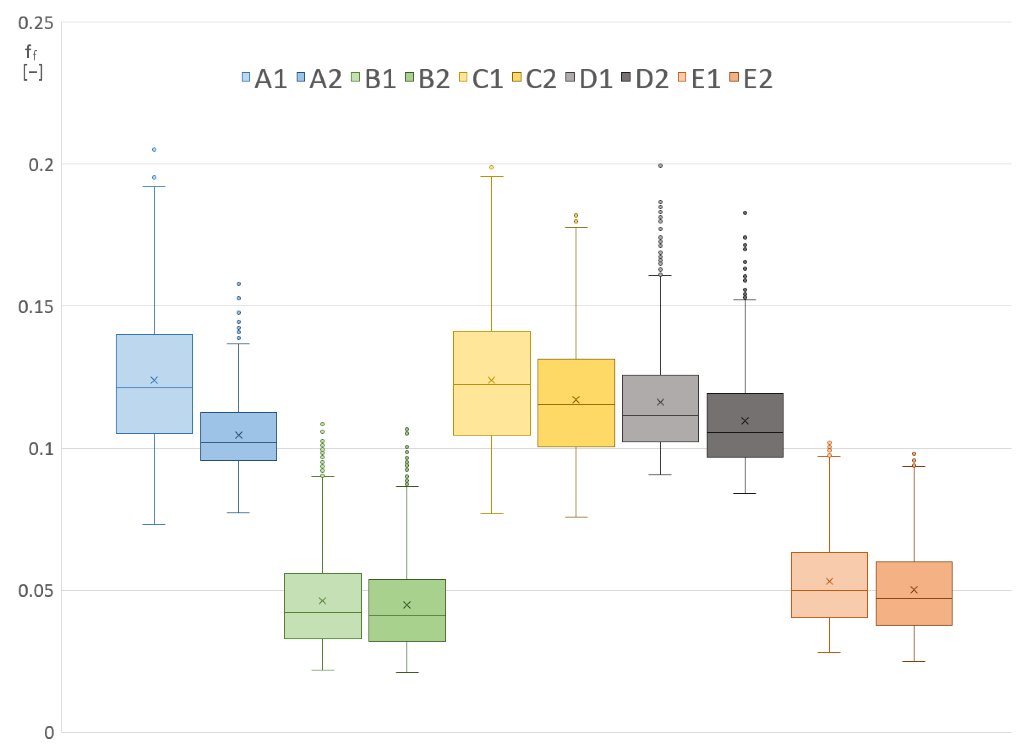
Figure 5 shows the distribution of
values in all possible robot locations for each trajectory in the form of a standard box-plot diagram. The height of each shaded rectangle represents the interquartile range (third quartile minus first quartile), which indicates that 50% of all
values lie inside the rectangle. The small circles in each column represent the outliers—the topmost one corresponds to the worst location with
.
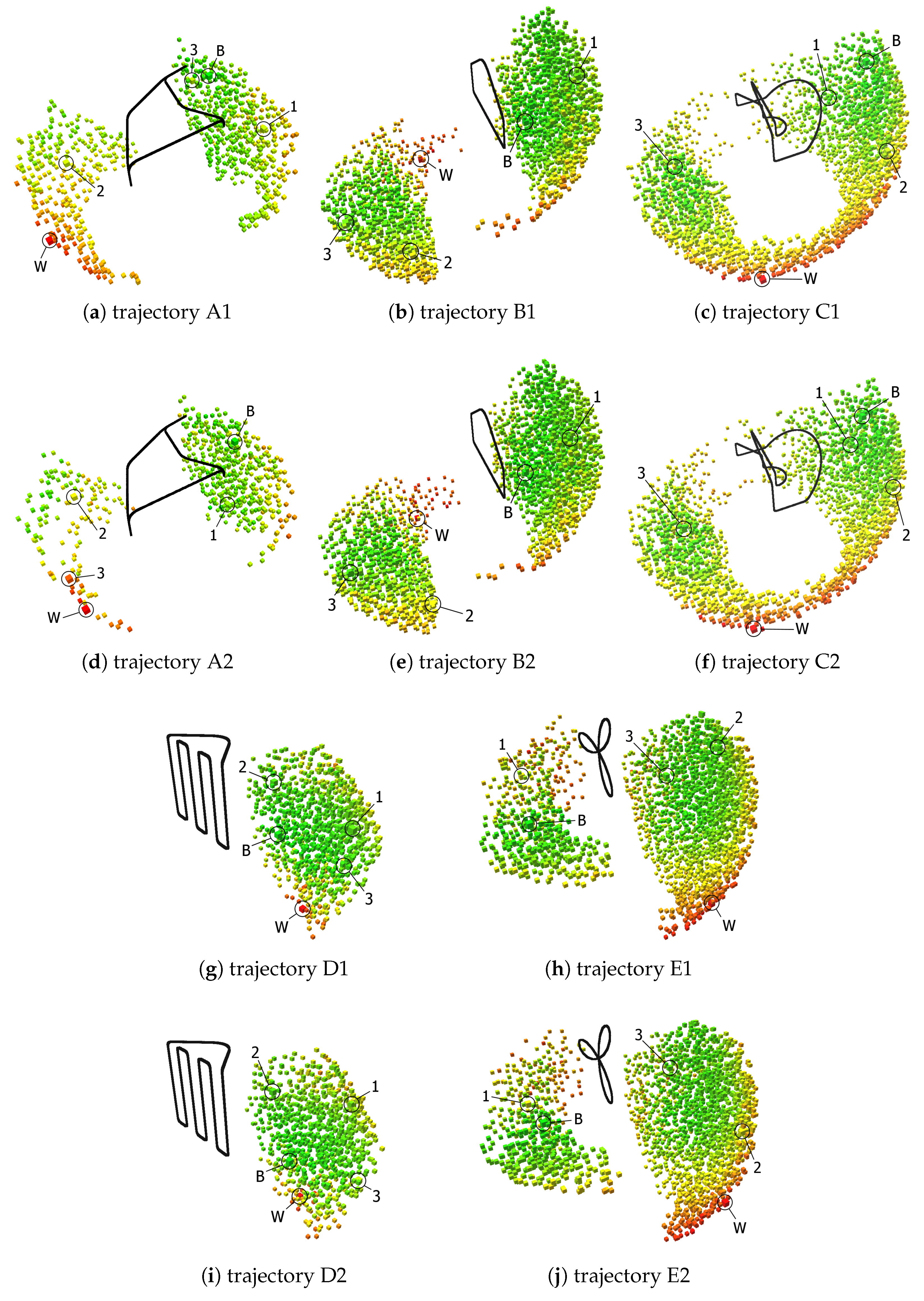
Arrangements of the robot locations in the 3D space around the corresponding trajectories are displayed in
Figure 6—the color coding indicates the
values using the gradient red–yellow–green, where green is the best location (
), and red is the worst (
). This image also shows the positions of the best (“B”), worst (“W”), and three other robot locations (“1”, “2”, and “3”) that will be used later in the experiments on a real robot. Note that the small cubes rendered in
Figure 6 as a visual representation of the possible robot locations are shifted away from the ideal grid positions by a small random offset (less than half the grid spacing). This is to achieve better visual clarity by preventing moiré patterns and reducing the concealment of more distant cubes.
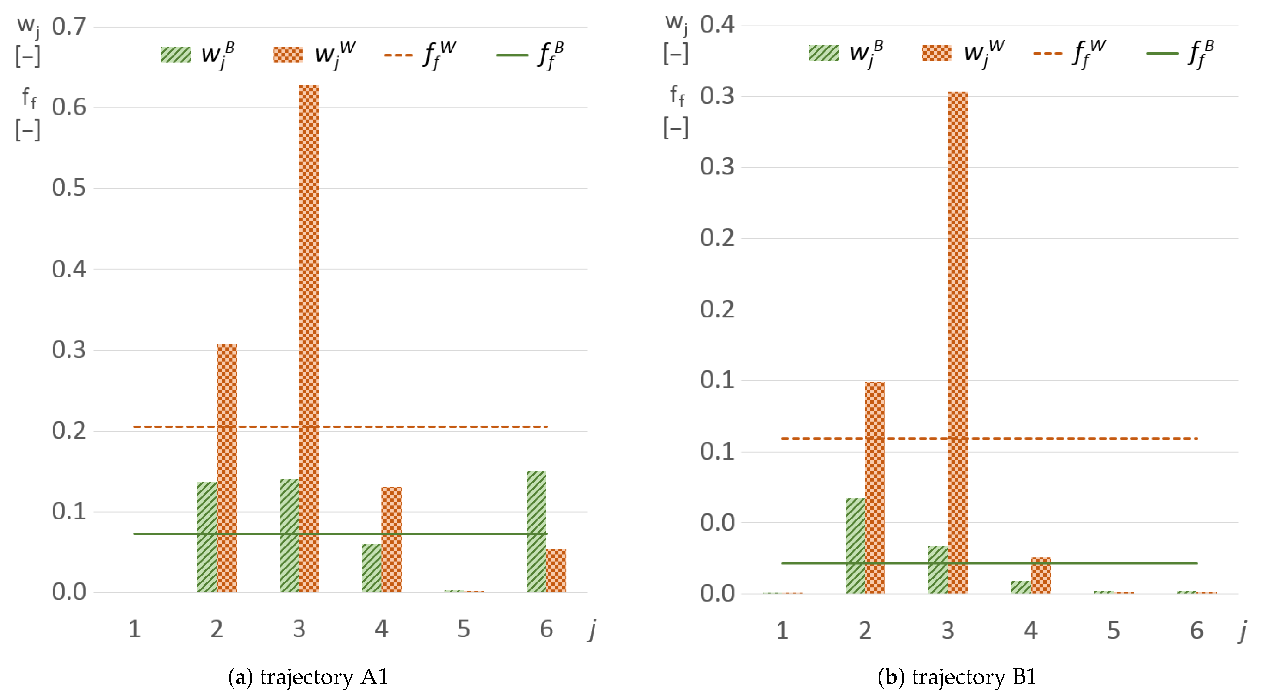
To better demonstrate the meaning of the proposed optimization criterion,
Figure 7 shows, for the two trajectories A1 and B1, the individual values of the relative joint wear factors
(
5) for the best (
) and worst (
) robot location, together with the corresponding total fitness function value
(
8). In the first example (trajectory A1), it is clear that, in the worst location, the third joint was extremely stressed and the six
values differ quite considerably. In the best location, joints 2, 3, and 6 have almost the same
values and, although the relative wear factor of the 6th joint increased, the overall
value was much lower.
A similar situation can be seen in the second image (trajectory B1). Here, the relative wear factor values in the best location are not so well balanced–the overall fitness function value was reduced considerably nonetheless because the average value
A (Equation (
6)) lowered.
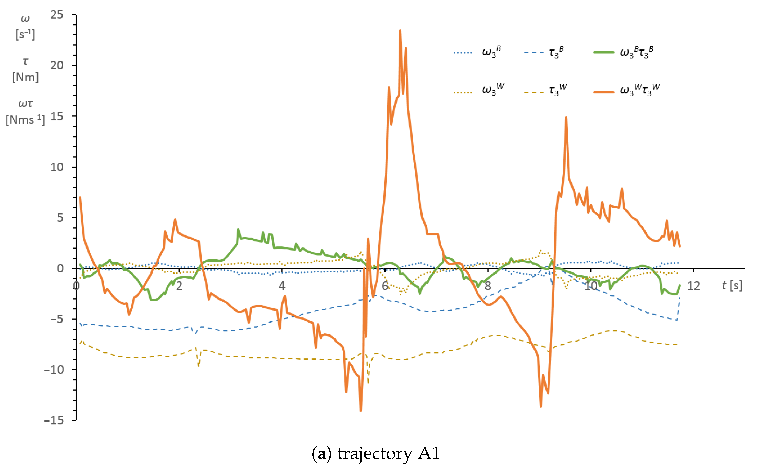
The reason for the big improvement in the third joint relative wear factor
for both these trajectories can be seen in
Figure 8—the green and red solid lines show the immediate power values for the best and worst robot location, respectively. The difference in the magnitude is evident.
4. Verification on a Real Robot
To experimentally verify the impact of the chosen fitness function on the real wear of the robot joints, it would be necessary to perform simultaneous long-term testing on multiple robots and then analyze the mechanical degradation of important components of the joint construction. This type of experiment was not feasible for us at this moment. Instead, we used experiments on a real robot to verify the accuracy of dynamical simulation in CoppeliaSim.
The real experiments were performed on the same robot as was previously used for the simulations—the Universal Robots UR3 collaborative robot. The robotic arm was mounted on a table (
Figure 2), and, instead of changing the robot base location relative to the trajectory, the trajectory was appropriately shifted in relation to the robot. There were no tools nor other equipment mounted to the output interface flange, which corresponds to the simulation model described above.
The robot controller (CB3 controller, firmware version 3.10.0) provides state messages via the RTDE (Real-Time Data Exchange) protocol based on TCP/IP communication. This protocol allows reading the actual state of the robot with a frequency of 125 Hz. The RTDE messages can be configured and include the actual and target values of kinematic parameters, such as the position, velocity, and acceleration, as well as the currents of individual joints, the overall current of the whole robot, and the target torque values—which are needed for our experiment.
The experiment was executed for the optimal (best) robot location found by the simulation, for the worst robot location, and for three other locations that were manually selected from the set of possible locations to cover various sections of the whole space. The locations are hereafter referred to as “B” (best), “W” (worst), and “1”, “2”, and “3” (the other locations). The three numbered locations are sorted from the lowest to the highest
values according to the simulation results (a lower
value indicates a better robot location). For each trajectory and robot location, the robot was programmed to go through the whole trajectory five times in a row. During this time, the integral (sum) was calculated according to (
4), and the final value was then divided by five.
All tested real robot locations are depicted in
Figure 6. Numerical values of the
values in all five locations for all ten trajectories are listed in
Table 3 and
Table 4.
Table 3 shows the results from the simulation, the values here are sorted from lowest to highest (“B”, “1”, “2”, “3”, and “W”).
Table 4 shows the values from real experiments—as can be seen, the best locations were identical; the worst locations were also mostly identical, except for trajectory D2.
Table 5 shows the ratios between the real and simulated values; ideally, these values should all be equal to 1. In general, it can be stated that the
values acquired by the real experiments were lower than the values from the simulation, and the average ratio was
with the standard deviation equal to
.
Figure 9 displays a comparison of the simulated and real values in the form of a bar graph, together with the ratio
r. In this image, it can be observed that, for the same trajectory, the ratio
r typically lowers (deteriorates) with increasing the
values. This will be further discussed in the Discussion section.
5. Discussion
The paper describes the grid approach to finding the optimal robot location, where all possible robot locations are evaluated using a simulation in CoppeliaSim, and then the location with the best (lowest) fitness function value is selected. In our case, there was an additional preprocessing step that found all valid robot locations using a simple and fast custom-made simulation system to increase the speed of the process. This step is not required, and therefore the research can be reproduced without this custom simulation system.
The grid approach can alternatively be replaced by using some optimization algorithms, for example, the Particle Swarm Optimization (PSO) [
31], which could further reduce the time needed to find the optimal solution. However, PSO would not provide the same type of comprehensive analysis of the whole space around the trajectory, and could also possibly return a local minimum instead of the global one.
The method was demonstrated and tested on ten sample trajectories and the collaborative robot UR3. As can be seen from the results in
Table 2, the percentage improvement in the fitness function between the worst and the best possible robot location ranged from 54% to 80.3%. This is mostly a theoretical improvement, as the worst-rated locations would likely be not chosen by the system integrator or workplace project architect for other reasons (they are typically on the edge of the working area of the robot or close to a singular configuration). If we instead compare the best robot location to the average
value of all possible locations, the improvement still ranges from 22% to 53.1%; therefore, it is clear that some interesting reduction in the robot joints wear can be achieved by selecting the optimal robot location instead of a “random” one.
This method can be used in practice, provided there is a dynamic model of the selected robot available for some suitable simulation system (for example, CoppeliaSim). It is necessary to properly define the whole simulation model of the workplace, including any potential obstacles, otherwise, the returned optimal robot location could be invalid due to a collision. Nonetheless, it is still important to verify that the optimal location is feasible from the point of view of energy connections and other similar restrictions that cannot be included in the simulation.
The dynamic model should include all properties and phenomena that noticeably affect the torque values in joints of the robot, as the torques are one of the main inputs for the proposed method. It is, thus, necessary to properly define and simulate also the payload in the end-effector, including any technological forces caused by the effector during, for example, cutting, milling, and spraying. The simulation system CoppeliaSim chosen in our demonstration is capable of simulating all these effects.
Experiments on a real robot UR3 verified that the simulation model in CoppeliaSim matched the reality acceptably well. The absolute values of acquired by the simulation and from the real robot differed approximately by the scale factor of 0.745 ± 0.126.
The difference between simulation and reality was caused especially by the simulation model of the UR3 robot, which is likely not absolutely perfect as far as mass properties are concerned, and also by the dynamic simulation engine, which performed some simplifications. More important is that, in the relative evaluation of individual robot locations, the real experiments led to very similar results as the simulation—as can be seen in
Table 3,
Table 4 and
Table 5. There were some distinct deviations only in one path of robot end-point movement (trajectories D1, D2). It can be, thus, stated that, to improve the robot joints wear, potentially expensive and time-consuming real-world experiments are not necessary; a simulation suffices.
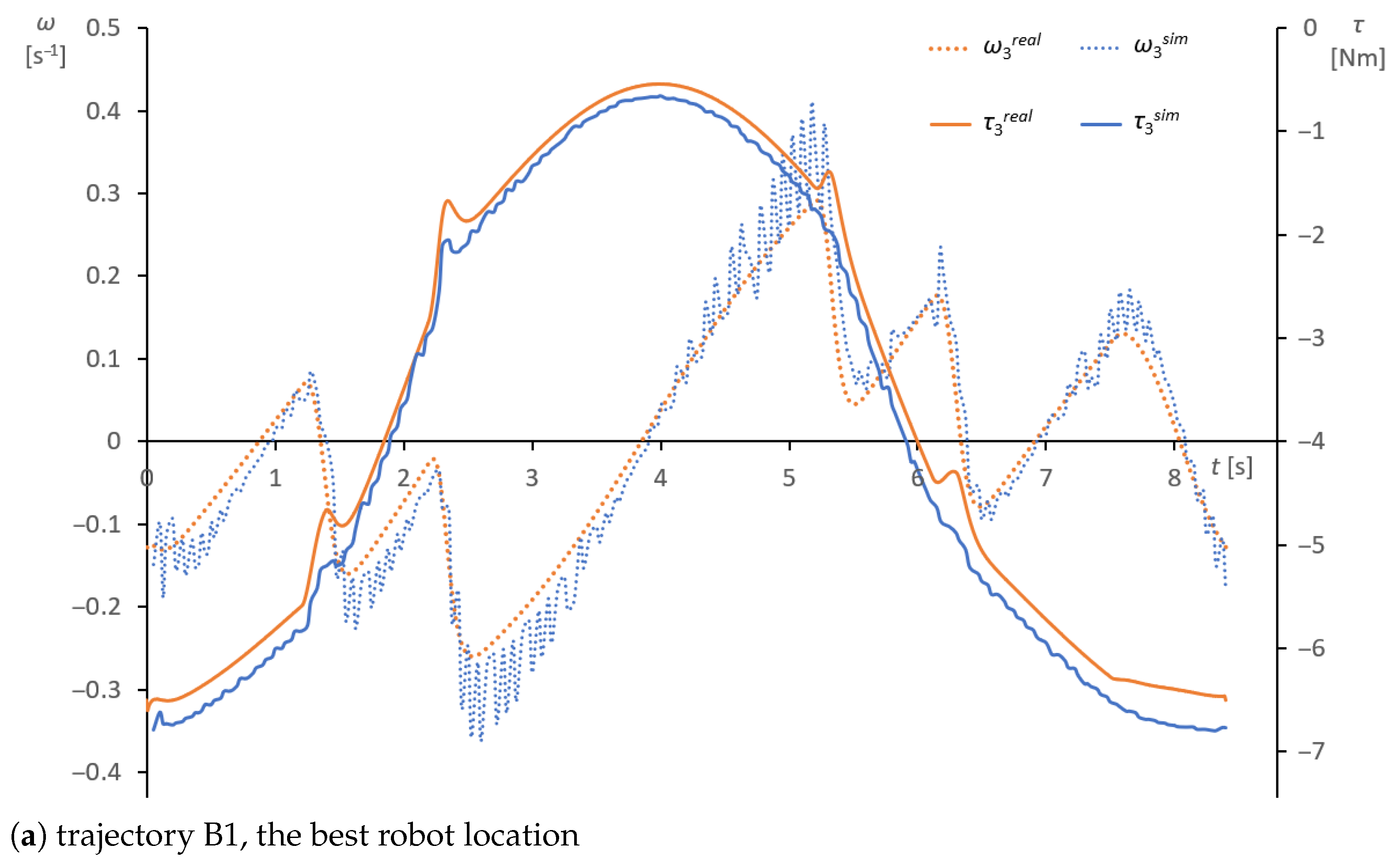
To demonstrate and analyze the source of the difference between the values from the simulation and from the real robot,
Figure 10 shows an example of the simulated torque
and velocity
values directly compared with the values from the real robot (
,
), for the third joint of the robot during the B1 trajectory. The absolute value of
was generally lower than the absolute value of
, which was likely caused by inaccurate mass parameters of the robot links in the simulation model. This is the reason why the
values from the real robot were mostly lower than the values from the simulation (see
Table 5). The noise in the
values was caused by the discrete character of the simulation.
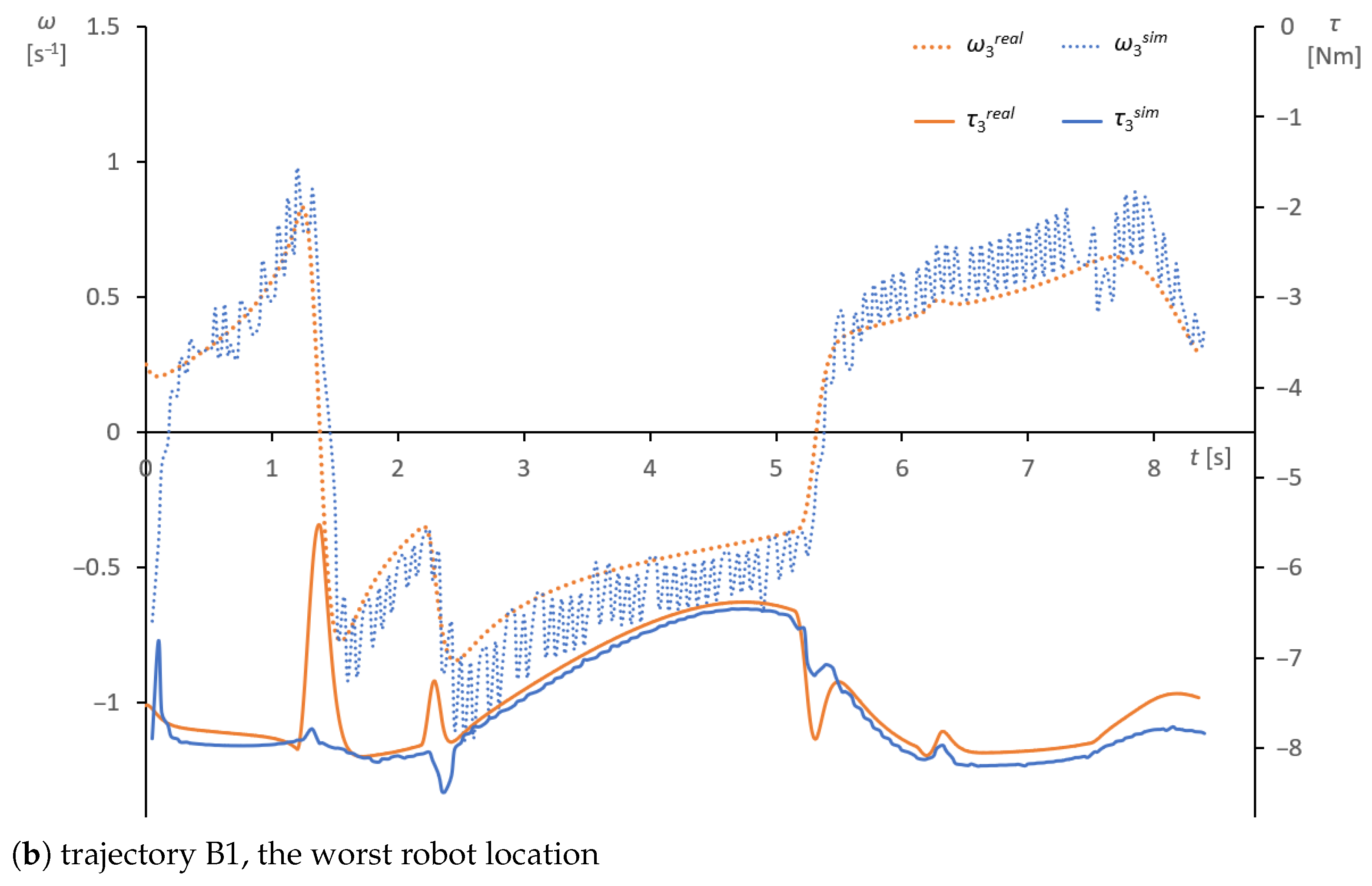
Figure 10b shows that, for the worst robot location, the
values differed significantly from
in several peaks that correspond to moments with noticeable acceleration in the movement. This is probably caused by some simplifications in the dynamics engine in the simulation system or by some advanced algorithms in the control system of the real robot. Generally, in worse robot locations (with higher
values), the robot joints must perform movements with higher acceleration, which causes this additional source of difference between the simulation and reality.
The proposed optimization process of a robotized workplace can be applied in the design phase when it is easy to make modifications to the workplace layout. Another option is to use the optimization for an existing workplace when other types of optimization are not possible (the trajectory is fixed, etc.).
6. Conclusions
The goal of this paper was to present a methodology for the optimization of a robot manipulator base position relative to the given trajectory of movement of the manipulator end-point. The optimization algorithm was based on the principle of minimization of the chosen fitness function, which comprises the arithmetic mean and standard deviation of the relative wear factors of all robot joints (
8). The goal was to balance and minimize the wear of the drive chain in the robot joints, where the wear is approximated as the amount of mechanical work done by the joint, while also taking into account the abilities of the particular joint (the maximal permissible torque and velocity).
Future work will include verification on different types of robots and with various payloads. To verify the real impact on the wear of robot joints and, thus, the reduction of the robot lifetime, a long-term experiment would have to be performed simultaneously on at least two identical robots. One robot would be placed in a location with a good (low) value and the other—reference—robots would perform the same task from locations with higher values. Afterward, the robots would have to be partially disassembled to analyze and compare the mechanical degradation of the joints.
The cases when the workplace is used alternately for several different tasks and, thus, the robot performs more than one movement trajectory could also be addressed. The trajectories could either be combined into one for the simulation, or the method could be applied to each trajectory separately and then the results would be combined, for example by interpolation using weight coefficients given by the frequency of use of the trajectories.
Although this method does not require extremely precise dynamic simulation, this aspect could also be improved by creating a more accurate dynamic model of the robot, for example using some of the dynamic parameter identification method [
32]. However, the simulation of friction and other complex phenomena will always be simplified in commonly available simulation systems.


 ,
, 


