Automatic Microscopy Analysis with Transfer Learning for Classification of Human Sperm

Abstract

Infertility is a global problem that affects many couples. Sperm analysis plays an essential role in the clinical diagnosis of human fertility. The examination of sperm morphology is an essential technique because sperm morphology is a proven indicator of biological functions. At present, the morphological classification of human sperm is conducted manually by medical experts. However, manual classification is laborious and highly dependent on the experience and capability of clinicians. To address these limitations, we propose a transfer learning method based on AlexNet to automatically classify the sperms into four different categories in terms of the World Health Organization (WHO) standards by analyzing their morphology. We adopt the feature extraction architecture of AlexNet as well as its pre-training parameters. Besides, we redesign the classification network by adding the Batch Normalization layers to improve the performance. The proposed method achieves an average accuracy of 96.0% and an average precision of 96.4% in the freely-available HuSHeM dataset, which exceeds the performance of previous algorithms. Our method shows that automatic sperm classification has great potential to replace manual sperm classification in the future.

1. Introduction

Infertility is a worldwide problem that affects more than 10% of couples, among which about 30% to 50% are found to be related to men [1]. Sperm quality is the most important criterion for measuring male reproductive ability. The quality of human sperm not only affects the probability of conception but also profoundly impacts the physical and mental health of offspring. Sperm analysis is an essential step to identify sperm quality in clinical diagnosis. Generally, analysis of sperm cells includes sperm motility detection and sperm morphology examination. Sperm morphology is a proven indicator of male fertility [2], and morphology assessment classifies the sperm in multiple categories [3,4]. Previous studies have shown that teratozoospermia (i.e., the increased concentration of abnormal sperms) is affected by various factors, such as aging and genetics [5,6]. Therefore, morphological classification of sperm is helpful to promote pathological research in human reproduction. Besides, in vitro fertilization also needs to find sperm with excellent quality quickly, which further requires the rapid and accurate classification of sperm.

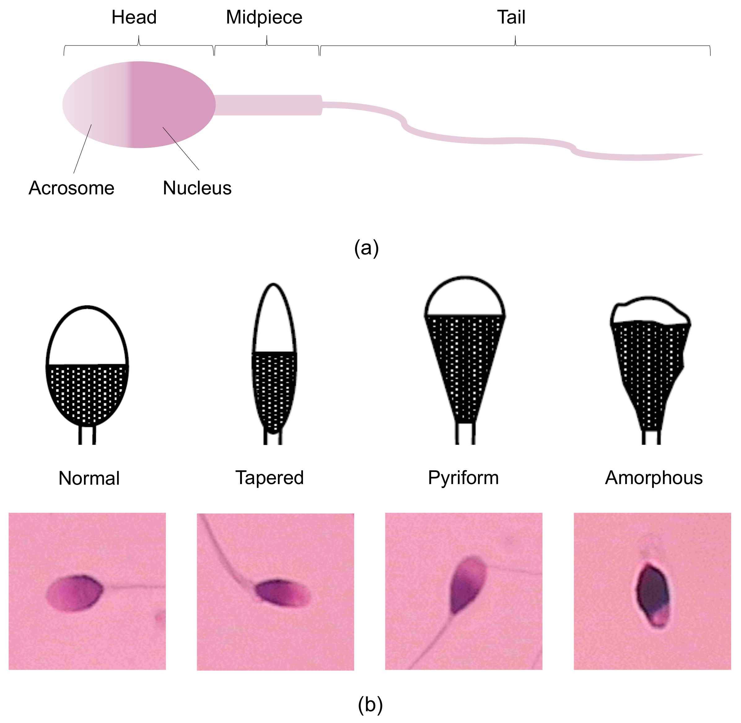
Human sperm consists of three main parts: head, midpiece and tail (Figure 1a) [7]. According to the World Health Organization, human sperm can be divided into normal sperm and abnormal sperm, and the abnormal sperm can be further classified into four sub-categories: head defects, neck and midpiece defects, tail defects, and excess residual cytoplasm [8]. Among these defects, head defects, including tapered, pyriform, no acrosome, small, amorphous, vacuolated and small acrosomal areas, have the most significant impact on sperm quality [8]. Herein, we mainly focus on the head malformations in this research. Although the Computer-Assisted Semen Analysis (CASA) system has been applied in various scenarios for semen analysis, it has not yet been able to classify human sperm morphologically [9]. In clinical applications, human sperm morphology analysis is conducted manually by experienced physicians, which is laborious, time-consuming, and highly subjective [10,11].

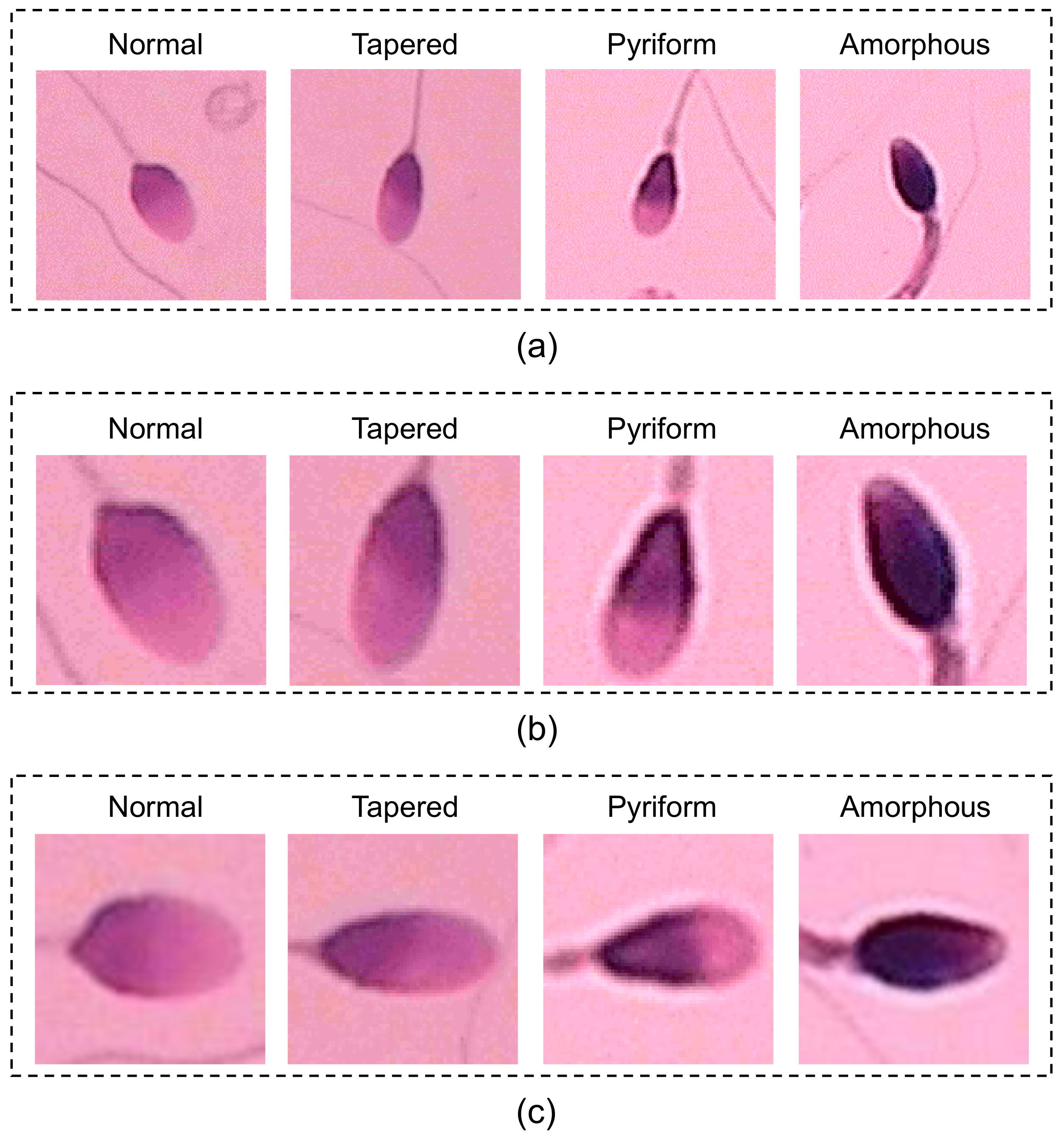
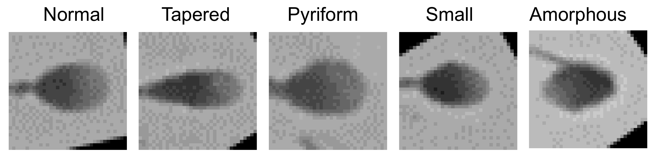
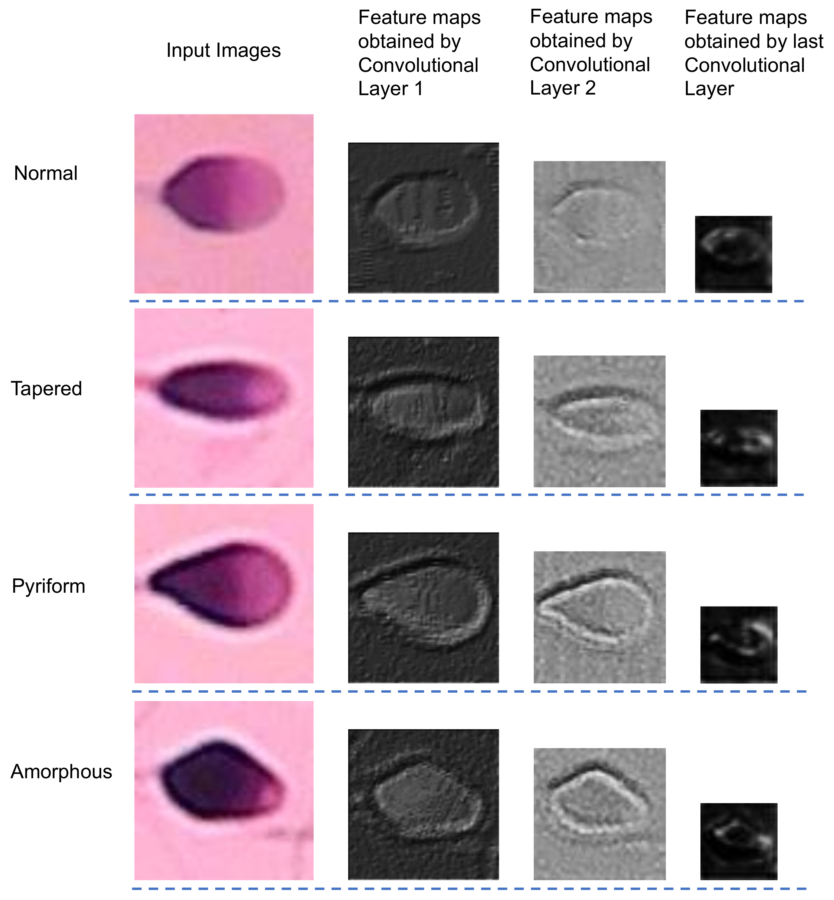
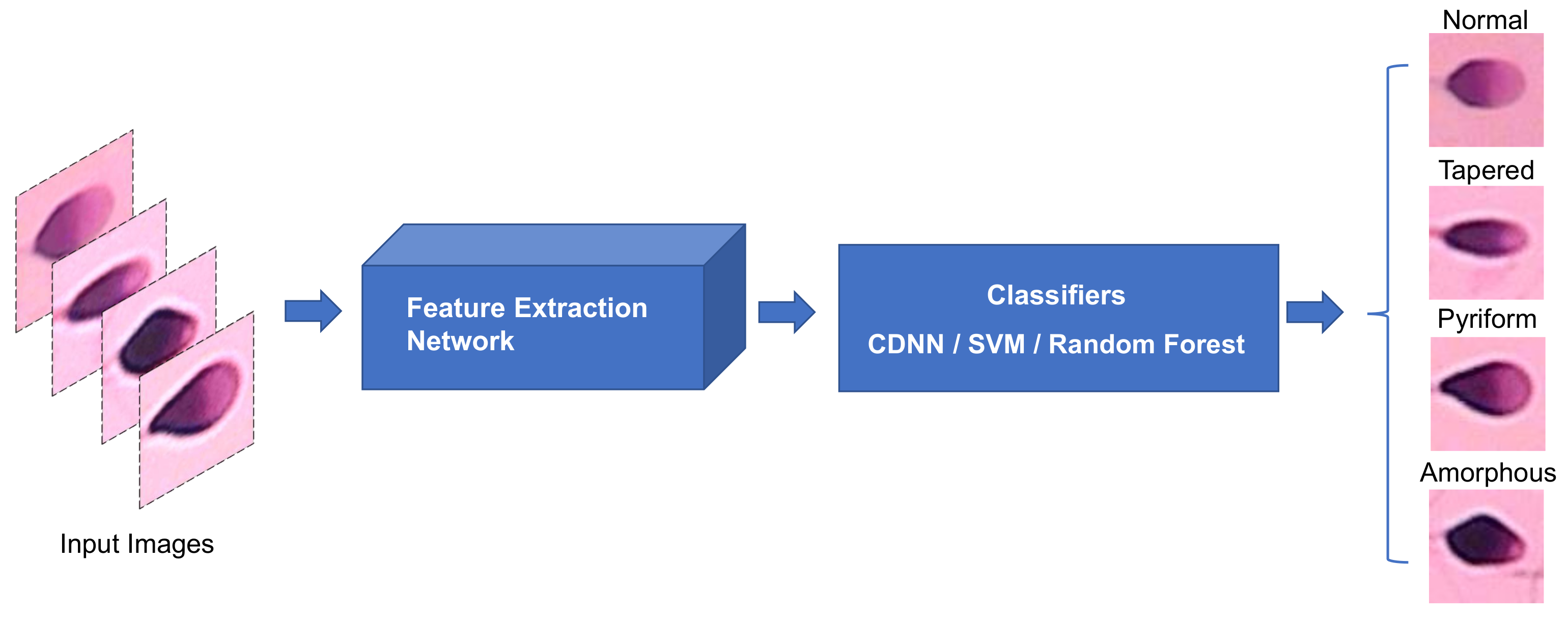
To address the limitations of manual human spermatozoon classification, researchers have recently developed various automatic sperm morphology classifiers. According to WHO criteria, the four classes of sperm heads, namely tapered, pyriform, amorphous, and normal sperm (as shown in Figure 1b), are almost indistinguishable by embryologists because they have limited differences. Therefore, the classification algorithms are mainly focused on the classification of these four categories.

The earliest algorithms for sperm head classification were based on traditional machine learning methods. In 2017, Chang et al. introduced a gold-standard tool (SCIAN-MorphoSpermGS dataset) to evaluate and compare the classification approaches for human sperm heads [12]. The SCIAN dataset consists of 1854 sperm cell images and includes five different expert-classification categories: normal, tapered, pyriform, small, and amorphous. Subsequently, they proposed a two-stage algorithm to classify sperm heads into the five aforementioned classes of the SCIAN dataset and achieved an average classification accuracy of 58% [13]. In the first stage, the amorphous sperm cells are filtered out, while the remaining four classes are also preliminarily classified. The second stage works as a verifier to verify the results of the previous stage. In another study, Shaker et al. employed an adaptive patch-based dictionary learning (APDL) approach to improve the average true positive rate to be 62% on the SCIAN dataset and achieve an average true positive rate of 92.3% on the HuSHeM dataset for automatic sperm head classification [14]. In the APDL scheme, small square patches are acquired from the sample sperm head images to train the algorithm and the patches of the test images from class-specific dictionaries are recreated to match the test data to the corresponding class.

Despite the great progress in human sperm classification tasks, these approaches require the features of sperm heads to be extracted manually and then fed into the classifier for training purposes, making it extremely difficult to classify the cells end-to-end. In the past few years, the emergence of deep learning has dramatically boosted the performance of state-of-art techniques in computer vision tasks [15,16,17,18,19,20]. In terms of automatic image classification, deep convolutional neural networks (CNNs) have demonstrated higher classification accuracy than traditional machine learning algorithms. More importantly, the CNNs are able to process raw data without extracting data features manually. In 2019, Riordon et al. applied a CNN-based method to the sperm cell classification task for the first time and achieved an average accuracy of 94.1% on the HuSHeM dataset and an average accuracy of 62% on the SCIAN dataset [21]. In their study, the original VGG16 network [22] was optimized for the sperm head classification task. Although the classification results are improved, the high complexity of the network structure requires large computational resources that are not available in typical IVF clinics.

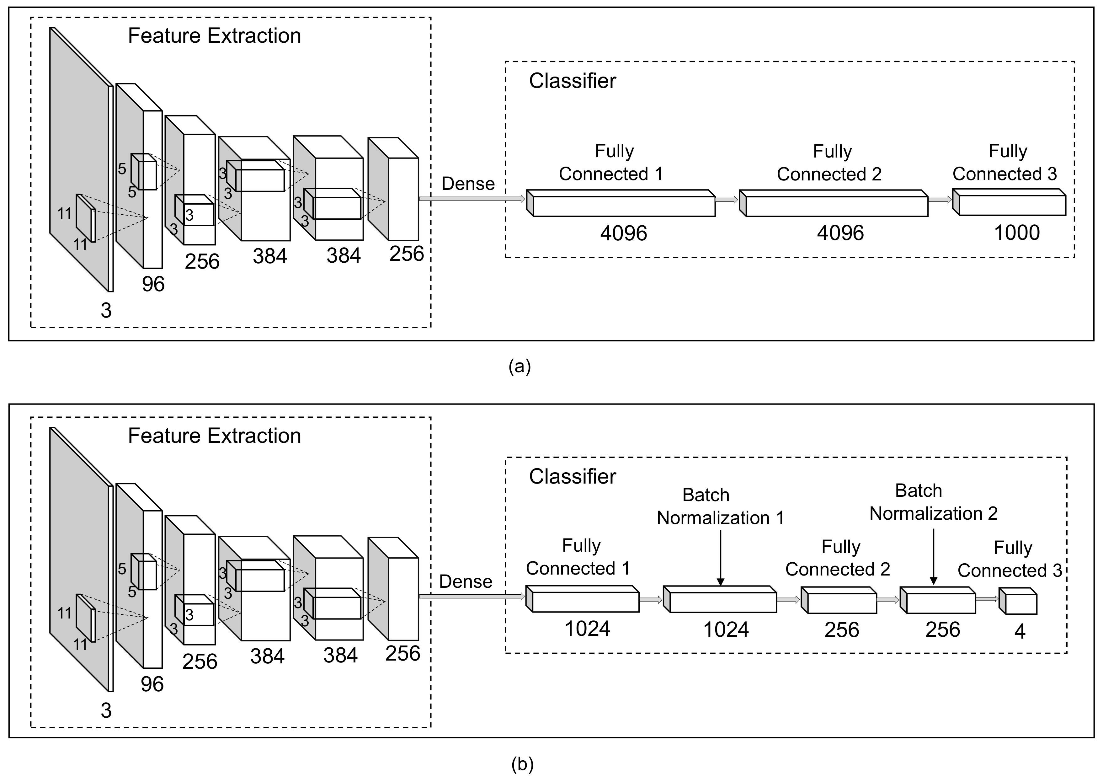
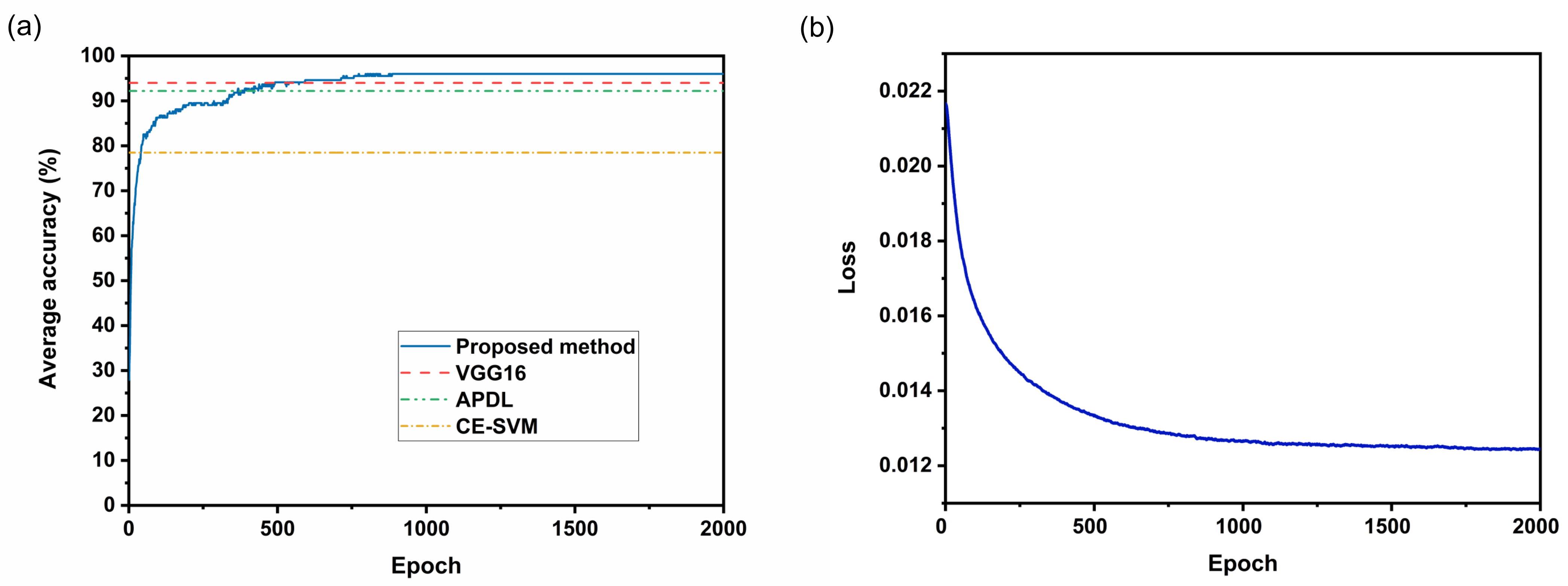
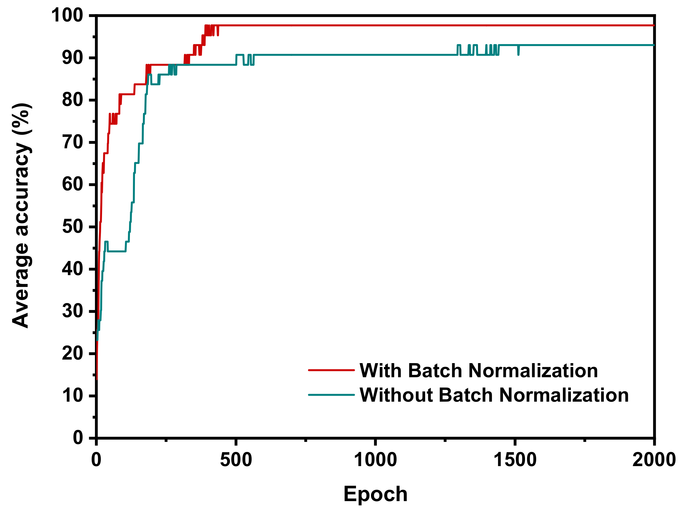
In this paper, we propose to use a different deep learning approach to classify sperm heads automatically. Instead of building the deep CNN from scratch, we modify the original AlexNet [23] by adding the Batch Normalization layers for sperm head classification for the HuSHeM dataset. Simultaneously, the pre-training parameters obtained from the training of the ImageNet dataset [24] for the feature extraction are adopted to reduce computational and time costs. The experiment results indicate our approach outperforms the state-of-the-art in terms of average classification accuracy (96.0% vs. 94.0%), average precision (96.4% vs. 94.7%), average recall (96.1% vs. 94.1%) as well as average F-score (96.0% vs. 94.1%) on the HuSHeM dataset. Moreover, compared with the VGG16-based approach presented in [21], the pre-training part our method does not require any fine tuning, and the number of parameters in the feature extraction part is less than one-sixth of those using VGG16. Accordingly, our method is relatively computer-resource-saving and has a low computational cost.

The rest of the paper is organized as follows. The model and the dataset used to test the algorithm are introduced in Section 2. Section 3 presents the experimental results, the ablation analysis of the classifier, as well as the influence of data preprocessing on the performance of the model. Finally, Section 4 concludes this work.

2. Materials and Method

2.1. Dataset Description

In this study, the HuSHeM dataset, a publicly available dataset for evaluating the sperm head classification algorithms, is used to investigate the proposed method. The samples were acquired from 25–38 years old patients at Isfahan Fertility and Infertility Center (IFIC) and then processed by the Diff-Quik method. After a series of biochemical treatments, sperm images were obtained under the microscope with a camera. More details about the HuSHeM dataset are available in [25]. According to the WHO criteria, the sperm samples in the HuSHeM dataset are classified and labeled by three specialists into four categories: normal, tapered, pyriform and amorphous (see Figure 2a). Totally 216 sperm cell images (54 normal, 53 tapered, 57 pyriform, and 52 amorphous) constitute the HuSHeM dataset and each image is in RGB format with the size of 131 × 131 pixels.

2.2. Data Preprocessing

In deep learning sector, to make the models learn the characteristics of the data better, dataset is commonly preprocessed before being feed into the algorithms [26,27]. Instead of enhancing the dataset by enlarging the number of training images, a more concise and effective data preprocessing method is adopted here. Due to the limited amount of available data in HuSHeM dataset, to make full and effective use of each sample, the sperm heads in the images were cropped and rotated to the same direction before being fed into the network. To boost the image preprocessing efficiency, a specific program based on OpenCV was developed to automatically crop and rotate the images in batches.

The flow diagram of the image preprocessing method is shown in Figure 3. The original image (Figure 3a) was first denoised and converted to monochrome image. The Sobel operator was then applied to obtain the gradient image with high horizontal gradient and low vertical gradient, as shown in Figure 3b. Subsequently a low-pass filter was employed to remove the high-frequency noise in the gradient image, and the resulting image was binarized using an adaptive thresholding algorithm. To find out the contour of the sperm head, the binary image was morphologically eroded and dilated to eliminate interference spots (Figure 3c). Then, the contour of the sperm head was processed by elliptical fitting to obtain the major and minor axis (Figure 3d). Finally, the main feature area centered on the ellipse, namely the head of the sperm (Figure 3e), was cropped. As a result, a dataset consists of images with the size of 64 × 64 pixels containing valid information of about the sperm head was obtained, as shown in Figure 2b.

In order for the algorithm to learn the characteristics of different types of sperm precisely, we also investigated the influence of the head orientations of the sperm. In the experiments, the head of the sperm was aligned to the uniform direction (i.e., pointing to the right as shown in Figure 3f. The rotated image was further cropped with the same image size (See Figure 3g). The example images of the acquired dataset are shown in Figure 2c. The performance of the algorithm on the three distinct datasets (i.e., Figure 2a–c) is compared in the Section 3.

2.3. Transfer Learning Method

Since deep CNNs have achieved unprecedented results in many complicated computer vision classification tasks, it is proper to employ a deep CNN to deal with sperm cells classification problems. Here, the original AlexNet initially proposed by Krizhevsky in [23], as shown in Figure 4a, was modified to classify the sperm into corresponding classes morphologically. The architecture of the AlexNet-based transfer learning model for sperm image classification is shown in Figure 4b.

AlexNet can be divided into two parts, the feature extraction and the classifier. The first five convolutional layers extract the features of the input image, and the remaining three fully-connected layers classify the acquired features. Three Max-pooling layers, which are used to better summarize the outputs of neighboring layers, follow the first two convolutional layers as well as the fifth convolutional layer respectively. The size of convolution kernels and the number of channels are depicted in the Figure 4a. Dropout layers are employed after the first two fully-connected layers to reduce overfitting in the classifier. In the proposed approach, the intact feature extraction part of AlexNet with pre-trained parameters on the ImageNet was adopted to be the feature extractor for capturing the spatial information of the sperm heads. Compared with the original AlexNet model, the classifier was rewritten to better suitable for the task. The nodes of the first two fully connected layers in the prediction part were redesigned. Besides, following each ReLU activation function with the fully-connected layer, a Batch Normalization was added to improve the performance of the algorithm. Although Batch Normalization was introduced primarily for accelerating the training speed of deep CNNs by reducing internal covariate shift, it also increased the accuracy of specific classification algorithms [28]. The number of neurons in the last fully-connected layer is equal to the number of sperm categories, and a softmax layer was implemented in the final fully-connected layer. The information of the hyperparameters in classifier of the proposed network is summarized in

Table 1. The hyperparameters in the classifier of the proposed network.

Hyperparameters	Value	Hyperparameters	Value
Fully Connected 1	1024	Dropout 2	0.5
Batch Normalization 1	1024	Fully Connected 3	4
Dropout 1	0.5	Learning rate	0.00001
Fully Connected 2	256	Batch size	64
Batch Normalization 2	256	Training epochs	2000

.

2.4. Implementation

To better compare with the previous methods, the 5-fold rotation estimation was employed in our approach. The dataset was randomly divided into five sub-samples, of which a single sub-sample was retained as the test data for the verification model, and the other four sub-samples formed the training set. Cross-validation was repeated five times, and each sub-sample was verified once. The final results were averaged five times to achieve the single performance estimation for the proposed model. Another benefit of the 5-fold cross-validation is that it can alleviate overfitting, which is a common problem for training small datasets like HuSHeM. The number of images in the HuSHeM dataset allocated in each fold is summarized in

Table 2. Number of images allocated to each group for the 5-fold cross-validation.

Group	Data Types	Normal	Tapered	Pyriform	Amorphous
Group 0	Train	43	42	46	42
	Test	11	11	11	10
Group 1	Train	43	42	46	42
	Test	11	11	11	10
Group 2	Train	43	43	45	42
	Test	11	10	12	10
Group 3	Train	43	43	45	41
	Test	11	10	12	11
Group 4	Train	44	42	46	41
	Test	10	11	11	11

.

As the feature extraction part of the original AlexNet and its pre-training parameters remained intact, the code for this part was programmed using the built-in algorithms of the PyTorch document. The feature interpreter and regression part of the proposed model was programmed in PyTorch (1.7.1) with Python (3.7.8). The algorithm was trained on a DELL workstation with a CPU of Intel(R) Xeon(R) Gold 6226R @2.90 GHz and an NVIDIA Quadro RTX 4000 GPU with 8GB memory using the Jupyter Notebook (6.1.5). The Adam optimizer was chosen to be the learning algorithm with a fixed learning rate of 0.00001 in the proposed model. According to the classification accuracy, the hyperparameters of the model were optimized iteratively. Finally, the best hyperparameter configuration for a specific task here is shown in Table 1.

During the training process, the parameters of the transfer learning part (i.e., feature extractor) were frozen. Only the parameters in the redesigned prediction layers were trained to accelerate the parameter optimization process and save computing resources. Figure 5a shows how the test accuracy changes with training steps. The test accuracy grows rapidly in the initial part of the training and then rises gradually. A corresponding change is also observed in the loss, as shown in Figure 5b. The loss drops sharply at the beginning and then decreases progressively. However, the test accuracy does not necessarily increase with the training steps, possibly due to overfitting problems. Sometimes, the best test accuracy even appeared in the first half of training. For example, the test accuracy reaches the maximum when the number of training steps is around 900, although the total number of training steps is set to 2000. During the validation process, the test set was enlarged by 64 times to reduce the calculation error caused by the limited test images.

3. Results and Discussion

This section may be divided by subheadings. It should provide a concise and precise description of the experimental results, their interpretation as well as the experimental conclusions that can be drawn.

3.1. Evaluation of Performance

The morphological classification of sperm head is a multi-classification task, so related metrics need to be defined in advance to evaluate the model better. Similar to the previous study in [29], for each class C${}_i$ (i is the index of corresponding class number), the evaluation metrics are given as TP${}_i$, FP${}_i$, FN${}_i$ and TN${}_i$, which denote the number of the true positive, false positive, false negative, and true negative, respectively. Additionally, the macro metrics (i.e. the average of metric of each class) is obtained to evaluate the algorithm.

The average accuracy can be expressed as:

$$\begin{array}{c}\hfill AverageAccuracy=\frac{{\sum }_{i=1}^l\frac{T{P}_i+T{N}_i}{T{P}_i+F{N}_i+F{P}_i+T{N}_i}}{l}\end{array}$$

(1)

where l is the number of the classes, the same below.

The average precision can be defined as:

$$AveragePrecision=\frac{{\sum }_{i=1}^l\frac{T{P}_i}{T{P}_i+F{P}_i}}{l}$$

(2)

The average recall can be expressed as:

$$AverageRecall=\frac{{\sum }_{i=1}^l\frac{T{P}_i}{T{P}_i+F{N}_i}}{l}$$

(3)

The average F-score can be defined as:

$$AverageF-score=\frac{{\sum }_{i=1}^{l}2\times \frac{{Precision}_i\times {Recall}_i}{{Precision}_i+{Recall}_i}}{l}$$

(4)

where Precision${}_i$ and Recall${}_i$ are the precision and recall of the i class respectively. Their expressions are shown in Equations (5) and (6).

$${Precision}_i=\frac{T{P}_i}{T{P}_i+F{P}_i}$$

(5)

$${Recall}_i=\frac{T{P}_i}{T{P}_i+F{N}_i}$$

(6)

As summarized in

Table 3. Comparison of the proposed method with the state-of-the-art algorithms.

Methods	Accuracy	Precision	Recall	F-Score
CE-SVM [13]	78.5%	80.5%	78.5%	78.9%
APDL [14]	92.2%	93.5%	92.3%	92.9%
VGG16 [21]	94.0%	94.7%	94.1%	94.1%
The proposed method	96.0%	96.4%	96.1%	96.0%

, the accuracy, precision, recall, and F-Score of the proposed approach are calculated and compared with other state-of-the-art algorithms. The values shown in the table are the average of the 5 groups. It can be seen from Table 3, the transfer learning method based on AlexNet surpasses the previous methods in terms of all four metrics (i.e., average accuracy, precision, recall, and F-Score).

In order to further investigate the performance of the proposed model in each category and the mutual influence between different categories, the confusion matrix was summarized and shown in

Table 4. The confusion matrix of the prediction in the test dataset. The percentage values of correct and incorrect prediction in the table are the average of the five groups. The values in bold represent the prediction precision of each category, and the average of them is the average precision.

		Actual
		Normal	Tapered	Pyriform	Amorphous
Prediction	Normal	99.0%	0.0%	1.7%	0.3%
	Tapered	0.5%	95.3%	3.2%	1.4%
	Pyriform	0.5%	4.4%	94.1%	1.1%
	Amorphous	0.0%	0.3%	1.0%	97.2%

. Normal sperm has the highest prediction precision (99%), while the average accuracy of tapered and pyriform sperm is relatively low (95.3% and 94.1%, respectively). The increased accuracy in the normal group is mainly attributed to the fact that the contours of normal sperm are uniform and easy to be distinguished from other species. The shape of some tapered sperms and pyriform sperms are very similar, which is likely to confuse the classifier, causing the network to misrecognize each other. The testing results also show that up to 4.4% of tapered sperm are predicted to be pyriform, while 3.2% of pyriform sperm are recognized as tapered. With the irregular profile, the amorphous sperms are also primarily differentiated from other classes. However, the large variations of amorphous sperm shape also increase the difficulty of regression in the algorithm and affect the final prediction of this category. As a result, the correctly predicted rate of amorphous is 97.2%, slightly lower than normal sperm.

The proposed approach was also evaluated on SCIAN dataset. There are five different categories of sperm head images in this dataset (100 normal, 228 papered, 76 pyriform, 72 small and 656 amorphous) and each image is with the size of 35 × 35 pixels, as shown in Figure 6. In this dataset, the samples were labeled by three experts in the minority subordinate to the majority. In other words, only images with at least 2-out-of-3 expert agreement were kept. Since there were five distinct groups of sperms in the input data, the output of the network was modified to five corresponding categories (i.e., redesign the number of neurons in the Fully Connected 3 layer to five). Because the sperm heads in the images were aligned and cropped, they could be directly fed into the model without pre-processing. The results of the 5-fold cross-validation experiment show that the average accuracy of our model on the SCIAN dataset is 62%, which is comparable to the performance of state-of-the-art methods (58% for CES-VM [13], 62% VGG16 [21]). In the experiments, we notice that, when the size of the input image is small (e.g., less than 64 × 64 pixels in the SCIAN dataset), the feature maps after multiple pooling will become smaller than that of the convolution kernel. As a result, no effective feature maps can be extracted. Therefore, the images in the SCIAN dataset need to be expanded in pixel size before feature extraction can be performed. However, the expansion of the image would inevitably cause image distortion and affect the performance of the model. In clinical applications, high resolution images can be used to achieve the optimal performance of the proposed method.

3.2. Ablation Analysis

For the human sperm morphology classification of the HuSHeM dataset, Dropout layers, and Batch Normalization layers (see Figure 4b) were employed to help the model classify the cells with higher accuracy. To investigate the influence of different components in the proposed method on the classification results, an ablation experiment was conducted. The values of the metrics obtained from the ablation experiment are shown in

Table 5. Performance of the algorithms with different configurations. Batch Normalization+Dropout: both Batch Normalization and Dropout were added to the network. Dropout: only Dropout was added to the network. Batch Normalization: only Batch Normalization was added to the network. None: network with neither Batch Normalization nor Dropout.

Configurations	BN + Dropout	Dropout	BN	None
Accuracy	96.0%	93.8%	95.7%	93.8%
Precision	96.4%	94.3%	96.1%	94.2%
Recall	96.1%	93.7%	95.7%	93.7%
F-score	96.0%	93.7%	95.6%	93.7%

. When only the Dropout layers are applied in the algorithm, the performance of the model hardly improved. This indicates that the reduced prediction accuracy of the algorithm is because the model could not learn and summarize the general characteristics of the training dataset well due to the relatively concise architecture of the method. Hence, the Batch Normalization layers were added to help the model better regress the generalized features of the input training images. With the Batch Normalization layers, the classification metrics grew by about 2% (the average accuracy, precision, recall, and F-score increased from 93.8% to 95.7%, from 94.2% to 96.1%, from 93.7% to 95.7%, from 93.7% to 95.6%, respectively). The Batch Normalization layer relieves the internal covariate shift phenomenon that refers to the change in the distribution of activations caused by the varied network parameters in the learning process. Therefore, the classifier with Batch Normalization layers could better capture the characteristics of the input data and improve the regression of the classification. On the basis of the upgraded learning capacity with Batch Normalization layers, the Dropout layer could further improved the classification performance slightly (the average accuracy, precision, recall, and F-score went up to 96.0%, 96.4%, 96.1%, and 96.0%, respectively). Finally, both Dropout layers and Batch Normalization layers were added to modify the AlexNet with transfer learning.

In addition to improving the classification accuracy, the Batch Normalization layer can also speed up the training process. In experiments, two training processes with and without Batch Normalization are compared and the training curves are plotted in Figure 7. The accuracy of the network with Batch Normalization reaches its maximum value at around 400th epochs, which is faster than that of the network without Batch Normalization (at around 1400th epochs). The results further indicate that the Batch Normalization layers can upgrade the learning ability of the classification model.

3.3. Data Preprocessing Analysis

The model with both Batch Normalization layers and dropout layers was used to evaluate the impact of data preprocessing on the learning effect of the proposed algorithm. As shown in

Table 6. Performance of the algorithms on the original HuSHeM dataset and processed datasets.

Datasets	Original	Cropped	Cropped and Aligned
Accuracy	79.4%	83.4%	96.0%
Precision	80.1%	84.9%	96.4%
Recall	79.2%	83.2%	96.1%
F-score	79.3%	83.2%	96.0%

, the evaluation indicators of the model gradually increase with data preprocessing. The average accuracy grows from 79.4% to 83.4% when the training images were cropped to a smaller size. The same trend is also observed in terms of average precision, average recall, and average F-score, increasing from 79.2% to 83.2%, from 80.1% to 84.9%, from 79.3% to 83.2%, respectively. This is because the cropped images contain only the most valid information of the sperm head with minimal disturbance from other sperms or debris. The concise information in the cropped image is helpful for the program to capture the effective features of the objects.

In most cases, the head contours of different sperm are not distinct enough, especially between the tapered and pyriform categories. Therefore, further preprocessing is needed to improve the performance of the classifier. In this study, the cropped images were rotated to orient the sperm head to the uniform direction. When the sperm heads were aligned to the same direction, the average accuracy, average precision, average recall and average F-score are greatly improved to 96.0%, 96.1%, 96.4%, and 96.0%. The significant improvement of the rotation processing is mainly attributed to the fact that the algorithm did not need to waste computation to estimate and differentiate the position and direction of the sperm. Therefore, the deep learning network can focus on the analysis of the head morphology without dealing with the spatial and orientation disturbance.

3.4. Feature Extraction Analysis

Explaining how artificial intelligence networks make decisions is a long-standing problem, but it is very meaningful, especially in the medical field, to make artificial intelligence systems trustworthy and transparent [30]. Here we try to explain the basis of the network’s decision-making by visualizing the feature maps. The feature maps extracted from the first convolutional layer, the second convolutional layer and the last convolutional layer are shown in Figure 8. It can be seen from the feature maps that the feature extraction part mainly extracts the edge information of the sperm heads, which is the most important feature to classify sperms morphologically. With the further extraction of features and multiple down-sampling, unimportant feature information is gradually ignored, while the contour information of the sperm head becomes increasingly significant. Accordingly, the pixels on the contour are more and more distinguished from the pixels in other places. This reveals that the extracted features are helpful for the classifier to distinguish between different sperms.

To further evaluate the performance of feature extraction, the feature vectors extracted by the feature extraction part of the proposed architecture were fed to the enhanced k-nearest neighbors (k-NN) [31], Support Vector Machine (SVM) [32], and Random Forest [33] classifiers for sperm morphological classification, as shown in Figure 9.

In the proposed framework, an input image with the size of 64 × 64 pixels produces a feature map with the size of 16 × 16 pixels after feature extraction. The feature map is subsequently flattened into a 1 × 256 vector and fed into different classifiers. An enhanced k-NN algorithm named Centroid Displacement-Based k-Nearest Neighbors algorithm (CDNN) [31] is employed to classify sperms according to the input feature data. Different from the k-NN algorithm [34], the CDNN algorithm adopts a more reasonable classification decision criterion. In the CDNN algorithm, the obtained k nearest neighbors to the test sample are classified into separated groups according to their labels, and then the test sample is assigned to the group with the smallest centroid displacement when the test instance is inserted into that group. Here, the k value in the CDNN algorithm was set to be ten, namely ten nearest neighbors to the test instance were returned. For SVM, an off-the-shelf SVM classifier based on one-versus-one strategy was used to perform the classification task. In this task, radial basis function was selected as the kernel in the SVM classifier. A built-in Random Forest classifier in the scikit-learn was also used to evaluate the performance of the feature extraction part of the proposed approach. In the Random Forest classifier, ten estimators were adopted to perform the task.

The same data splitting was used in all the classifiers. The performance of these classifiers on sperm morphological classification task is shown in

Table 7. The performance of different classifiers in the sperm classification task of the HuSHeM dataset.

Classifiers	CDNN	SVM	Random Forest	Proposed Method
Accuracy	92.8%	92.3%	93.9%	96.0%

. It is worth pointing out that the experiment results are achieved to confirm the effectiveness of feature extraction of our approach, so the parameters of these classifiers are not fine-tuned and optimized. It can be seen from the classification accuracy that although the performance of other classifiers is slightly worse than the proposed method, they also exceed 92%, which confirms the effectiveness of feature extraction.

Overall, both the feature maps and experiment results of different classifiers confirm the effectiveness of feature extraction of the proposed method. And the visualization of the feature maps aslo provides insight into what the black box neural network method is.

4. Conclusions

In this research, a deep Convolutional Neural Network using AlexNet structure was modified by adding Batch Normalization layers to classify sperm automatically. The proposed approach was trained and tested on the HuSHeM dataset, a publicly available sperm dataset that contains four distinct categories. Cross-validation was conducted in the experiment to evaluate the performance. The experiment results show that our method outperforms the state-of-the-art algorithms in the given metrics: classification accuracy (96.0% vs. 94.0%), average precision (96.4% vs. 94.7%), average recall (96.1% vs. 94.1%) and average F-score (96.0% vs. 94.1%).

Compared with the method using VGG structure, the proposed method applies the pre-training parameters without fine turning, which could accelerate the training process and save computing resources.Although the more advanced deep learning architectures usually achieve better performance when facing with complex scenarios (such as the ImageNet dataset), a concise network architecture might perform better if the dataset is relatively small and the feature information is not very diverse. The comparison results confirm the simple network structure is able to extract the feature effectively without overfitting. It is also worth mentioning that Batch Normalization in the proposed method can not only accelerate the learning of the network, but also improve the final sperm classification results on the HuSHeM dataset. In addition, data preprocessing can improve algorithm performance by improving data quality. In a nutshell, this research applies the transfer learning technique and presents a new deep learning model for sperm classification. The improved classification performance with reduced computational burden enables to fully automate the semen analysis in IVF applications.

References

1. Maduro, M.R.; Lamb, D.J. Understanding new genetics of male infertility. J. Urol. 2002, 168, 2197–2205. [Google Scholar] [CrossRef]
2. Enginsu, M.; Dumoulin, J.; Pieters, M.; Bras, M.; Evers, J.; Geraedts, J. Evaluation of human sperm morphology using strict criteria after Diff-Quik staining: Correlation of morphology with fertilization in vitro. Hum. Reprod. 1991, 6, 854–858. [Google Scholar] [CrossRef]
3. Auger, J. Assessing human sperm morphology: Top models, underdogs or biometrics? Asian J. Androl. 2010, 12, 36. [Google Scholar] [CrossRef] [PubMed] [Green Version]
4. Menkveld, R. Sperm morphology assessment using strict (tygerberg) criteria. In Spermatogenesis; Springer: Berlin/Heidelberg, Germany, 2013; pp. 39–50. [Google Scholar]
5. Kidd, S.A.; Eskenazi, B.; Wyrobek, A.J. Effects of male age on semen quality and fertility: A review of the literature. Fertil. Steril. 2001, 75, 237–248. [Google Scholar] [CrossRef]
6. De Braekeleer, M.; Nguyen, M.H.; Morel, F.; Perrin, A. Genetic aspects of monomorphic teratozoospermia: A review. J. Assist. Reprod. Genet. 2015, 32, 615–623. [Google Scholar] [CrossRef] [PubMed] [Green Version]
7. Shaker, F.; Monadjemi, S.A.; Naghsh-Nilchi, A.R. Automatic detection and segmentation of sperm head, acrosome and nucleus in microscopic images of human semen smears. Comput. Methods Programs Biomed. 2016, 132, 11–20. [Google Scholar] [CrossRef]
8. World Health Organization. WHO Laboratory Manual for the Examination and Processing of Human Semen; WHO: Geneva, Switzerland, 2010. [Google Scholar]
9. Amann, R.P.; Waberski, D. Computer-assisted sperm analysis (CASA): Capabilities and potential developments. Theriogenology 2014, 81, 5–17. [Google Scholar] [CrossRef]
10. Brazil, C. Practical semen analysis: From A to Z. Asian J. Androl. 2010, 12, 14. [Google Scholar] [CrossRef] [Green Version]
11. Freund, M. Standards for the rating of human sperm morphology. A cooperative study. Int. J. Fertil. 1966, 11, 97–180. [Google Scholar]
12. Chang, V.; Garcia, A.; Hitschfeld, N.; Härtel, S. Gold-standard for computer-assisted morphological sperm analysis. Comput. Biol. Med. 2017, 83, 143–150. [Google Scholar] [CrossRef]
13. Chang, V.; Heutte, L.; Petitjean, C.; Härtel, S.; Hitschfeld, N. Automatic classification of human sperm head morphology. Comput. Biol. Med. 2017, 84, 205–216. [Google Scholar] [CrossRef] [PubMed]
14. Shaker, F.; Monadjemi, S.A.; Alirezaie, J.; Naghsh-Nilchi, A.R. A dictionary learning approach for human sperm heads classification. Comput. Biol. Med. 2017, 91, 181–190. [Google Scholar] [CrossRef] [PubMed]
15. LeCun, Y.; Bengio, Y.; Hinton, G. Deep learning. Nature 2015, 521, 436–444. [Google Scholar] [CrossRef] [PubMed]
16. Huang, G.; Liu, Z.; Van Der Maaten, L.; Weinberger, K.Q. Densely connected convolutional networks. In Proceedings of the IEEE Conference on Computer Vision and Pattern Recognition 2017, Honolulu, HI, USA, 21–26 July 2017; pp. 4700–4708. [Google Scholar]
17. Ronneberger, O.; Fischer, P.; Brox, T. U-net: Convolutional networks for biomedical image segmentation. In International Conference on Medical Image Computing and Computer-Assisted Intervention; Springer: Berlin/Heidelberg, Germany, 2015; pp. 234–241. [Google Scholar]
18. Ren, S.; He, K.; Girshick, R.; Sun, J. Faster R-CNN: Towards real-time object detection with region proposal networks. IEEE Trans. Pattern Anal. Mach. Intell. 2016, 39, 1137–1149. [Google Scholar] [CrossRef] [Green Version]
19. Wang, X.; Han, S.; Chen, Y.; Gao, D.; Vasconcelos, N. Volumetric attention for 3D medical image segmentation and detection. In International Conference on Medical Image Computing and Computer-Assisted Intervention; Springer: Berlin/Heidelberg, Germany, 2019; pp. 175–184. [Google Scholar]
20. Liu, X.; Yin, J.; Liu, J.; Ding, P.; Liu, J.; Liub, H. TrajectoryCNN: A new spatio-temporal feature learning network for human motion prediction. IEEE Trans. Circuits Syst. Video Technol. 2020, 31, 2133–2146. [Google Scholar] [CrossRef]
21. Riordon, J.; McCallum, C.; Sinton, D. Deep learning for the classification of human sperm. Comput. Biol. Med. 2019, 111, 103342. [Google Scholar] [CrossRef] [PubMed]
22. Simonyan, K.; Zisserman, A. Very deep convolutional networks for large-scale image recognition. arXiv 2014, arXiv:1409.1556. [Google Scholar]
23. Krizhevsky, A.; Sutskever, I.; Hinton, G.E. ImageNet classification with deep convolutional neural networks. Commun. ACM 2017, 60, 84–90. [Google Scholar] [CrossRef]
24. Deng, J.; Dong, W.; Socher, R.; Li, L.J.; Li, K.; Fei-Fei, L. Imagenet: A large-scale hierarchical image database. In Proceedings of the 2009 IEEE Conference on Computer Vision and Pattern Recognition, Miami, FL, USA, 20–25 June 2009; pp. 248–255. [Google Scholar]
25. Shaker, F. Human Sperm Head Morphology Dataset (HuSHeM). Available online: https://data.mendeley.com/datasets/tt3yj2pf38/1 (accessed on 24 June 2017).
26. Shorten, C.; Khoshgoftaar, T.M. A survey on image data augmentation for deep learning. J. Big Data 2019, 6, 1–48. [Google Scholar] [CrossRef]
27. Wang, J.; Perez, L. The effectiveness of data augmentation in image classification using deep learning. arXiv 2017, arXiv:1712.04621. [Google Scholar]
28. Ioffe, S.; Szegedy, C. Batch normalization: Accelerating deep network training by reducing internal covariate shift. In Proceedings of the International Conference on Machine Learning (PMLR 2015), Lille, France, 7–9 July 2015; pp. 448–456. [Google Scholar]
29. Sokolova, M.; Lapalme, G. A systematic analysis of performance measures for classification tasks. Inf. Process. Manag. 2009, 45, 427–437. [Google Scholar] [CrossRef]
30. Holzinger, A.; Langs, G.; Denk, H.; Zatloukal, K.; Müller, H. Causability and explainability of artificial intelligence in medicine. Wiley Interdiscip. Rev. Data Min. Knowl. Discov. 2019, 9, e1312. [Google Scholar] [CrossRef] [PubMed] [Green Version]
31. Nguyen, B.P.; Tay, W.L.; Chui, C.K. Robust biometric recognition from palm depth images for gloved hands. IEEE Trans. Hum. Mach. Syst. 2015, 45, 799–804. [Google Scholar] [CrossRef]
32. Chang, C.C.; Lin, C.J. LIBSVM: A library for support vector machines. ACM Trans. Intell. Syst. Technol. (TIST) 2011, 2, 1–27. [Google Scholar] [CrossRef]
33. Breiman, L. Bagging predictors. Mach. Learn. 1996, 24, 123–140. [Google Scholar] [CrossRef] [Green Version]
34. Fix, E.; Hodges, J. Discriminatory Analysis, Nonparametric Discrimination: Consistency Properties USAF School of Aviation Medicine; Technical Report 4; USAF School of Aviation Medicine: Randolph Field, TX, USA, 1951. [Google Scholar]
Figure 1. Sperm morphology: (a) Different parts of a sperm. (b) Four different categories of sperm in the HuSHeM dataset compared with the WHO schematic drawings.
Applsci 11 05369 g001
Figure 2. The processing of the dataset. (a) The original HuSHeM dataset. (b) The dataset composed of cropped images. (c) The dataset composed of aligned and cropped images.
Applsci 11 05369 g002
Figure 3. The visualization of image preprocessing. (a) The original image. (b) The gradient image. (c) The binary image after being morphologically eroded and dilated. (d) Ellipse fitting to the sperm head. (e) The cropped image. (f) The alighed image. (g) The aligned and cropped image.
Applsci 11 05369 g003
Figure 4. The architecture of the deep learning network. (a) The original AlexNet. (b) The optimized AlexNet networks for sperm classification.
Applsci 11 05369 g004
Figure 5. The training process of the AlexNet-based transfer learning method. The average accuracy of CE-SVM [13], APDL [14] and VGG16-based method [21] are also present for comparison. (a) The average accuracy varies with epochs. (b) The training changes loss with epochs.
Applsci 11 05369 g005
Figure 6. The SCIAN dataset [12].
Applsci 11 05369 g006
Figure 7. Changes in the training curves of networks in the same dataset with or without Batch Normalization.
Applsci 11 05369 g007
Figure 8. The visualization of feature maps.
Applsci 11 05369 g008
Figure 9. Different classifiers perform sperm morphological classification based on the features extracted by the same feature extraction network used in the proposed method.
Applsci 11 05369 g009