Semi-Analytical Method for Computing Effective Thermoelastic Properties in Fiber-Reinforced Composite Materials

Abstract

Effective elastic and thermal properties for isotropic or transversely isotropic thermoelastic fibrous composite materials are obtained. Fibers are distributed with the same periodicity along the two perpendicular directions to the fiber orientation. The periodic cell of the composite has a square or hexagonal distribution. Perfect contact between the fiber and the matrix is presented. The effective properties are calculated using a semi-analytical method. The semi-analytical method consists of obtaining the differential equations that describe the local problems using the Asymptotic Homogenization Method. Then, these equations are solved using the Finite Element Method. Effective elastic coefficient ($\overline{\mathit{C}}$), effective thermal expansion coefficient ($\overline{\mathit{\alpha }}$) and the effective thermal conductivity ($\overline{\mathit{\kappa }}$) are obtained. The numerical results are compared with the semi-analytical solution and with results reported by other authors. Additionally, the effective properties for a fiber with an elliptical cross section are calculated. Distributions of the fiber’s cross section with different orientations are also studied. A MATLAB program for computing the effective coefficients is presented.

1. Introduction

A composite material is a combination of two or more materials with different physical and (or) chemical properties. A composite material usually has characteristics that do not correspond to those of its isolated components [1]. Thermoelastic composites constitute an important class of materials with a wide variety of applications ranging from aerospace structures and electronic printed circuit boards to recreational and commercial equipment. Some of the most important and useful properties of these composites are lightweight, high strength and stiffness, excellent frictional properties, good resistance to fatigue and retention of these properties at high temperatures [2]. The effective thermo-mechanical properties of the composite depend on properties of the constituents and the fiber volume fraction.

Previous knowledge of physical properties of composite materials is one of the problems that science faces. Success in practical applications of composites largely depends on the possibility to predict their properties and behavior through the development of appropriate models. Numerous studies and investigations have been carried out to obtain the properties of composite materials [3,4,5,6]. The prediction of global homogenized properties based on knowledge of the composite constituents provides a useful tool for the design of composite materials. Homogenization methods have proven to be powerful techniques for the study of heterogeneous media. Among the homogenization methods, one of the most used methods is the Asymptotic Homogenization Method (AHM). The AHM can provide overall material constants which describe the global behavior of the composite structure. First, the periodic cell is identified; then, by means of the AHM [7,8,9,10,11,12], the original constitutive relations with rapidly oscillating material coefficients are transformed in two sets of mathematical problems. The first set has new physical relations over the periodic cell with constant coefficients which represent the properties of an equivalent homogeneous medium and they are called the effective coefficients of the composite under study. The second set allows the calculation of some functions which are solutions of the so-called local problems. The local problems are solved over the periodic cell. A state-of-the-art review where the AHM is applied to composites is provided in ref. [13]. A variety of existing homogenization methods are presented with their advantages and disadvantages.

Previous research has been performed for the estimation of the effective properties in composite materials. The elastic properties of carbon nanotube/polymer composites are computed in ref. [14]. A combination of the Finite Element Method (FEM) and the Strain Energy Method was used to obtain the effective elastic constants. The nanotubes are assumed to follow a helical path along the length of the array. The finite element software ANSYS 7.1 was used for the analysis. A review on the application of the FEM in the analysis of composite materials is performed in ref. [15]. A numerical homogenization approach to calculate the effective properties of fiber and particle reinforced materials including smart and multifunctional materials with a focus on piezoelectric fiber composites applied to control vibration and noise radiation of structures was presented in ref. [16]. The authors employ the FEM based on homogenization to optimize the material distribution at the micro-scale by applying an evolutionary approach to receive a desired global behavior of a structure at the macro-scale level. The FEM based on the homogenization of a fiber-reinforced composite has also been applied in ref. [17] by using MAPLE symbolic calculations. Improved versions of the Stochastic perturbation-based Boundary Element Method (SBEM) have been formulated and implemented in ref. [18]. The new approach is compared with a previous version of the SBEM in both isotropic and composite cantilever panels.

Additionally, analytical expressions for the effective properties have been found. Apart from their theoretical importance, exact analytical expressions prove to be very useful for the validation of numerical results. Simple closed analytical expressions for the effective elastic coefficients were found in refs. [10,19] for square and hexagonal cell distributions, respectively. The AHM was applied to a fiber-reinforced composite with a cylindrical shape periodically distributed in the matrix. Both, matrix and fiber, had transversely isotropic properties and they were in perfect contact. The formulas obtained are also valid for isotropic constituents.

The effective moduli of a periodic elastic composite material reinforced by straight parallel circular fibers in a square array were determined in ref. [3]. The composite is made of a transversely isotropic material with axial, tangential and normal imperfect contacts at the interface. The investigation was carried out by adopting the Semi-Analytical Method (SAFEM) which is based on the FEM and the AHM. Quadrilateral quadratic Lagrange functions were used as shape functions in the FEM formulation. In ref. [6], the effective properties of composites materials with fibers of different geometries (circular, square and rhombic) distributed in a square array were studied and three different FEM approaches were implemented: 4-node quadrilaterals, 8-node quadrilaterals and 12-node quadrilaterals. An extension of this SAFEM for coupled field problems was reported in ref. [20]. In addition, a three-dimensional SAFEM was implemented in ref. [21] to calculate the effective properties of periodic elastic-reinforced nanocomposites. Different inclusions were considered, such as discs, ellipsoids, spheres, carbon nanotubes and carbon nanowires.

The effective thermoelastic properties in composite materials have also been extensively studied. A simple closed form of the effective thermoelastic properties was obtained in ref. [8]. Three-phase unidirectional transversely isotropic composites were studied. Composites with hexagonal and square arrangements of cylindrical fibers were considered.

The effective elastic properties and thermal expansion coefficients of unidirectional cylindrical fiber composites with imperfect interface conditions on the basis of the generalized Self Consistent Scheme model were evaluated in ref. [5]. Imperfect interface conditions were defined in terms of spring type coupling constants relating interface displacement discontinuities with tractions. In ref. [22], the thermal analysis of ceramic matrix composites (CMC) were performed. A Representative Volume Element model with periodic boundary conditions and a full-size model with the actual thickness were developed to investigate the temperature field, the heat flux field, and the effective thermal conductivity of the CMC. Ref. [23] considers the thermoelastic response of a composite body reinforced by coated cylindrical fibers and oriented in different directions. Lower bounds of the effective moduli were obtained, which provide a more accurate estimation of the overall composite properties. In ref. [2], a unit cell model was used to predict the effective thermo-mechanical properties of three-phase coated unidirectional cylindrical fibers through homogenization techniques for different fiber volume fractions. The numerical approach was based on the FEM. Longitudinal and transversal effective thermo-mechanical coefficients were calculated with the FEM and compared with analytical solutions based on the AHM.

In the present study, thermoelastic effective properties are obtained for a thermoelastic isotropic or transversely isotropic fiber-reinforced composite. The composite is formed by fibers periodically distributed within a matrix and exhibits perfect contact at the interface between the fiber and matrix, which means that tractions and displacements are continuous across the interface [24]. The results are obtained by means of the SAFEM. The local problems obtained by the AHM are solved through the FEM. The effective coefficients are computed for two different geometrical configurations of cells: square and hexagonal. The FEM implementation is proposed by using 4-node and 8-node quadrilaterals.

The main contribution of this research consists of the generalization of the SAFEM proposed in refs. [3,6] to the field of thermoelastic composites with perfect contact. Additionally, a computational tool for calculating the effective thermoelastic properties of composite materials from the properties of their constituents was created. Finally, the effective properties of composite materials based on elliptical cross-section fibers with different orientations, were estimated. Following this introduction, the reminder of the paper is organized as follows: the statement of the basic equations of thermoelasticity and the fundamental steps of the AHM are presented in Section 2. In Section 3, linear and quadratic finite element formulations are developed. Meshes are constructed to discretize the regions corresponding to the quarter of the periodic cell, and FEM formulation is applied to two reference local problems. Numerical results are shown in Section 4. Effective thermoelastic properties are obtained for different fiber volume fractions. In order to validate the numerical results, comparisons with the semi-analytical expressions reported in ref. [8] are performed. The results are compared with those reported in ref. [23] and they are also shown in the form of figures. Section 5 shows the effective properties for an elliptical cross-section fiber embedded into a square cell distribution. Distributions of the fiber’s cross section with different orientations are also studied. In Section 6, some details considered during the implementation of the program are explained. Finally, the conclusions are presented in Section 7.

2. Problem Statement: Local Problems

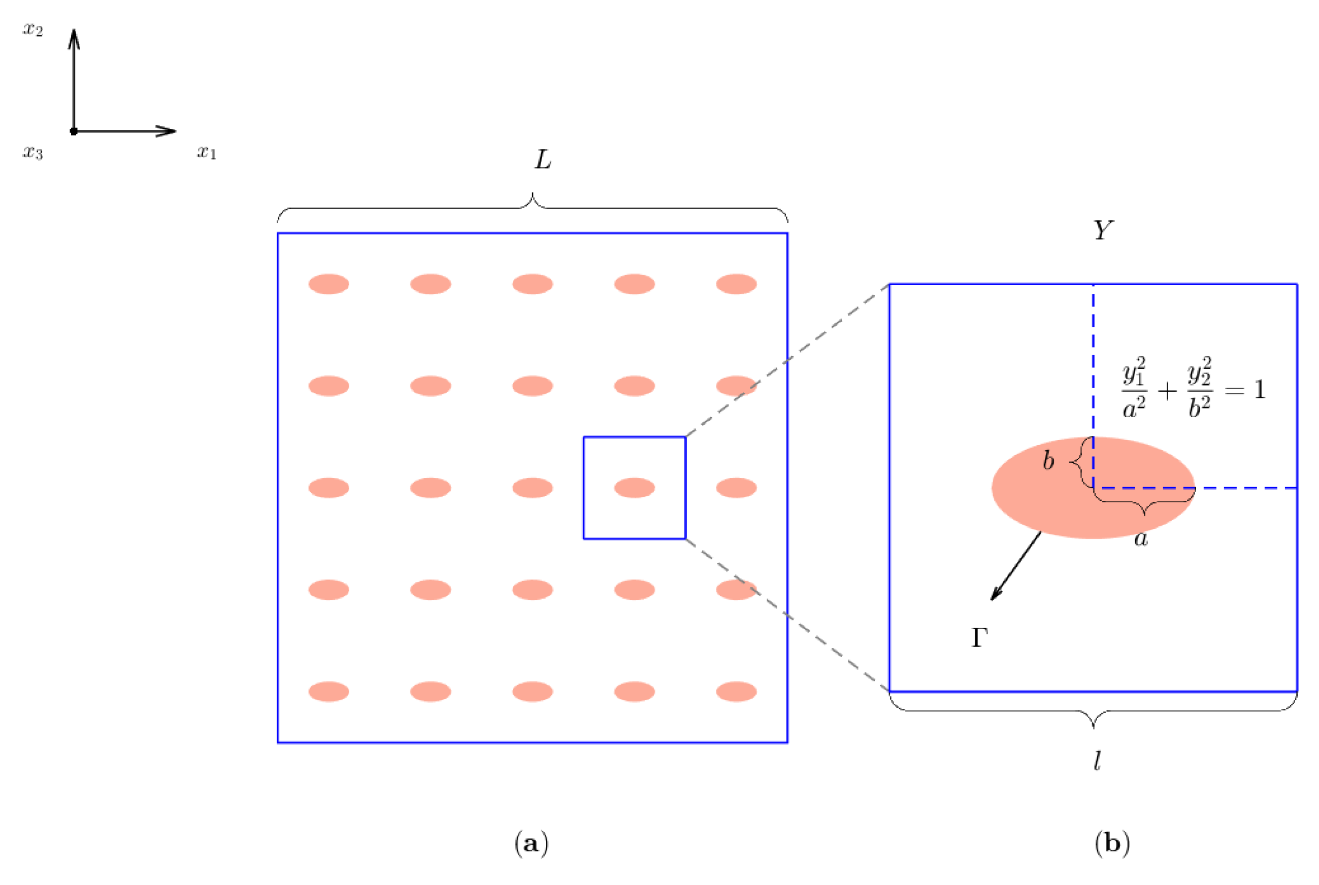
We consider a two-phase uniaxial reinforced material where the fibers and matrix have isotropic or transversely isotropic thermoelastic properties. Let the position of a typical point of the body be denoted by three coordinates $(x_1,x_2,x_3)$ in a Cartesian system of coordinates. Axis $x_3$ corresponds to the axis of transverse symmetry which points along the direction of the fiber. Additionally, the fibers are periodically distributed along the directions of the axes $x_1$ and $x_2$. 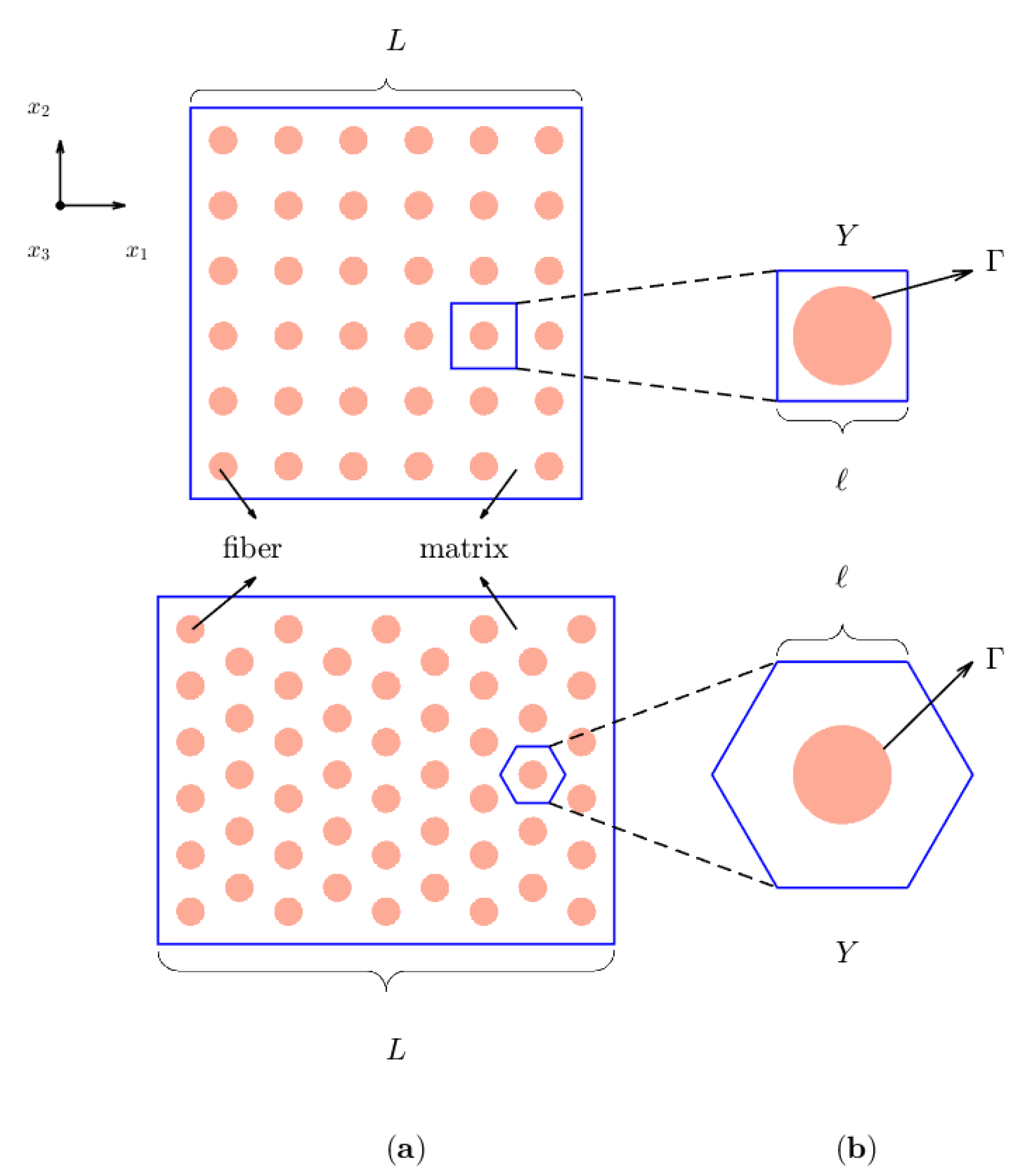Figure 1a illustrates the fiber distribution for square (up) and hexagonal (down) cells.

The characteristic size ℓ of the inhomogeneities is assumed to be much smaller than the global size L of the whole structure ($\ell \ll L$). The AHM is used to solve the problem. The AHM allows to determine the effective properties of composite materials from a double-scale asymptotic development. The study of the initial problem in a heterogeneous medium (Figure 1a) becomes an equivalent problem in a homogeneous medium. The problem in the homogeneous medium requires the solution of local problems on a representative cell of the material: the periodic cell Y. Figure 1b represents the periodic cell for the square (up) and the hexagonal (down) distributions. A dimensionless small parameter $ϵ=\raisebox{1ex}{$\ell $}\!\left/ \!\raisebox{-1ex}{$L$}\right.$, $ϵ\ll 1$ characterizing the rate of heterogeneity of the composite structure is introduced. In order to separate the micro and macroscale components of the solution, the so-called slow ($x_i$) and fast ($y_i$) coordinates are also introduced

$$y_i=\frac{x_i}{ϵ},i=1,2,3.$$

(1)

The fast variable $y_i$ represents the rapid change of properties of the composite or the degree of the heterogeneity.

The linear equation of equilibrium in the quasi-static and stationary problem is given by

$${\sigma }_{ij,j}+X_i=0,$$

(2)

where the subscripts assume the values $1,2$ and 3; the comma denotes partial differentiation and the summation convention is applied; the body forces are represented by $X_i$; and $\sigma$ is the stress tensor. The stress ($\sigma$) and strain ($\epsilon$) tensors are related to the temperature change ($\theta$) by the constitutive relations also known as the Duhamel–Neumann law [8]

$$\begin{array}{ccc}\hfill {\sigma }_{ij}\left(\mathbf{x}\right)& =& {\mathit{C}}_{ijkl}\left(\mathbf{y}\right){\epsilon }_{kl}\left(\mathbf{x}\right)-{\mathit{\beta }}_{ij}\left(\mathbf{y}\right)\theta \left(\mathbf{x}\right),\hfill \end{array}$$

(3)

$$\begin{array}{ccc}\hfill {\mathit{\beta }}_{ij}\left(\mathbf{y}\right)& =& {\mathit{C}}_{ijkl}\left(\mathbf{y}\right){\mathit{\alpha }}_{kl}\left(\mathbf{y}\right),\hfill \end{array}$$

(4)

where $\mathbf{x}=(x_1,x_2,x_3)$ and $\mathbf{y}=(y_1,y_2,y_3)$. The constitutive laws contain the components of the elasticity fourth-order tensor ${\mathit{C}}_{ijkl}\left(\mathbf{y}\right)$, the components of the thermal stress second-order tensor ${\mathit{\beta }}_{ij}\left(\mathbf{y}\right)$ and ${\mathit{\alpha }}_{kl}\left(\mathbf{y}\right)$, which represent the thermal expansion coefficients. The strain tensor is defined by the Cauchy relations

$${\epsilon }_{kl}\left(\mathbf{x}\right)=\frac{u_{k,l}\left(\mathbf{x}\right)+u_{l,k}\left(\mathbf{x}\right)}{2},$$

(5)

where $u_k$ are the components of the displacement. The heat flow vector is expressed in terms of the temperature as stated by Fourier’s law

$$q_i=-{\mathit{\kappa }}_{ij}\left(\mathbf{y}\right){\theta }_{,j}\left(\mathbf{x}\right),$$

(6)

where ${\mathit{\kappa }}_{ij}\left(\mathbf{y}\right)$ denotes the thermal conductivity components. Using Equation (6), the heat balance equation is written as follows [25]

$$q_{i,i}(\mathbf{x},t)=-{\left({\mathit{\kappa }}_{ij}\left(\mathbf{y}\right){\theta }_{,j}\left(\mathbf{x}\right)\right)}_{,i}=f\left(\mathbf{x}\right),$$

(7)

where f is the density of the internal heat sources. Equations (2)–(7) form a coupled linear system of thermoelasticity equations with rapidly oscillating coefficients for an anisotropic inhomogeneous solid. Appropriate boundary and initial conditions should be specified for this system. All coefficients ${\mathit{C}}_{ijkl}$, ${\mathit{\beta }}_{ij}$, ${\mathit{\alpha }}_{ij}$ and ${\mathit{\kappa }}_{ij}$ are considered to be picewise-smooth Y-periodic functions of the fast coordinates $y_i$.

The idea of the homogenization approach is to obtain a closed system of equations with constant coefficients, equivalent to the system given by Equation (2)–(7). These new coefficients are considered to represent the global properties of the composite. Through the AHM [8], the original constitutive relations with rapidly oscillating material coefficients are transformed in two sets of mathematical problems. The first set has new physical relations over Y with constant coefficients $\overline{\mathit{C}}$, $\overline{\mathit{\beta }}$ and $\overline{\mathit{\kappa }}$ which represent the properties of an equivalent homogeneous medium, and they are called the effective coefficients of the composite. They are calculated by using the following relations [8]

$$\begin{array}{ccc}\hfill {\overline{\mathit{C}}}_{ijpq}& =& 〈{\mathit{C}}_{ijpq}\left(\mathbf{y}\right)+{\mathit{C}}_{ijkl}\left(\mathbf{y}\right){}_{pq}{\mathrm{U}}_{k,l}\left(\mathbf{y}\right)〉,\hfill \end{array}$$

(8)

$$\begin{array}{ccc}\hfill {\overline{\mathit{\beta }}}_{ij}& =& 〈{\mathit{\beta }}_{ij}\left(\mathbf{y}\right)-{\mathit{C}}_{ijkl}\left(\mathbf{y}\right){}_{pp}{R}_{k,l}\left(\mathbf{y}\right)〉,\hfill \end{array}$$

(9)

$$\begin{array}{ccc}\hfill {\overline{\mathit{\kappa }}}_{iq}& =& 〈{\mathit{\kappa }}_{iq}\left(\mathbf{y}\right)+{\mathit{\kappa }}_{ik}\left(\mathbf{y}\right){}_q{M}_{,k}\left(\mathbf{y}\right)〉,\hfill \end{array}$$

(10)

where $〈*〉$ represents the average operator such that $〈f〉=\frac{{\int }_{Y}fdY}{\left|Y\right|}$, and the subscripts $i,j,k,l,p$ and q assume the values $1,2$ and 3. Equation (8) shows that the effective elastic coefficients can be obtained in the same manner for elastic [10] and thermoelastic materials.

The second set of resulting problems from the AHM allows the calculation of the functions, ${}_{pq}{\mathrm{U}}_k\left(\mathbf{y}\right)$, ${}_{pp}{R}_k\left(\mathbf{y}\right)$ and ${}_{q}M\left(\mathbf{y}\right)$ which are solutions of the so-called local problems. The local problems for the elastic (${}_{pq}L$) and thermal (${}_{pp}T$, ${}_{q}I$) problems are solved over the periodic cell Y and they were derived in ref. [8] as

$$\begin{array}{ccc}\hfill {({\mathit{C}}_{ijpq}\left(\mathbf{y}\right)+{\mathit{C}}_{ijkl}\left(\mathbf{y}\right){}_{pq}{\mathrm{U}}_{k,l}\left(\mathbf{y}\right))}_{,j}& =& 0,\hfill \end{array}$$

(11)

$$\begin{array}{ccc}\hfill {({\mathit{\beta }}_{ij}\left(\mathbf{y}\right)-{\mathit{C}}_{ijkl}\left(\mathbf{y}\right){}_{pp}{R}_{k,l}\left(\mathbf{y}\right))}_{,j}& =& 0,\hfill \end{array}$$

(12)

$$\begin{array}{ccc}\hfill {({\mathit{\kappa }}_{ij}\left(\mathbf{y}\right)+{\mathit{\kappa }}_{ik}\left(\mathbf{y}\right){}_q{M}_{,k}\left(\mathbf{y}\right))}_{,i}& =& 0,\hfill \end{array}$$

(13)

with perfect contact conditions at the interface $\mathsf{\Gamma }$ shown as

$$\begin{array}{c}{\left|\left|{}_{pq}{\mathrm{U}}_i\right|\right|}_{\mathsf{\Gamma }}=0,{\left|\left|({\mathit{C}}_{ijpq}+{\mathit{C}}_{ijkl}{}_{pq}{\mathrm{U}}_{k,l}){\mathrm{n}}_j\right|\right|}_{\mathsf{\Gamma }}=0,\\ {\left|\left|{}_{pp}{R}_i\right|\right|}_{\mathsf{\Gamma }}=0,{\left|\left|({\mathit{\beta }}_{ij}-{\mathit{C}}_{ijkl}{}_{pp}{R}_{k,l}){\mathrm{n}}_j\right|\right|}_{\mathsf{\Gamma }}=0,\\ {\left|\left|{}_{q}M\right|\right|}_{\mathsf{\Gamma }}=0,{\left|\left|({\mathit{\kappa }}_{iq}+{\mathit{\kappa }}_{ik}{}_q{M}_{,k}){\mathrm{n}}_i\right|\right|}_{\mathsf{\Gamma }}=0.\end{array}$$

(14)

The vector $\mathbf{n}$ represents the outward unit normal vector to the interface $\mathsf{\Gamma }$ and ${\mathrm{n}}_{\mathrm{j}}$ are the vector’s components. The discontinuity of the function g through the interface is denoted by $\left|\right|g\left|\right|$, and ${}_{pq}{\mathrm{U}}_k\left(\mathbf{y}\right)$, ${}_{pp}{R}_k\left(\mathbf{y}\right)$ and ${}_{q}M\left(\mathbf{y}\right)$ constitute the $Y-$periodic functions related to the mechanical displacements, the thermal stress tensor and thermal conductivity, respectively. The material coefficients ${\mathit{C}}_{ijpq}\left(\mathbf{y}\right)$, ${\mathit{\beta }}_{ij}\left(\mathbf{y}\right)$ and ${\mathit{\kappa }}_{ij}\left(\mathbf{y}\right)$ are known functions of the constituent phases in the local variable $\mathbf{y}$ on the periodic cell Y. More details explaining the AHM procedure and the mathematical background can be found in the classical works [13,26,27,28]. Considering only $\raisebox{1ex}{$1$}\!\left/ \!\raisebox{-1ex}{$4$}\right.$ of the periodic cell’s surface to perform the calculations, the periodic boundary conditions must be transformed into mixed boundary conditions as illustrated in Appendix A.

Table 1. Relationship between the local problems and the effective properties.

${}_{11}\mathit{L}$	${}_{22}\mathit{L}$	${}_{33}\mathit{L}$	${}_{23}\mathit{L}$	${}_{13}\mathit{L}$	${}_{12}\mathit{L}$	${}_{11}\mathit{T}$	${}_1\mathit{I}$	${}_2\mathit{I}$	${}_3\mathit{I}$
${\overline{C}}_{1111}$	${\overline{C}}_{1122}$	${\overline{C}}_{1133}$	${\overline{C}}_{2323}$	${\overline{C}}_{1313}$	${\overline{C}}_{1212}$	${\overline{\mathit{\beta }}}_{11}$	${\overline{\mathit{\kappa }}}_{11}$	${\overline{\mathit{\kappa }}}_{22}$	${\overline{\mathit{\kappa }}}_{33}$
${\overline{C}}_{2211}$	${\overline{C}}_{2222}$	${\overline{C}}_{2233}$	-	-	-	${\overline{\mathit{\beta }}}_{22}$	-	-	-
${\overline{C}}_{3311}$	${\overline{C}}_{3322}$	${\overline{C}}_{3333}$	-	-	-	${\overline{\mathit{\beta }}}_{33}$	-	-	-

shows the relationship between the local problems and the effective properties obtained through their solution.

Given the existing symmetry between p and q, there are just six non-homogeneous local problems ${}_{pq}L$ that contribute to the estimation of the effective elastic properties: the plane problems ${}_{11}L$, ${}_{12}L$, ${}_{22}L$, ${}_{33}L$ and the anti-plane problems ${}_{13}L$, ${}_{23}L$. The expressions to compute the elastic coefficients ${\overline{\mathit{C}}}_{ijkl}$ are obtained from Equation (8)

$$\begin{array}{ccc}\hfill {\overline{C}}_{1111}& =& \frac{4}{A}\int {\int }_{\Omega }\left(C_{1111}+C_{1111}{}_{11}{\mathrm{U}}_{1,1}+C_{1122}{}_{11}{\mathrm{U}}_{2,2}\right)d\Omega ,\hfill \\ \hfill {\overline{C}}_{1122}={\overline{C}}_{2211}& =& \frac{4}{A}\int {\int }_{\Omega }\left(C_{1122}+C_{1111}{}_{22}{\mathrm{U}}_{1,1}+C_{1122}{}_{22}{\mathrm{U}}_{2,2}\right)d\Omega ,\hfill \\ \hfill {\overline{C}}_{2222}& =& \frac{4}{A}\int {\int }_{\Omega }\left(C_{2222}+C_{1122}{}_{22}{\mathrm{U}}_{1,1}+C_{2222}{}_{22}{\mathrm{U}}_{2,2}\right)d\Omega ,\hfill \\ \hfill {\overline{C}}_{1133}={\overline{C}}_{3311}& =& \frac{4}{A}\int {\int }_{\Omega }\left(C_{1133}+C_{1111}{}_{33}{\mathrm{U}}_{1,1}+C_{1122}{}_{33}{\mathrm{U}}_{2,2}\right)d\Omega ,\hfill \\ \hfill {\overline{C}}_{2233}={\overline{C}}_{3322}& =& \frac{4}{A}\int {\int }_{\Omega }\left(C_{2233}+C_{2211}{}_{33}{\mathrm{U}}_{1,1}+C_{2222}{}_{33}{\mathrm{U}}_{2,2}\right)d\Omega ,\hfill \\ \hfill {\overline{C}}_{3333}& =& \frac{4}{A}\int {\int }_{\Omega }\left(C_{3333}+C_{3311}{}_{33}{\mathrm{U}}_{1,1}+C_{3322}{}_{33}{\mathrm{U}}_{2,2}\right)d\Omega ,\hfill \\ \hfill {\overline{C}}_{2323}& =& \frac{4}{A}\int {\int }_{\Omega }\left(C_{2323}+C_{2323}{}_{23}{\mathrm{U}}_{3,2}\right)d\Omega ,\hfill \\ \hfill {\overline{C}}_{1313}& =& \frac{4}{A}\int {\int }_{\Omega }\left(C_{1313}+C_{1313}{}_{13}{\mathrm{U}}_{3,1}\right)d\Omega ,\hfill \\ \hfill {\overline{C}}_{1212}& =& \frac{4}{A}\int {\int }_{\Omega }{C}_{1212}\left(1+{}_{12}{\mathrm{U}}_{1,2}+{}_{12}{\mathrm{U}}_{2,1}\right)d\Omega ,\hfill \end{array}$$

(15)

where $\Omega$ represents the periodic cell and A corresponds to the cell’s area.

Thermal problems ${}_{pp}T$ are mathematically analogous to purely elastic plane problems. The solutions obtained from problem ${}_{11}T$ are sufficient to determine the effective coefficients ${\overline{\mathit{\beta }}}_{11}$, ${\overline{\mathit{\beta }}}_{22}$ and ${\overline{\mathit{\beta }}}_{33}$. Therefore, it is only necessary to solve the differential equations that result from the local problem ${}_{11}T$. The effective values of the thermal stress tensor ${\overline{\mathit{\beta }}}_{ij}$ are derived from Equation (9) and they can be obtained as

$$\begin{array}{ccc}\hfill {\overline{\mathit{\beta }}}_{11}& =& \frac{4}{A}\int {\int }_{\Omega }({\mathit{\beta }}_{11}-(C_{1111}{}_{11}{R}_{1,1}+C_{1122}{}_{11}{R}_{2,2}))d\Omega ,\hfill \\ \hfill {\overline{\mathit{\beta }}}_{22}& =& \frac{4}{A}\int {\int }_{\Omega }({\mathit{\beta }}_{22}-(C_{2211}{}_{22}{R}_{1,1}+C_{2222}{}_{22}{R}_{2,2}))d\Omega ,\hfill \\ \hfill {\overline{\mathit{\beta }}}_{33}& =& \frac{4}{A}\int {\int }_{\Omega }({\mathit{\beta }}_{33}-(C_{3311}{}_{33}{R}_{1,1}+C_{3322}{}_{33}{R}_{2,2}))d\Omega .\hfill \end{array}$$

(16)

Once the $\overline{\mathit{C}}$ and the $\overline{\mathit{\beta }}$ coefficients have been calculated, it is possible to obtain the effective thermal expansion coefficients $\overline{\mathit{\alpha }}$ through Equation (4).

For thermal capacity problems ${}_{q}I$, it can be deduced that problems ${}_{1}I$ and ${}_{2}I$ are analogous to purely elastic anti-plane problems. From Equation (10) it follows that ${\overline{\mathit{\kappa }}}_{33}$ is consistent with the Voigt average [8]. The effective thermal conductivity is derived from Equation (10) and can be estimated as follows

$$\begin{array}{ccc}\hfill {\overline{\mathit{\kappa }}}_{11}& =& \frac{4}{A}\int {\int }_{\Omega }({\mathit{\kappa }}_{11}+{\mathit{\kappa }}_{11}{}_1{M}_{,1})d\Omega ,\hfill \\ \hfill {\overline{\mathit{\kappa }}}_{22}& =& \frac{4}{A}\int {\int }_{\Omega }({\mathit{\kappa }}_{22}+{\mathit{\kappa }}_{22}{}_2{M}_{,2})d\Omega ,\hfill \\ \hfill {\overline{\mathit{\kappa }}}_{33}& =& \frac{4}{A}\int {\int }_{\Omega }{\mathit{\kappa }}_{33}d\Omega .\hfill \end{array}$$

(17)

3. Finite Element Method

The thermoelastic effective properties are given by Equation (8)–(10). Additionally, to calculate the effective coefficients it is necessary to solve the local problems given by Equation (11)–(13) to obtain the values: ${}_{pq}{\mathrm{U}}_{k,l}\left(\mathbf{y}\right)$, ${}_{pp}{R}_{k,l}\left(\mathbf{y}\right)$ and ${}_q{M}_{,k}\left(\mathbf{y}\right)$. The FEM is one of the most popular numerical methods used to solve differential equations [29]. The region of interest must be discretized into elements in order to apply the FEM. The strong formulation of the differential problem is transformed into a weak formulation or integral problem. The matrix formulation is obtained on each element and then it is assembled into a global system of equations. The shape functions are chosen and incorporated into the formulation. Finally, the resulting system of equations is solved.

The composite material is formed by a matrix with cylindrical fibers periodically distributed in the $x_3$ direction as mentioned previously. This makes it possible to reduce the problem into a two-dimensional problem. The region of interest will be the periodic cell, since the fibers are periodically distributed. In this work, square and hexagonal cells are studied, as shown in Figure 1a.

Since the representative cell has a symmetric geometry, calculations are performed using only $\raisebox{1ex}{$1$}\!\left/ \!\raisebox{-1ex}{$4$}\right.$ of the cell, which reduces significantly the number of operations and CPU time. In this section, a finite element formulation is performed to solve differential Equations (12) and (13) for the ${}_{1}I$ and ${}_{11}T$ local problems. The remaining local problems are implemented in a similar fashion.

3.1. Discretization of the Region

The first step in the FEM implementation is to discretize the region where the differential equation is to be solved, which corresponds to the quarter of the cell. For the square distribution, let us assume that the periodic cell is 1 unit long; therefore, the width and height of the quarter square cell are $0.5$ units long. The symmetric quarter of the cell corresponding to a hexagonal distribution is made of one rectangle and two quarters of fibers. The hexagon’s side length is assumed to be 1 unit, so the width of the periodical hexagonal cell is $\raisebox{1ex}{$3$}\!\left/ \!\raisebox{-1ex}{$4$}\right.$ units and its height is equal to $\raisebox{1ex}{$\sqrt{3}$}\!\left/ \!\raisebox{-1ex}{$4$}\right.$ units. The $(0,0)$ coordinate is located in the lower left corner of the cell in both cases.

In this work, the meshes that represent the quarter of the cell are automatically generated. The method described in ref. [30] was used to construct these meshes. First, a description of the geometry to be discretized is provided. In order to generate the initial geometry of the cell, the user must specify the radius of the fiber and the number of elements that the final mesh will have in the $y_2$ direction. Once these two parameters are defined, the initial blocks are created. Blocks are 8-node quadrilaterals that discretize the region. Each block is made of a single material. The number of subdivisions to be performed in the $y_1$ and $y_2$ directions is defined for each block. Additionally, if there are elements with curved sides, then for each of those elements, the coordinates of a point located close to the middle section and over the curved side must be specified. The connectivity of the blocks must also be defined, which is the way in which the nodes that constitute a specific block are related.

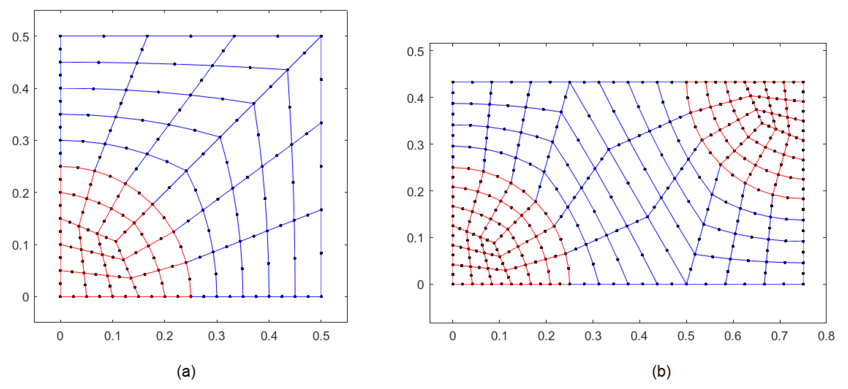
Once the initial geometry has been determined, the corresponding mesh is generated. The correspondence between a block and the parent element must be established in order to generate the corresponding mesh. This correspondence can be achieved through the same isoparametric representation that will be used later during the FEM formulation. Figure 2a,b show the meshes obtained using the method described in ref. [30] for square and hexagonal cells, respectively.

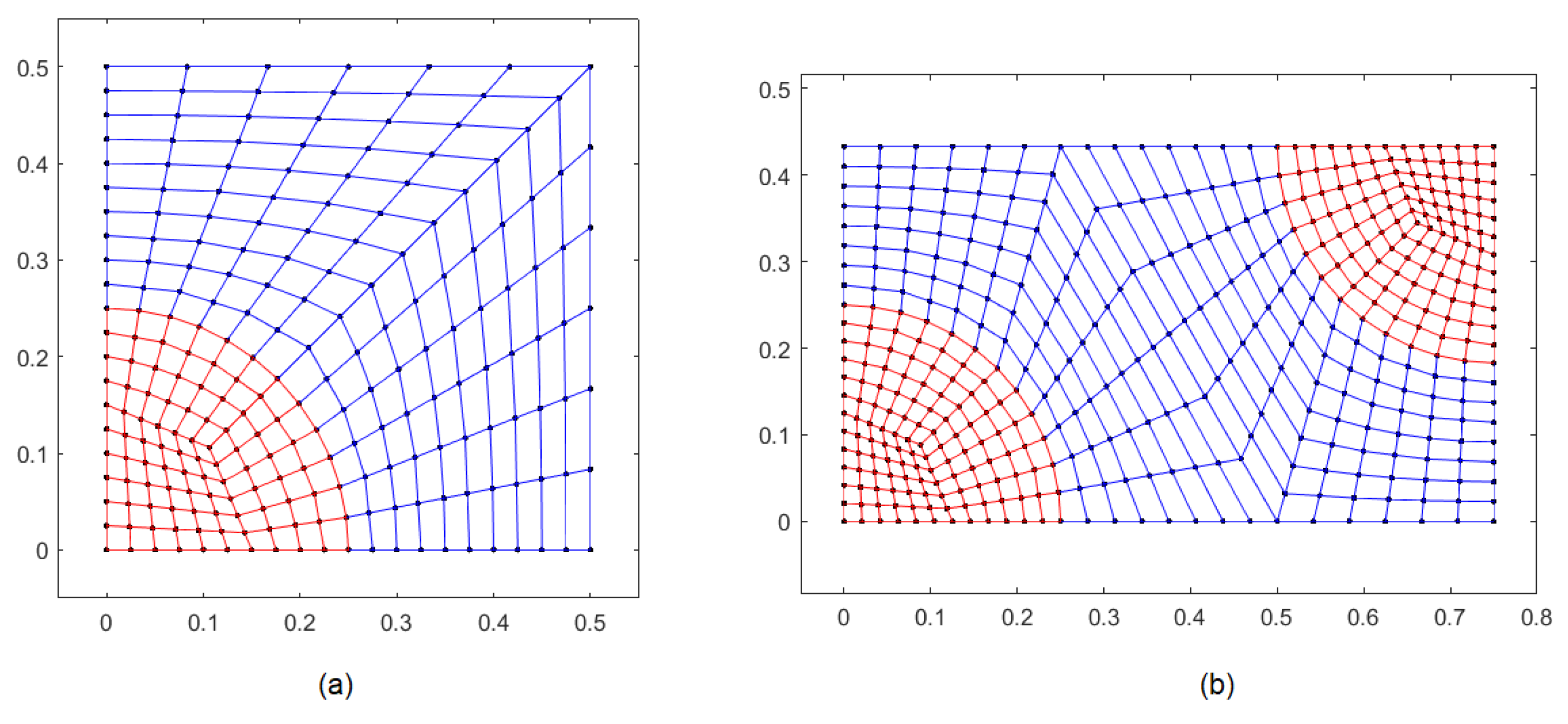
Linear and quadratic FEM formulations are carried out throughout this investigation. Thus, one more step must be performed to obtain the 4-node quadrilateral mesh when solving the problem by using the linear FEM formulation. The 8-node mesh should be transformed into a 4-node mesh, through division of each 8-node element into four 4-node elements. Figure 3a,b show the meshes obtained by transforming the 8-node quadrilateral meshes presented in Figure 2a,b, respectively.

Let $\Omega$ be the region where the differential problem must be solved. The region $\Omega$ is represented by the mesh previously determined.

3.2. Shape Functions

As mentioned in Section 3.1, the region $\Omega$ is divided into a finite number of quadrilateral elements. Two types of quadrilateral elements are used: 4-node quadrilateral elements (linear case) and 8-node quadrilateral elements (quadratic case).

The main idea of the FEM is to approximate the unknown function at each discretized element using some approximation functions (also known as shape functions). Once the shape functions have been chosen, they are incorporated into the problem’s formulation. There are many ways to choose a set of functions that form a vector basis on which to approximate the exact solution of the problem. Lagrange functions are the most common type of shape functions in the FEM. These functions are piecewise polynomials defined at each element e. In this work, linear and quadratic Lagrange shape functions are used. Therefore, in the linear case, each element will have 4 nodes, while in the quadratic case each element will have 8 nodes. Expressions for the linear and quadratic Lagrange shape functions can be found in ref. [29]. Let $\mathbf{N}=\{N_1{N}_2\cdots N_n\}$ with $n=4,8$ be the basis of the Lagrange functions in the space where we seek to approximate the solution.

The elements of the mesh that are used to discretize the region $\Omega$ are defined by the local coordinates $(y_1,y_2)$. However, the shape functions are generally defined in parent coordinates $(\xi ,\eta )$. Therefore, it is necessary to perform a transformation from local coordinates to parent coordinates and vice versa. The transformation from local coordinates $(y_1,y_2)$ to parent coordinates $(\xi ,\eta )$ obeys the following mapping

$$\begin{array}{ccc}\hfill y_1(\xi ,\eta )& =& \mathbf{N}(\xi ,\eta ){\mathbf{y}}_1^e,\hfill \\ \hfill y_2(\xi ,\eta )& =& \mathbf{N}(\xi ,\eta ){\mathbf{y}}_2^e,\hfill \end{array}$$

(18)

where vectors ${\mathbf{y}}_1^e={\left[y_{11},y_{12},...,y_{1n}\right]}^t$ and ${\mathbf{y}}_2^e={\left[y_{21},y_{22},...,y_{2n}\right]}^t$ are the known nodal coordinates of the element, and $n=4$ ($n=8$) has been used for the linear (quadratic) case. Using expressions (18) and the chain rule, the $\xi$ and $\eta$ derivatives of the ith shape function could be expressed in terms of the $y_1$ and $y_2$ derivatives as follows

$$\begin{array}{ccc}\hfill \frac{\partial N_i}{\partial \xi }& =& \frac{\partial N_i}{\partial y_1}\frac{\partial y_1}{\partial \xi }+\frac{\partial N_i}{\partial y_2}\frac{\partial y_2}{\partial \xi },\hfill \\ \hfill \frac{\partial N_i}{\partial \eta }& =& \frac{\partial N_i}{\partial y_1}\frac{\partial y_1}{\partial \eta }+\frac{\partial N_i}{\partial y_2}\frac{\partial y_2}{\partial \eta }.\hfill \end{array}$$

(19)

Equation (19) can be written in a more compact form as

$$\begin{array}{ccc}\hfill \left[\begin{array}{c}\frac{\partial N_i}{\partial \xi }\\ \frac{\partial N_i}{\partial \eta }\end{array}\right]& =& \mathbf{J}\left[\begin{array}{c}\frac{\partial N_i}{\partial y_1}\\ \frac{\partial N_i}{\partial y_2}\end{array}\right],\hfill \end{array}$$

(20)

where

$$\mathbf{J}=\left[\begin{array}{cc}{J}_{11}& J_{12}\\ J_{21}& J_{22}\end{array}\right]=\left[\begin{array}{cc}\frac{\partial y_1}{\partial \xi }& \frac{\partial y_2}{\partial \xi }\\ \frac{\partial y_1}{\partial \eta }& \frac{\partial y_2}{\partial \eta }\end{array}\right],$$

(21)

is the Jacobian matrix. The Jacobian matrix is shown below for an n-node element ($n=4$ or $n=8$)

$$\mathbf{J}=\left[\begin{array}{cccc}\frac{\partial N_1}{\partial \xi }& \frac{\partial N_2}{\partial \xi }& ...& \frac{\partial N_n}{\partial \xi }\\ \frac{\partial N_1}{\partial \eta }& \frac{\partial N_2}{\partial \eta }& ...& \frac{\partial N_n}{\partial \eta }\end{array}\right]\left[\begin{array}{cc}{y}_{11}& y_{21}\\ y_{12}& y_{22}\\ ⋮& ⋮\\ y_{1n}& y_{2n}\end{array}\right].$$

(22)

In general, each element of the discretization has a different Jacobian matrix, and entries of the Jacobian matrices are functions of $(\xi ,\eta )$.

When the Jacobian determinant $\left|\mathbf{J}\right|$ is positive at any point in the region, it is possible to invert the transformation in order to determine $\xi (y_1,y_2)$ and $\eta (y_1,y_2)$. This possibility means that for a given point $(y_1,y_2)$ within the quadrilateral element, there is a single point $(\xi ,\eta )$ in the parent element. Provided that the transformation is invertible, the following can be written

$$\begin{array}{ccc}\hfill \left[\begin{array}{c}\frac{\partial N_i}{\partial y_1}\\ \frac{\partial N_i}{\partial y_2}\end{array}\right]& =& {\mathbf{J}}^{-1}\left[\begin{array}{c}\frac{\partial N_i}{\partial \xi }\\ \frac{\partial N_i}{\partial \eta }\end{array}\right],\hfill \end{array}$$

(23)

where ${\mathbf{J}}^{-1}$ is the inverse of the Jacobian matrix. Additionally, the surface differentials at each coordinate system are related as follows

$$d{\Omega }^e=d{y}_{1}d{y}_2=\left|\mathbf{J}\right|d\xi d\eta .$$

(24)

3.3. The ${}_{1}I$ Local Problem: Weak Formulation

The differential equation used to calculate the thermal conductivity for the problem ${}_{1}I$ can be obtained from Equation (13) and it is given by

$${({\mathit{\kappa }}_{11}+{\mathit{\kappa }}_{11}{}_1{M}_{,1})}_{,1}+{\left({\mathit{\kappa }}_{22}{}_1{M}_{,2}\right)}_{,2}=0.$$

(25)

Perfect contact conditions (14) for problem $qI$ are given by

$$\begin{array}{ccc}\hfill {\left|\left|\left({\mathit{\kappa }}_{11}+{\mathit{\kappa }}_{11}{}_1{M}_{,1}\right){\mathrm{n}}_1+{\mathit{\kappa }}_{22}{}_1{M}_{,2}{\mathrm{n}}_2\right|\right|}_{\mathsf{\Gamma }}& =& 0,\hfill \\ \hfill {\left|\left|{\mathit{\kappa }}_{11}{\mathrm{n}}_1+{\tau }_{11}{\mathrm{n}}_1+{\tau }_{22}{\mathrm{n}}_2\right|\right|}_{\mathsf{\Gamma }}& =& 0,\hfill \\ \hfill {\left|\left|{\tau }_{11}{\mathrm{n}}_1+{\tau }_{22}{\mathrm{n}}_2\right|\right|}_{\mathsf{\Gamma }}& =& -{\left|\left|{\mathit{\kappa }}_{11}{\mathrm{n}}_1\right|\right|}_{\mathsf{\Gamma }},\hfill \end{array}$$

(26)

where ${\tau }_{11}={\mathit{\kappa }}_{11}{}_1{M}_{,1}$, ${\tau }_{22}={\mathit{\kappa }}_{22}{}_1{M}_{,2}$ and $\left|\left|g\right|\right|$ denotes the discontinuity or jump of the function g across the interface. The jump at the interface $\mathsf{\Gamma }$ for the conductivity problem is defined by

$${\left|\left|{\mathit{\kappa }}_{11}{\mathrm{n}}_1\right|\right|}_{\mathsf{\Gamma }}=({\mathit{\kappa }}_{11}^m-{\mathit{\kappa }}_{11}^f){\mathrm{n}}_1,$$

where ${\mathit{\kappa }}_{11}^m$ and ${\mathit{\kappa }}_{11}^f$ are the matrix and fiber thermal conductivity ${\mathit{\kappa }}_{11}$ coefficient, respectively. By using symmetry and periodicity conditions, the boundary conditions for problem ${}_{1}I$ are obtained

$$\begin{array}{ccc}\hfill {}_{1}M=0,& \mathrm{in}\partial {\Omega }_L,{}_{1}M=0,& \mathrm{in}\partial {\Omega }_R,\hfill \\ \hfill {}_1{\tau }_2=0,& \mathrm{in}\partial {\Omega }_U,{}_1{\tau }_2=0,& \mathrm{in}\partial {\Omega }_D,\hfill \end{array}$$

where $\partial {\Omega }_L$, $\partial {\Omega }_R$, $\partial {\Omega }_U$ and $\partial {\Omega }_D$ represent the left, right, upper and lower boundaries of the cell quarter.

Assuming that we look for the approximate solution $\tilde{M}\approx M$ of the problem (25) within a certain space of functions $\mathcal{H}$ with dimension n,

$$\tilde{M}=\mathbf{Nq},$$

(27)

where $\mathbf{N}=\left[N_1{N}_2\cdots N_n\right]$ is a basis of $\mathcal{H}$ and $\mathbf{q}={[q_1{q}_2\cdots q_n]}^t$ are the nodal values of the unknown field. The weak formulation of problem ${}_{1}I$ is obtained by applying the weighted residual method and Galerkin’s method [30,31]. The differential problem (25) becomes

$$\begin{array}{ccc}\hfill \sum _{e=1}^n\int {\int }_{{\Omega }^e}{\mathbf{D}}^t\mathbf{C}\mathbf{D}d{\Omega }^e\mathbf{q}& =& \sum _{e=1}^n\int {\int }_{{\Omega }^e}\frac{\partial {\mathit{\kappa }}_{11}}{\partial y_1}{\mathbf{N}}^{t}d{\Omega }^e+\sum _{e=1}^n{\oint }_{{\mathsf{\Gamma }}^e}({\tilde{\tau }}_{11}{\mathrm{n}}_1+{\tilde{\tau }}_{22}{\mathrm{n}}_2){\mathbf{N}}^{t}d{\mathsf{\Gamma }}^e,\hfill \end{array}$$

(28)

where

$$\begin{array}{ccc}\hfill \mathbf{D}=\left(\begin{array}{c}\frac{\partial \mathbf{N}}{\partial y_1}\\ \frac{\partial \mathbf{N}}{\partial y_2}\end{array}\right),& & \mathbf{C}=\left[\begin{array}{cc}{\mathit{\kappa }}_{11}& 0\\ 0& {\mathit{\kappa }}_{22}\end{array}\right],\hfill \\ \hfill {\tilde{\tau }}_{11}={\mathit{\kappa }}_{11}\frac{\partial \tilde{M}}{\partial y_1},& & {\tilde{\tau }}_{22}={\mathit{\kappa }}_{22}\frac{\partial \tilde{M}}{\partial y_2},\hfill \end{array}$$

${\tilde{\tau }}_{11}$ and ${\tilde{\tau }}_{22}$ represent the jump between different materials at the interface $\mathsf{\Gamma }$ and ${\mathrm{n}}_1,{\mathrm{n}}_2$ constitute the components of the unitary normal vector at the interface. The stiffness matrix, the force vector and the traction at the boundary of each element can be obtained from Equation (28)

$$\begin{array}{ccc}\hfill {\mathbf{K}}^e& =& \int {\int }_{{\Omega }^e}{\mathbf{D}}^t\mathbf{C}\mathbf{D}d{\Omega }^e,\hfill \end{array}$$

(29)

$$\begin{array}{ccc}\hfill {\mathbf{F}}^e& =& \int {\int }_{{\Omega }^e}\frac{\partial {\mathit{\kappa }}_{11}}{\partial y_1}{\mathbf{N}}^{t}d{\Omega }^e,\hfill \end{array}$$

(30)

$$\begin{array}{ccc}\hfill {\mathbf{B}}^e& =& {\oint }_{{\mathsf{\Gamma }}^e}({\tilde{\tau }}_{11}{\mathrm{n}}_1+{\tilde{\tau }}_{22}{\mathrm{n}}_2){\mathbf{N}}^{t}d{\mathsf{\Gamma }}^e.\hfill \end{array}$$

(31)

Expressions (29)–(31) are the element stiffness matrix, the element force vector and the integral vector that corresponds to the boundary of each element. The vector ${\mathbf{B}}^e$ must be evaluated only at the edges that belong to the interface $\mathsf{\Gamma }$. Equation (26) is used to determine the vector ${\mathbf{B}}^e$. Once the matrices and vectors of each element have been calculated, they are assembled to form the global system of equations which results in the following expression

$$\mathbf{Kq}=\mathbf{F}+\mathbf{B}.$$

(32)

3.4. The ${}_{11}T$ Local Problem: Weak Formulation

The system of differential equations that defines the problem ${}_{11}T$ is given by

$$\begin{array}{c}\hfill {\left({\mathit{\beta }}_{11}-C_{1111}{}_{11}{R}_{1,1}-C_{1122}{}_{11}{R}_{2,2}\right)}_{,1}-{\left(C_{1212}{}_{11}{R}_{1,2}+C_{1212}{}_{11}{R}_{2,1}\right)}_{,2}=0,\\ \hfill -{\left(C_{1212}{}_{11}{R}_{1,2}+C_{1212}{}_{11}{R}_{2,1}\right)}_{,1}+{\left({\mathit{\beta }}_{22}-C_{1122}{}_{11}{R}_{1,1}-C_{2222}{}_{11}{R}_{2,2}\right)}_{,2}=0.\end{array}$$

(33)

The perfect contact conditions given by Equation (14), which describe problem ${}_{11}T$, are expressed as follows

$$\begin{array}{c}{\left|\left|\left({\mathit{\beta }}_{11}-C_{1111}{}_{11}{R}_{1,1}-C_{1122}{}_{11}{R}_{2,2}\right){\mathrm{n}}_1+\left(-C_{1212}{}_{11}{R}_{1,2}-C_{1212}{}_{11}{R}_{2,1}\right){\mathrm{n}}_2\right|\right|}_{\mathsf{\Gamma }}=0,& {\left|\left|\left(-C_{1212}{}_{11}{R}_{1,2}-C_{1212}{}_{11}{R}_{2,1}\right){\mathrm{n}}_1+\left({\mathit{\beta }}_{22}-C_{1122}{}_{11}{R}_{1,1}-C_{2222}{}_{11}{R}_{2,2}\right){\mathrm{n}}_2\right|\right|}_{\mathsf{\Gamma }}=0.\end{array}$$

(34)

Equation (34) can also be written as

$$\begin{array}{c}\hfill \left|\left|\left({\mathit{\beta }}_{11}-{{\rm Y}}_{11}\right){\mathrm{n}}_1-{{\rm Y}}_{12}{\mathrm{n}}_2\right|\right|=0,\\ \hfill \left|\left|-{{\rm Y}}_{12}{\mathrm{n}}_1+\left({\mathit{\beta }}_{22}-{{\rm Y}}_{22}\right){\mathrm{n}}_2\right|\right|=0,\end{array}$$

(35)

where

$$\begin{array}{c}{{\rm Y}}_{11}=C_{1111}\frac{\partial {}_{11}{R}_1}{\partial y_1}+C_{1122}\frac{\partial {}_{11}{R}_2}{\partial y_2},{{\rm Y}}_{22}=C_{1122}\frac{\partial {}_{11}{R}_1}{\partial y_1}+C_{2222}\frac{\partial {}_{11}{R}_2}{\partial y_2},\\ {{\rm Y}}_{12}=C_{1212}\left(\frac{\partial {}_{11}{R}_1}{\partial y_2}+\frac{\partial {}_{11}{R}_2}{\partial y_1}\right),\end{array}$$

and $\left|\left|g\right|\right|$ denotes the discontinuity of the function g across the interface. From Equation (35), the following is obtained

$$\begin{array}{c}\hfill \left|\left|{{\rm Y}}_{11}{\mathrm{n}}_1+{{\rm Y}}_{12}{\mathrm{n}}_2\right|\right|=\left|\left|{\mathit{\beta }}_{11}{\mathrm{n}}_1\right|\right|,\\ \hfill \left|\left|{{\rm Y}}_{12}{\mathrm{n}}_1+{{\rm Y}}_{22}{\mathrm{n}}_2\right|\right|=\left|\left|{\mathit{\beta }}_{22}{\mathrm{n}}_2\right|\right|.\end{array}$$

(36)

The discontinuity at the interface $\mathsf{\Gamma }$ is defined by

$$\begin{array}{c}\hfill \left|\left|{\mathit{\beta }}_{11}{\mathrm{n}}_1\right|\right|=({\mathit{\beta }}_{11}^m-{\mathit{\beta }}_{11}^f){\mathrm{n}}_1,\\ \hfill \left|\left|{\mathit{\beta }}_{22}{\mathrm{n}}_2\right|\right|=({\mathit{\beta }}_{22}^m-{\mathit{\beta }}_{22}^f){\mathrm{n}}_2,\end{array}$$

where the superscripts m and f are used for the matrix and fiber coefficients, respectively. Additionally, using symmetry and periodicity conditions, the obtained boundary conditions for problem ${}_{11}T$ are given by

$$\begin{array}{ccc}\hfill {}_{11}{{\rm Y}}_{12}=0,& {}_{11}{R}_1=0,& \mathrm{in}\partial {\Omega }_L,\hfill \\ \hfill {}_{11}{{\rm Y}}_{12}=0,& {}_{11}{R}_1=0,& \mathrm{in}\partial {\Omega }_R,\hfill \\ \hfill {}_{11}{{\rm Y}}_{12}=0,& {}_{11}{R}_2=0,& \mathrm{in}\partial {\Omega }_U,\hfill \\ \hfill {}_{11}{{\rm Y}}_{12}=0,& {}_{11}{R}_2=0,& \mathrm{in}\partial {\Omega }_D,\hfill \end{array}$$

where $\partial {\Omega }_L$, $\partial {\Omega }_R$, $\partial {\Omega }_U$ and $\partial {\Omega }_D$ represent the left, right, upper and lower boundaries of the cell quarter.

Suppose that we look for the approximate solution $\tilde{\mathbf{R}}={\left[{\tilde{R}}_1{\tilde{R}}_2\right]}^t\approx R$ of the problem (33) within certain space of functions $\mathcal{H}$ with dimension n such that

$$\tilde{\mathbf{R}}=\left[\begin{array}{c}{\tilde{R}}_1\\ {\tilde{R}}_2\end{array}\right]=\sum _{i=1}^n\left[\begin{array}{cc}{N}_i& 0\\ 0& N_i\end{array}\right]\left[\begin{array}{c}{q}_{1i}\\ q_{2i}\end{array}\right]=\mathbf{Nq},$$

(37)

where $\left\{N_1{N}_2\cdots N_n\right\}$ is a basis of the space $\mathcal{H}$ and

$$\mathbf{N}=\left[\begin{array}{ccccccc}{N}_1& 0& N_2& 0& \cdots & N_n& 0\\ 0& N_1& 0& N_2& \cdots & 0& N_n\end{array}\right].$$

Vector $\mathbf{q}={\left[q_{11}{q}_{21}{q}_{12}{q}_{22}\cdots q_{1n}{q}_{2n}\right]}^t$ represents the nodal values of the unknown field. The positions $2i-1$ and $2i$ ($i=1,...,n$) in vector $\mathbf{q}$ are in agreement with the $y_1$ and $y_2$ directions of the ith node in the discretization. In order to develop the finite element formulation, the weak formulation of the problem ${}_{11}T$ is obtained by applying the weighted residual method and Galerkin’s method [30,31] to Equation (33), resulting in the following integral equation

$$\sum _{e=1}^n\int {\int }_{{\Omega }^e}{\mathbf{D}}^t\mathbf{C}\mathbf{D}d{\Omega }^e\mathbf{q}=\sum _{e=1}^n\int {\int }_{{\Omega }^e}{\mathbf{N}}^t\left[\begin{array}{c}\frac{\partial {\mathit{\beta }}_{11}}{\partial y_1}\\ \frac{\partial {\mathit{\beta }}_{22}}{\partial y_2}\end{array}\right]d{\Omega }^e-\sum _{e=1}^n{\oint }_{{\mathsf{\Gamma }}^e}{\mathbf{N}}^t\left[\begin{array}{c}{\widetilde{{\rm Y}}}_{11}{\mathrm{n}}_1+{\widetilde{{\rm Y}}}_{12}{\mathrm{n}}_2\\ {\widetilde{{\rm Y}}}_{12}{\mathrm{n}}_1+{\widetilde{{\rm Y}}}_{22}{\mathrm{n}}_2\end{array}\right]d{\mathsf{\Gamma }}^e,$$

(38)

where

$$\begin{array}{c}\mathbf{C}=\left[\begin{array}{ccc}{C}_{1111}& C_{1122}& 0\\ C_{1122}& C_{2222}& 0\\ 0& 0& C_{1212}\end{array}\right],\mathbf{D}=\left[\begin{array}{ccccccc}\frac{\partial N_1}{\partial y_1}& 0& \frac{\partial N_2}{\partial y_1}& 0& ...& \frac{\partial N_n}{\partial y_1}& 0\\ 0& \frac{\partial N_1}{\partial y_2}& 0& \frac{\partial N_2}{\partial y_2}& ...& 0& \frac{\partial N_n}{\partial y_2}\\ \frac{\partial N_1}{\partial y_2}& \frac{\partial N_1}{\partial y_1}& \frac{\partial N_2}{\partial y_2}& \frac{\partial N_2}{\partial y_1}& ...& \frac{\partial N_n}{\partial y_2}& \frac{\partial N_n}{\partial y_1}\end{array}\right],\\ {\widetilde{{\rm Y}}}_{11}=C_{1111}\frac{\partial {\tilde{R}}_1}{\partial y_1}+C_{1122}\frac{\partial {\tilde{R}}_2}{\partial y_2},{\widetilde{{\rm Y}}}_{22}=C_{1122}\frac{\partial \widetilde{R_1}}{\partial y_1}+C_{2222}\frac{\partial \widetilde{R_2}}{\partial y_2},\\ {\widetilde{{\rm Y}}}_{12}=C_{1212}\left(\frac{\partial {\tilde{R}}_1}{\partial y_2}+\frac{\partial {\tilde{R}}_2}{\partial y_1}\right).\end{array}$$

${\widetilde{{\rm Y}}}_{11}$, ${\widetilde{{\rm Y}}}_{22}$ and ${\widetilde{{\rm Y}}}_{12}$ represent the jump between different materials at $\mathsf{\Gamma }$ and ${\mathrm{n}}_1$, ${\mathrm{n}}_2$ are the components of the unitary normal vector at the interface. The resulting expressions for the stiffness matrix, the force vector and the traction at the boundary of each element can be obtained from Equation (38)

$$\begin{array}{ccc}\hfill {\mathbf{K}}^e& =& \int {\int }_{{\Omega }^e}{\mathbf{D}}^t\mathbf{C}\mathbf{D}d{\Omega }^e,\hfill \end{array}$$

(39)

$$\begin{array}{ccc}\hfill {\mathbf{F}}^e& =& \int {\int }_{{\Omega }^e}{\mathbf{N}}^t\left[\begin{array}{c}\frac{\partial {\mathit{\beta }}_{11}}{\partial y_1}\\ \frac{\partial {\mathit{\beta }}_{22}}{\partial y_2}\end{array}\right]d{\Omega }^e,\hfill \end{array}$$

(40)

$$\begin{array}{ccc}\hfill {\mathbf{B}}^e& =& -{\oint }_{{\mathsf{\Gamma }}^e}{\mathbf{N}}^t\left[\begin{array}{c}{\widetilde{{\rm Y}}}_{11}{\mathrm{n}}_1+{\widetilde{{\rm Y}}}_{12}{\mathrm{n}}_2\\ {\widetilde{{\rm Y}}}_{12}{\mathrm{n}}_1+{\widetilde{{\rm Y}}}_{22}{\mathrm{n}}_2\end{array}\right]d{\mathsf{\Gamma }}^e.\hfill \end{array}$$

(41)

The vector ${\mathbf{B}}^e$ must be evaluated only at the edges that belong to the interface $\mathsf{\Gamma }$. Equation (36) will be used to calculate the vector ${\mathbf{B}}^e$. Once the element matrices and vectors have been calculated, they are assembled into the following global system of equations that must be solved

$$\mathbf{Kq}=\mathbf{F}+\mathbf{B}.$$

(42)

4. Numerical Results

Once the local problems have been solved, it is possible to compute the effective thermoelastic properties of the composite material. The effective elastic coefficients ${\overline{\mathit{C}}}_{ijpq}$, the effective thermal stress ${\overline{\mathit{\beta }}}_{ij}$ and the effective thermal conductivity ${\overline{\mathit{\kappa }}}_{iq}$ are obtained by substituting the calculated values of ${}_{pq}{\mathrm{U}}_k$, ${}_{pp}{R}_k$ and ${}_{q}M$ into Equations (15), (16) and (17). The effective thermal expansion coefficient ${\overline{\mathit{\alpha }}}_{pq}$ can be calculated by substituting ${\overline{\mathit{\beta }}}_{ij}$ and ${\overline{\mathit{C}}}_{ijpq}$ into Equation (4).

In this section, ${\overline{\mathit{C}}}_{ijpq}$, ${\overline{\mathit{\alpha }}}_{pq}$ and ${\overline{\mathit{\kappa }}}_{iq}$ are computed for two isotropic and one transversely isotropic composite materials. The first isotropic material is formed by Nicalon fibers embedded into a matrix of Barium Magnesium Aluminosilicate (Nicalon/BMAS). The second isotropic composite material is formed by Aluminum, Boron and Silicon fibers embedded within an Epoxy matrix (Al-B-Si/Epoxy).

Table 2. Elastic and thermal constants of the fibers and matrices of the Nicalon/BMAS and Al-B-Si/Epoxy composite materials.

	E	$\mathit{\nu }$	G	$\mathit{\alpha }\times {10}^{-6}$	$\mathit{\kappa }$
	(GPa)		(GPa)	($\raisebox{1ex}{$1$}\!\left/ \!\raisebox{-1ex}{${}^{\circ }\mathit{C}$}\right.$)	($\raisebox{1ex}{$\mathit{W}$}\!\left/ \!\raisebox{-1ex}{$\mathit{m}\mathit{K}$}\right.$)
Nicalon	200	$0.299$	77	$3.2$	$0.9$
Al-B-Si	73	$0.23$	$29.675$	5	$0.9$
BMAS	106	$0.233$	43	$2.7$	$0.198$
Epoxy	$3.43$	$0.35$	$1.270$	60	$0.198$

shows the values of the elastic (Young’s modulus E, Poisson’s ratio $\nu$, shear modulus G) and thermal (thermal expansion $\mathit{\alpha }$, thermal conductivity $\mathit{\kappa }$) constants for the fiber and matrix of the two isotropic composite materials.

The transversely isotropic material is constituted by circular graphite fibers embedded into an epoxy matrix (Graphite/Epoxy).

Table 3. Elastic and thermal constants of the fiber and the matrix of the Graphite/Epoxy composite material.

	${\mathit{E}}_{\mathit{t}}$	${\mathit{E}}_{\mathit{a}}$	${\mathit{\nu }}_{\mathit{t}}$	${\mathit{\nu }}_{\mathit{a}}$	G	${\mathit{\alpha }}_{\mathit{t}}\times {10}^{-6}$	${\mathit{\alpha }}_{\mathit{a}}\times {10}^{-6}$
	(GPa)	(GPa)			(GPa)	($\raisebox{1ex}{$1$}\!\left/ \!\raisebox{-1ex}{${}^{\circ }\mathit{C}$}\right.$)	($\raisebox{1ex}{$1$}\!\left/ \!\raisebox{-1ex}{${}^{\circ }\mathit{C}$}\right.$)
Graphite	$9.66$	345	$0.20$	$0.29$	$2.07$	9	$-0.36$
Epoxy	$3.456$	$3.456$	$0.35$	$0.35$	$1.28$	$40.9$	$40.90$

shows the elastic and thermal constants for the fiber and the matrix of the Graphite/Epoxy composite material.

The three experiments were solved for square and hexagonal cell distributions of circular fibers composite materials. Different fiber volume fraction values $\gamma$ were used to perform the calculations. Linear (4-nodes) and quadratic (8-nodes) quadrilateral approximations were used for the FEM implementation. The results obtained were compared with the values provided by the semi-analytical expressions proposed in ref. [8].

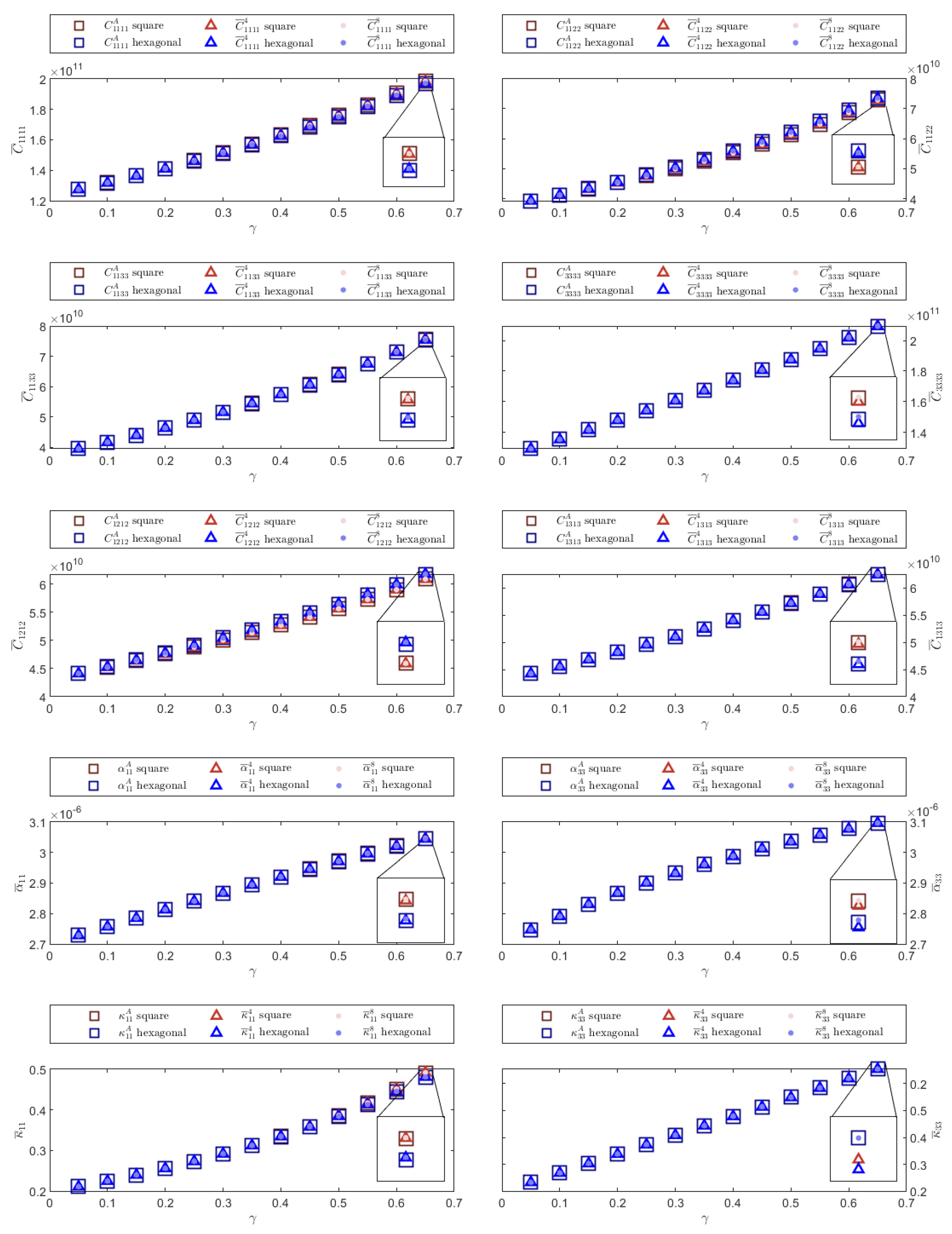
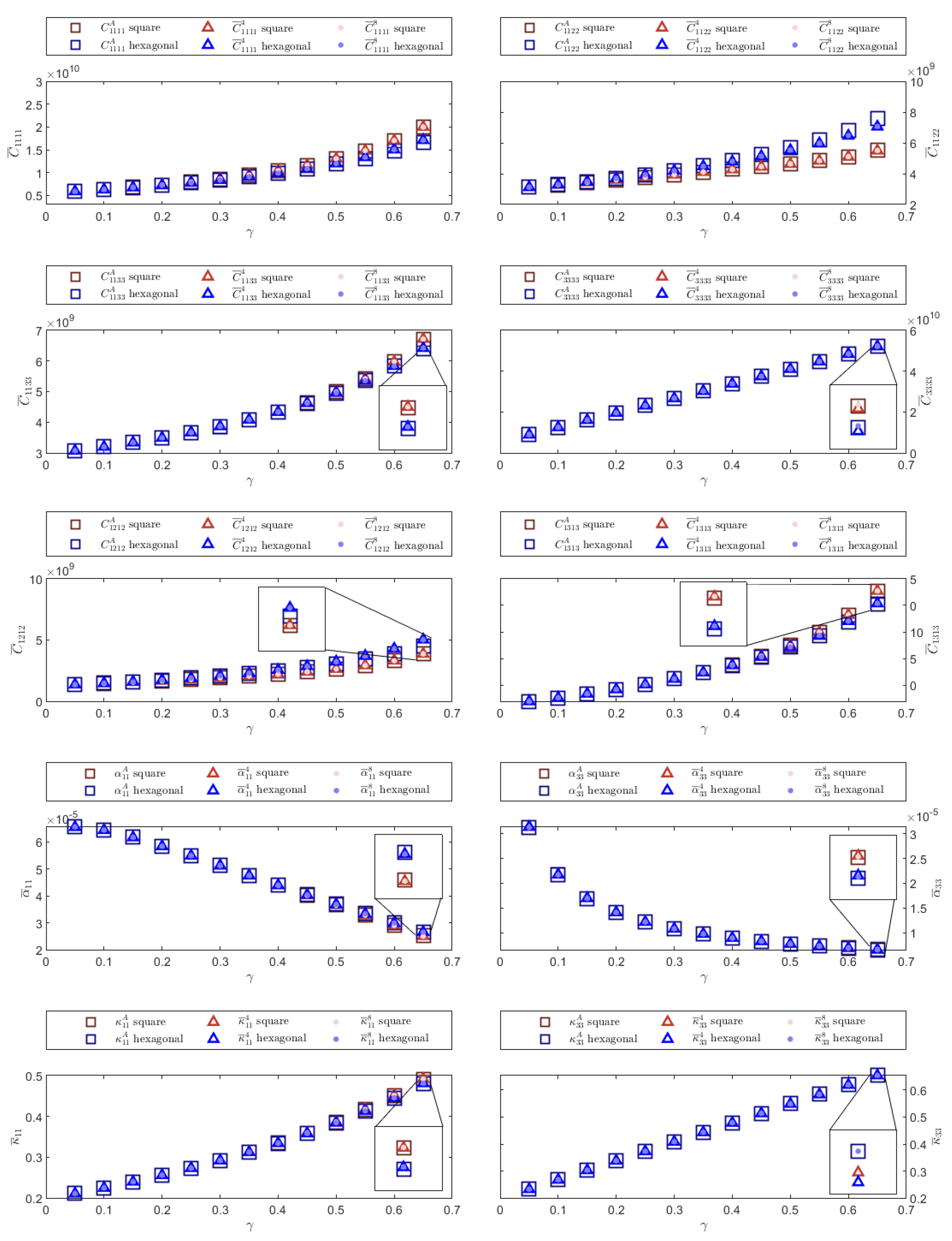
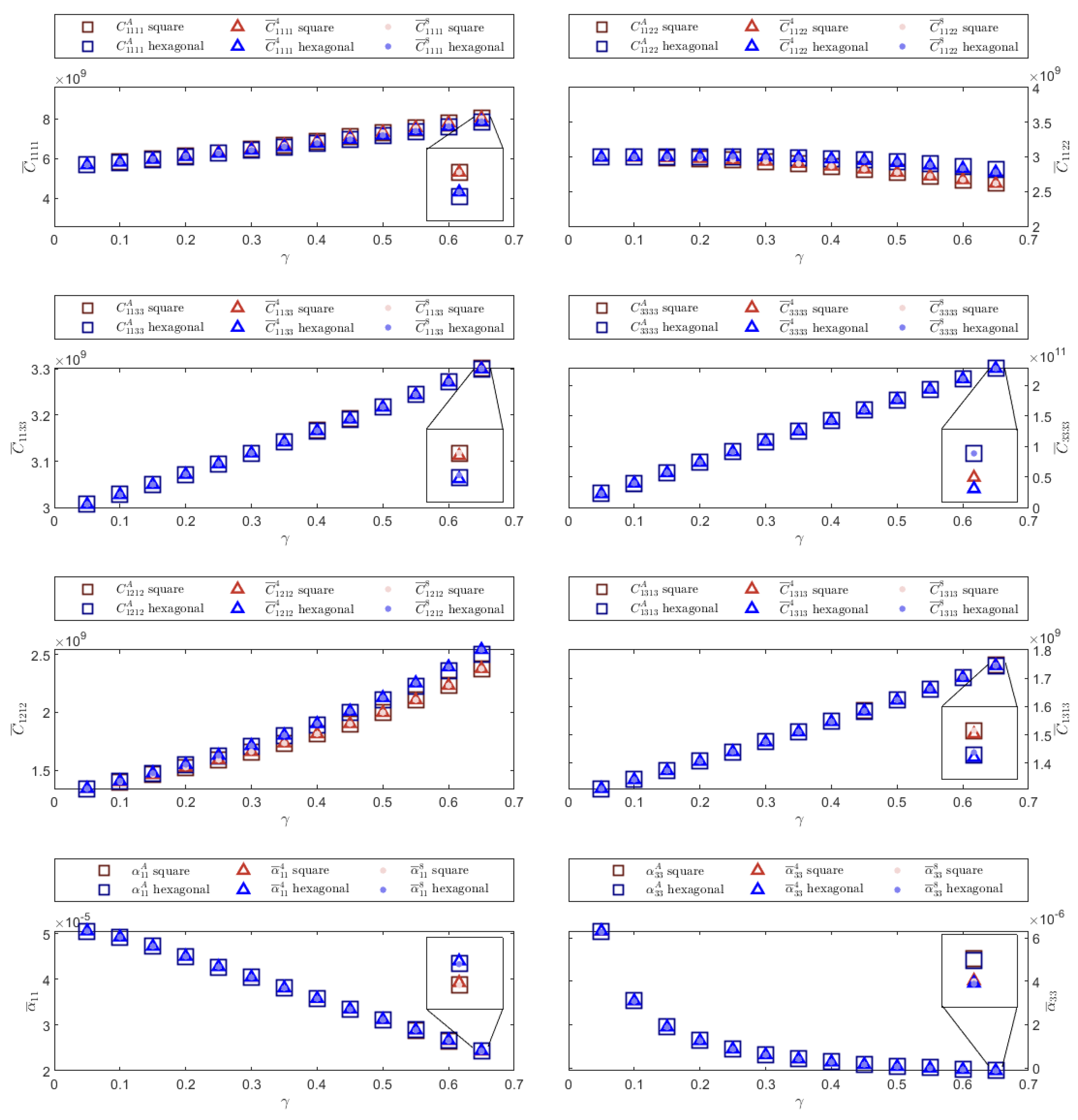
The calculated thermoelastic effective properties are illustrated in this section. In each figure, the effective coefficients obtained by using the linear and quadratic implementations of the FEM for the square and hexagonal fiber distributions are compared. Results calculated for the square and hexagonal cells are shown in blue and red with different intensities, respectively. The values of the effective coefficients determined through the semi-analytical formulas, those calculated by using the linear FEM implementation and those obtained through the quadratic FEM formulation are shown with a square, a triangle and a point, respectively. The superscripts A, 4 and 8 in the legend correspond to the values of the semi-analytical expressions, and those obtained through the linear and quadratic FEM formulations, respectively.

In general, Figure 4, Figure 5 and Figure 6 show that the effective coefficients obtained using both FEM implementations are close to the semi-analytical values. Furthermore, it can be seen that the values calculated by means of the quadratic FEM formulation are closer to the semi-analytical values than those obtained by using the linear FEM formulation. Additionally, some figures show an inset with a smaller scale to show relative differences between the semi-analytic and numerical solutions. Finally, the results obtained when performing the calculations using the square and hexagonal distributions are very similar. Due to the symmetry of the tensors and the periodic cell geometry, there are effective coefficients that yield the same results. Only effective coefficients that have different values are illustrated. Additionally, supplementary data have been included in ref. [32].

The first numerical experiment corresponds to a Nicalon/BMAS composite material. Calculated effective properties for different fiber volume fraction values $\gamma$ are shown. As illustrated in Figure 4, semi-analytical expressions and both FEM implementations provide similar results. The results obtained for the square and hexagonal cell distributions are also similar, differing slightly for large volume fraction values.

From the computed elastic coefficients, it is possible to calculate the effective Young’s modulus and the effective Poisson’s ratio.

Table 4. Young’s modulus ($E^4$) and Poisson’s ratio (${\nu }^4$) for the Nicalon/BMAS composite material calculated by using the linear FEM approximation and those reported in [23].

$\mathit{\gamma }$	E	${\mathit{E}}^4$	$\mathit{\nu }$	${\mathit{\nu }}^4$
	(GPa)	(GPa)
0	$106.00$	$106.00$	$0.233$	$0.233$
$0.2$	$124.89$	$124.86$	$0.248$	$0.248$
$0.4$	$143.74$	$143.71$	$0.263$	$0.263$
$0.6$	$162.53$	$162.50$	$0.276$	$0.276$

shows the effective Young’s modulus ($E^4$) and the effective Poisson’s ratio (${\nu }^4$) values obtained by using the linear FEM approximation and the results reported in ref. [23] (E and $\nu$). As illustrated in Table 4, the estimated values of $E^4$ and ${\nu }^4$ are very similar to those reported in ref. [23].

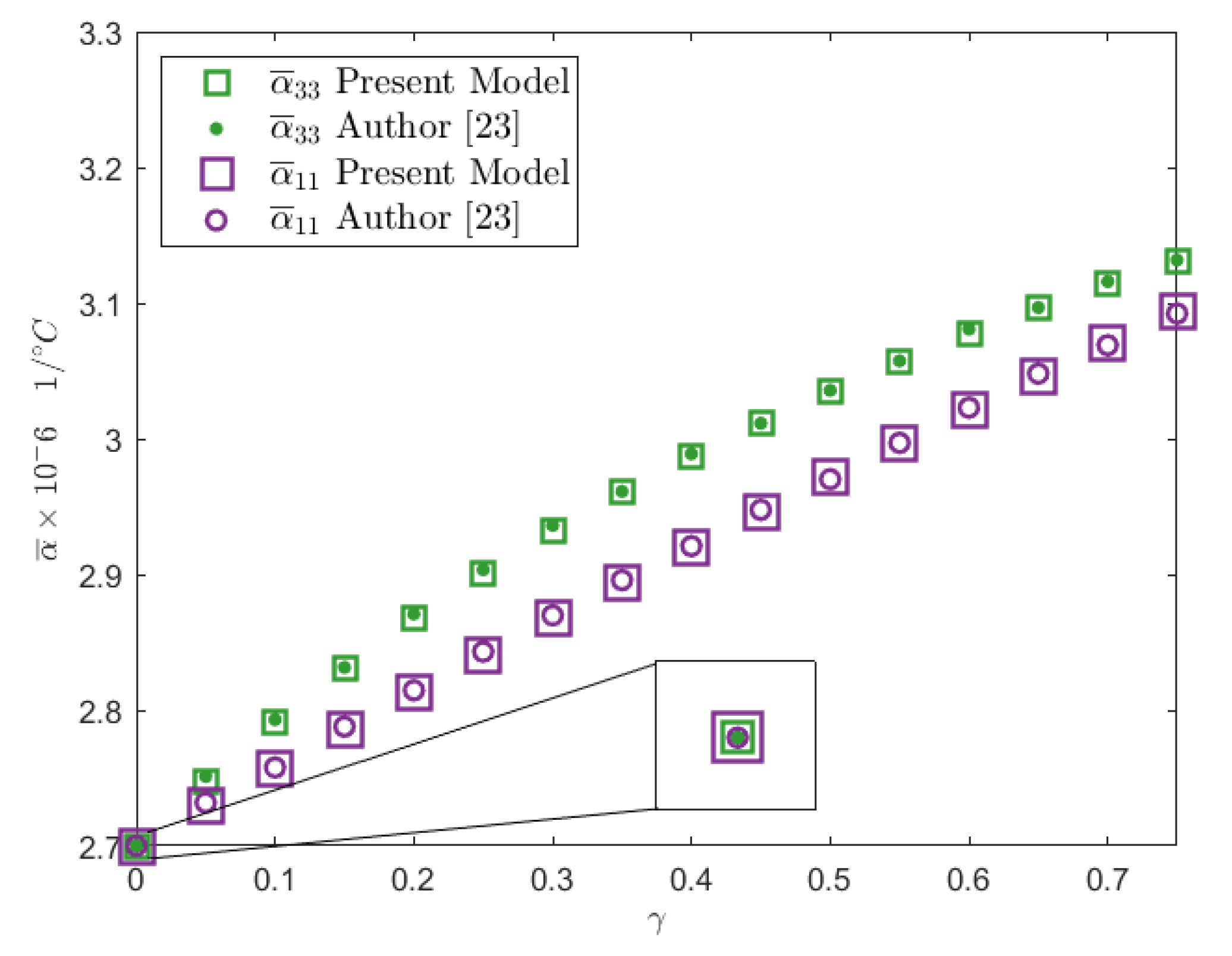
The effective thermal expansion for the Nicalon/BMAS composite material was also calculated in ref. [23] for a square cell distribution. Dots were used in Figure 7 to illustrate the effective thermal expansion coefficients reported in ref. [23]. The results calculated through the linear SAFEM model presented in this work are illustrated with square symbols. The relative difference between the value of ${\overline{\mathit{\alpha }}}_{22}$ and ${\overline{\mathit{\alpha }}}_{11}$ can not be appreciated within the scale shown in Figure 7. Note that for a volume fraction of $\gamma =0$, the effective thermal expansion values correspond to the thermal expansion coefficient of the matrix.

The second example corresponds to the Al-B-Si/Epoxy composite material. This is also an isotropic composite material. Effective elastic properties $\overline{\mathit{C}}$, effective thermal expansion $\overline{\mathit{\alpha }}$ and effective thermal conductivity $\overline{\mathit{\kappa }}$ are illustrated in Figure 5 for square and hexagonal distributions. Calculations for the linear and quadratic FEM approximations, and the semi-analytical expressions are preformed for each coefficient. Results obtained from both FEM implementations are very similar to those estimated when applying the expressions proposed in [8].

The last example belongs to a transversely isotropic composite material formed by Graphite fibers embedded into an Epoxy matrix. Effective thermal properties for Graphite/Epoxy are shown in Figure 6. As in the previous experiments, the values obtained from the quadratic FEM formulation are closer to the semi-analytical values than those obtained by using the linear FEM formulation. In addition, the figure illustrates that there is little variation between the results obtained when performing the calculations using the square and hexagonal distributions.

From the calculated effective coefficients, it is possible to find the effective Young’s modulus and Poisson’s ratio. The linear FEM approximation was used to compute the effective $E_a^4$ and ${\nu }_{31}^4$ values. In

Table 5. Young’s modulus ($E_a^4$) and Poisson’s ratio (${\nu }_{31}^4$) for the Graphite/Epoxy composite material calculated by using the linear FEM approximation and those reported in [23].

$\mathit{\gamma }$	${\mathit{E}}_{\mathit{a}}$	${\mathit{E}}_{\mathit{a}}^4$	${\mathit{\nu }}_{31}$	${\mathit{\nu }}_{31}^4$
0	$3.46$	$3.46$	$0.350$	$0.350$
$0.2$	$71.78$	$71.66$	$0.318$	$0.337$
$0.4$	$140.12$	$139.97$	$0.287$	$0.325$
$0.5$	$208.41$	$208.28$	$0.257$	$0.313$

, the $E_a^4$ and ${\nu }_{31}^4$ values are compared with those given in ref. [23] ($E_a$ and ${\nu }_{31}$).

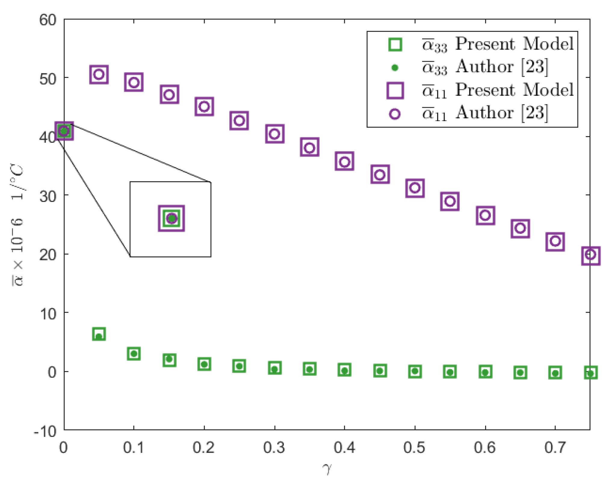
The effective thermal expansion coefficients values for the Graphite/Epoxy composite material have been reported in ref. [23]. Figure 8 shows a comparison between the calculated values of $\overline{\mathit{\alpha }}$ by using the 4-node FEM implementation (square marks) and those reported in ref. [23] (dot marks). Note that if the material is constituted by a pure matrix material, the effective thermal expansion values correspond to the thermal expansion coefficient of the matrix.

5. Elliptical Fiber Cross Section

In this section, the thermoelastic effective coefficients are calculated for a composite material formed by fibers with an elliptical cross section embedded into a matrix with a square distribution as illustrated in Figure 9a. Figure 9b shows the periodic cell Y for the material described and the quarter of the periodic cell is indicated with dashed lines. The ellipse is defined by the length of its semi-axes, denoted by a and b in Figure 9b. It is possible to calculate the volume fraction occupied by the fiber using the following relation $\gamma =ab\pi .$

The isotropic compound formed by Nicalon fibers in a BMAS matrix was used to perform the calculations. The values of the elastic and thermal properties of the fiber and the matrix are listed in Table 2. The values summarized in the following tables show the results calculated through the model presented in this work. The first column shown in each table corresponds to the values of the fiber volume fraction ($\gamma$) used during the numerical simulations. The results obtained by applying the linear and quadratic FEM are shown for each effective coefficient.

Table 6. Calculated effective elastic coefficients for the Nicalon/BMAS composite material formed by elliptical cross-section fibers.

$\mathit{\gamma }$	${\overline{\mathit{C}}}_{1111}^4\times {10}^{11}$	${\overline{\mathit{C}}}_{1111}^8\times {10}^{11}$	${\overline{\mathit{C}}}_{2222}^4\times {10}^{11}$	${\overline{\mathit{C}}}_{2222}^8\times {10}^{11}$	${\overline{\mathit{C}}}_{3333}^4\times {10}^{11}$	${\overline{\mathit{C}}}_{3333}^8\times {10}^{11}$
$0.05$	$1.27960955$	$1.27973266$	$1.27194469$	$1.27207959$	$1.29390269$	$1.29422463$
$0.20$	$1.43614638$	$1.43635433$	$1.39674836$	$1.39689302$	$1.47963878$	$1.47998033$
$0.35$	$1.63682994$	$1.63725000$	$1.53507473$	$1.53525178$	$1.67513306$	$1.67554036$
$\mathbf{\gamma }$	${\overline{\mathit{C}}}_{\mathbf{1122}}^{\mathbf{4}}\times {\mathbf{10}}^{\mathbf{10}}$	${\overline{\mathit{C}}}_{\mathbf{1122}}^{\mathbf{8}}\times {\mathbf{10}}^{\mathbf{10}}$	${\overline{\mathit{C}}}_{\mathbf{1133}}^{\mathbf{4}}\times {\mathbf{10}}^{\mathbf{10}}$	${\overline{\mathit{C}}}_{\mathbf{1133}}^{\mathbf{8}}\times {\mathbf{10}}^{\mathbf{10}}$	${\overline{\mathit{C}}}_{\mathbf{2233}}^{\mathbf{4}}\times {\mathbf{10}}^{\mathbf{10}}$	${\overline{\mathit{C}}}_{\mathbf{2233}}^{\mathbf{8}}\times {\mathbf{10}}^{\mathbf{10}}$
$0.05$	$3.92304771$	$3.92354793$	$3.96130051$	$3.96190070$	$3.93459920$	$3.93537033$
$0.20$	$4.52908131$	$4.52992368$	$4.71404476$	$4.71505763$	$4.57737822$	$4.57825998$
$0.35$	$5.25352632$	$5.25513429$	$5.66087808$	$5.66289169$	$5.30810165$	$5.30930182$
$\mathbf{\gamma }$	${\overline{\mathit{C}}}_{\mathbf{2323}}^{\mathbf{4}}\times {\mathbf{10}}^{\mathbf{10}}$	${\overline{\mathit{C}}}_{\mathbf{2323}}^{\mathbf{8}}\times {\mathbf{10}}^{\mathbf{10}}$	${\overline{\mathit{C}}}_{\mathbf{1212}}^{\mathbf{4}}\times {\mathbf{10}}^{\mathbf{10}}$	${\overline{\mathit{C}}}_{\mathbf{1212}}^{\mathbf{8}}\times {\mathbf{10}}^{\mathbf{10}}$	${\overline{\mathit{C}}}_{\mathbf{1313}}^{\mathbf{4}}\times {\mathbf{10}}^{\mathbf{10}}$	${\overline{\mathit{C}}}_{\mathbf{1313}}^{\mathbf{8}}\times {\mathbf{10}}^{\mathbf{10}}$
$0.05$	$4.41223185$	$4.41272590$	$4.40911237$	$4.40937696$	$4.43618802$	$4.43675684$
$0.20$	$4.76524287$	$4.76572697$	$4.74674572$	$4.74701946$	$4.87931685$	$4.88007469$
$0.35$	$5.13161355$	$5.13213498$	$5.10948217$	$5.10996326$	$5.40108898$	$5.40233224$

shows the elastic effective coefficients calculated by using linear and quadratic FEM approximations for different values of $\gamma$. The calculations were performed using an aspect ratio for the ellipse of $\raisebox{1ex}{$a$}\!\left/ \!\raisebox{-1ex}{$b$}\right.=2$. Finally, the differences between the different approximations used in this work are shown in each table.

Table 7. Calculated effective thermal coefficients ($\overline{\mathit{\alpha }}$ and $\overline{\mathit{\kappa }}$) for the Nicalon/BMAS composite material with elliptical cross-section fibers.

$\mathit{\gamma }$	${\overline{\mathit{\alpha }}}_{11}^4\times {10}^{-6}$	${\overline{\mathit{\alpha }}}_{11}^8\times {10}^{-6}$	${\overline{\mathit{\alpha }}}_{22}^4\times {10}^{-6}$	${\overline{\mathit{\alpha }}}_{22}^8\times {10}^{-6}$	${\overline{\mathit{\alpha }}}_{33}^4\times {10}^{-6}$	${\overline{\mathit{\alpha }}}_{33}^8\times {10}^{-6}$
$0.05$	$2.73385948$	$2.73390018$	$2.72449162$	$2.72459329$	$2.74760277$	$2.74783932$
$0.20$	$2.83418424$	$2.83428939$	$2.79542871$	$2.79550615$	$2.86780699$	$2.86799415$
$0.35$	$2.93802973$	$2.93824187$	$2.85826937$	$2.85832620$	$2.96185289$	$2.96202121$
$\mathbf{\gamma }$	${\overline{\mathbf{\kappa }}}_{\mathbf{11}}^{\mathbf{4}}$	${\overline{\mathbf{\kappa }}}_{\mathbf{11}}^{\mathbf{8}}$	${\overline{\mathbf{\kappa }}}_{\mathbf{22}}^{\mathbf{4}}$	${\overline{\mathbf{\kappa }}}_{\mathbf{22}}^{\mathbf{8}}$	${\overline{\mathbf{\kappa }}}_{\mathbf{33}}^{\mathbf{4}}$	${\overline{\mathbf{\kappa }}}_{\mathbf{33}}^{\mathbf{8}}$
$0.05$	$0.21481147$	$0.21479529$	$0.20868715$	$0.20870690$	$0.23288928$	$0.23309971$
$0.20$	$0.27719544$	$0.27724200$	$0.24382996$	$0.24384613$	$0.33818843$	$0.33839992$
$0.35$	$0.38081376$	$0.38114152$	$0.28217703$	$0.28219913$	$0.44347312$	$0.44369995$

shows the calculated values of the thermal effective coefficients (thermal expansion and thermal conductivity) for the Nicalon/BMAS composite material formed by elliptical fibers. Additionally, the difference between FEM approximations are also illustrated. On the one hand, composites with circular cross-section fibers have the same values for the effective coefficients ${\overline{C}}_{2323}$ and ${\overline{C}}_{1313}$. On the other hand, when the composite material is made with elliptical cross-section fibers, ${\overline{C}}_{2323}$ and ${\overline{C}}_{1313}$ do not have the same value. Similarly, the thermal expansion coefficients ${\overline{\mathit{\alpha }}}_{11}$ and ${\overline{\mathit{\alpha }}}_{22}$ and thermal conductivity coefficients ${\overline{\mathit{\kappa }}}_{11}$ and ${\overline{\mathit{\kappa }}}_{22}$ have the same values for composites with circular cross-section fibers and different values for composites with elliptical cross-section fibers, as observed in Table 6 and Table 7. The aforementioned difference between effective coefficients is expected because the fiber is not evenly distributed in the $y_1$ and $y_2$ directions.

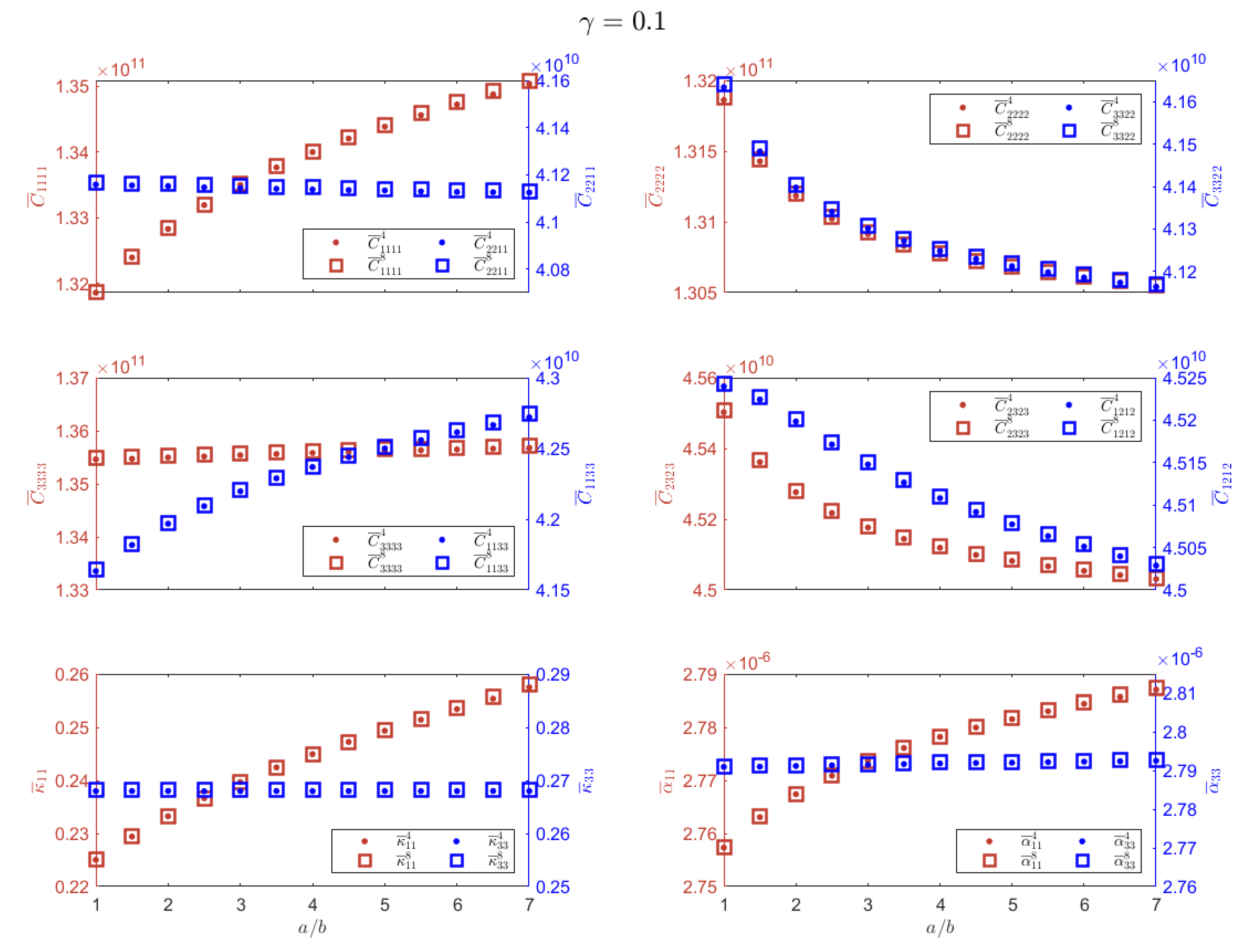
To study the effects of the fiber geometry on the values of the effective properties, several experiments were performed. The fiber volume fraction value $\gamma =0.1$ was kept constant, and the aspect ratio of the fiber was changed. The shape of the fiber varied by considering zero eccentricity values where $\raisebox{1ex}{$a$}\!\left/ \!\raisebox{-1ex}{$b$}\right.=1$ to large eccentricity values where $\raisebox{1ex}{$a$}\!\left/ \!\raisebox{-1ex}{$b$}\right.=7$. Figure 10 shows the effective thermoelastic properties calculated through both FEM implementations: linear and quadratic. Linear values are shown using dots and quadratic values are illustrated using square symbols. Each subfigure represents two different effective coefficients.

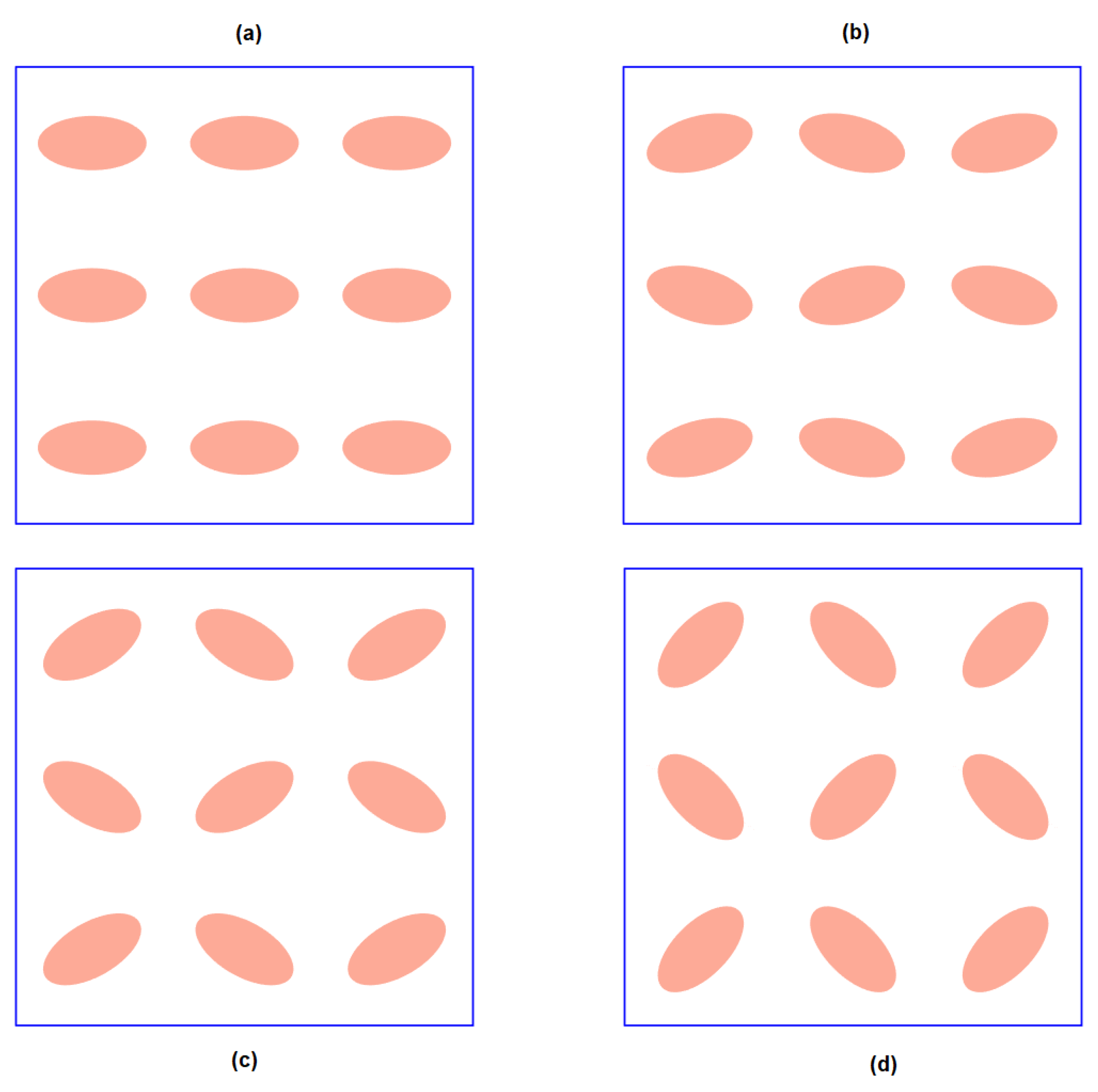
Distributions of the Fiber’s Cross Section with Different Orientations

In this section, the effect of the elliptical cross-section orientation on the effective thermoelastic properties is analyzed. The calculated results of the effective coefficients are closely related to the fiber geometry, as mentioned in the previous section. For the elliptical cross section, it has been shown that ${\overline{C}}_{2323}$ and ${\overline{C}}_{1313}$, and ${\overline{\mathit{\kappa }}}_{11}$ and ${\overline{\mathit{\kappa }}}_{22}$, do not have the same values. Square periodic cells composed of thirty-six ellipses were considered to estimate the relation between the effective properties of the composite material and the orientation of the elliptical fibers. Consequently, the cell quarter must have a square with nine ellipses, as shown in Figure 11.

The effect of having fibers with different orientations is determined by the rotation of the fiber’s cross section with respect to the $y_3$ axis. Different fiber orientations ($\theta =0^{\circ },5^{\circ },{10}^{\circ },{15}^{\circ },{20}^{\circ },{25}^{\circ },$${30}^{\circ },{35}^{\circ },{40}^{\circ }$ and ${45}^{\circ }$) were considered, where $\theta =0^{\circ }$ indicates an equally aligned fiber distribution, as shown in Figure 11a. Figure 11d illustrates the $\theta ={45}^{\circ }$ orientation.

Effective thermoelastic properties were calculated using an aspect ratio of $\raisebox{1ex}{$a$}\!\left/ \!\raisebox{-1ex}{$b$}\right.=2$ and $\gamma =0.2$. Figure 12a shows the effective coefficient values ${\overline{C}}_{1313}$ and ${\overline{C}}_{2323}$ for different orientations $\theta$. The effective coefficient ${\overline{C}}_{1313}$(${\overline{C}}_{2323}$) increases (decreases) monotonically as a function of $\theta$ until ${\overline{C}}_{1313}$ has the exact same value as ${\overline{C}}_{2323}$ for $\theta ={45}^{\circ }$, where the composite material shows a transversely isotropic behavior as illustrated in Figure 12a. The thermal conductivity coefficients ${\overline{\mathit{\kappa }}}_{11}$ and ${\overline{\mathit{\kappa }}}_{22}$ show a similar monotonic behavior as a function of $\theta$, reaching the expected transversely isotropic behavior for $\theta ={45}^{\circ }$, as observed in Figure 12b.

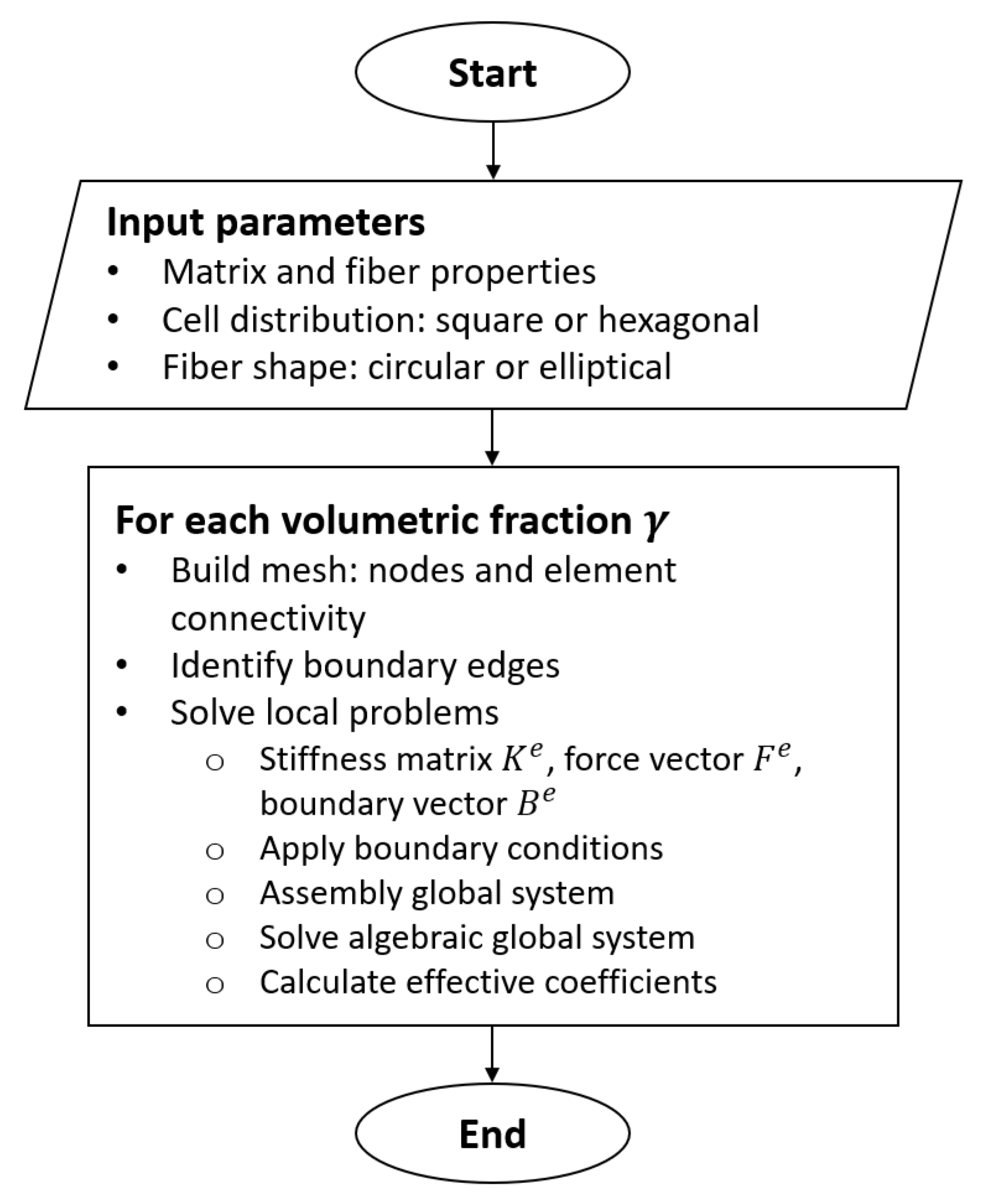
6. Computational Implementation

A MATLAB program was developed to calculate the thermoelastic effective coefficients by using square or hexagonal cell distributions. Since the representative cell has symmetric geometry, calculations are performed by using only $\raisebox{1ex}{$1$}\!\left/ \!\raisebox{-1ex}{$4$}\right.$ of the cell. This allows to reduce the number of operations and CPU time.

The program receives as input the type of cell that constitutes the composite material as well as the elastic (Young’s modulus, Poisson’s ratio) and thermal properties (conductivity and thermal expansion) of the materials that correspond to the fiber and the matrix. The fiber volume fraction values $\gamma$, for which the calculations of the effective properties will be performed, are selected. For each value of $\gamma$ a mesh that discretizes the quarter of the cell is generated. The method described in ref. [30] was used to construct an 8-node quadrilateral mesh. The 4-node quadrilateral meshes are created by using the obtained 8-node quadrilateral meshes. The effective thermoelastic properties, such as the elastic coefficients $\overline{\mathit{C}}$, the thermal expansion $\overline{\mathit{\alpha }}$ and thermal conductivity $\overline{\mathit{\kappa }}$ coefficients, are obtained for each value of $\gamma$. Linear and quadratic FEM formulations are used to solve the local problems obtained from the AHM. The generated meshes are used to perform calculations through the linear and quadractic FEM formulations, respectively. Graphics are created and tables are estimated for each value of $\gamma$, where the numerical values of the thermoelastic effective coefficients are shown.

As a result of applying the AHM and in order to obtain the thermoelastic effective coefficients, the local problems must be solved for each value of $\gamma$. The values of $\gamma$ vary from 0 to 1 with a step size of $0.05$ as a default value. For each local problem, every element within the mesh is analyzed. The local matrices of each element are calculated and the global matrices are assembled. The dimension of the matrices is twice the number of nodes in the mesh, for the elastic plane local problems and the ${}_{pp}T$ local problem. The dimension of the matrices is the same as the number of nodes in the mesh, for the elastic anti-plane local problems and the ${}_{q}I$ local problems. The matrices have several zero values, and due to the large volume of calculations that must be performed with large matrices where a large number of zeros is present, the MATLAB’s sparse data structure was used. The sparse data structure stores only the positions and the values of the elements that are not zero, occupying a significantly less amount of memory. Additionally, MATLAB redefines the sparse array operations so that only nonzero elements are considered. Finally, approximately $30\%$ of the execution time can be saved through this strategy.

Figure 13 shows a flowchart that describes the computational implementation steps.

7. Conclusions

The generalization of the SAFEM for thermoelastic composite materials formed by elliptical cross-section fibers with perfect contact between the interface and the matrix was proposed. Square and hexagonal cell distributions were considered. Effective properties were obtained for three different composite materials. The calculated results by using the linear and quadratic FEM formulations are very similar to the semi-analytical values reported by other authors. Additionally, the calculated effective properties for the square and hexagonal distributions are very similar. The effective coefficients for a composite material with several orientations for an elliptic cross section fiber show a non-isotropic behavior according to the results of this work. Additionally, as the angle of orientation increases, the behavior of the composite material approaches smoothly to a transversely isotropic behavior.