Abstract
The standard problem of engineering geophysics, solved for road and house building and other construction types, is in the localization of areas with increased mobility in the upper part of a geological cross-section and in the parameterization of this mobility in terms of seismic intensity. There is a standard approach, according to which researchers assess the elastic strength characteristics of the core to a depth of about 30 m, implement the accumulation of seismogram observations, simulate accelerograms for particular conditions and, taking into account the data of complex geophysical methods, calculate the increment of seismic intensity as one of the parameters of a seismic hazard. The final result of this approach has the form of a seismogenic hazard map and a set of recommendations including the consideration of identified areas with a significant increasing seismic intensity increment, due to the peculiarities of the geological structure of polygons. This result is reliable, but very expensive, and requires the development of primary estimations of the rock massif with reduced resistance to external loads, which would optimize the efforts in engineering drilling and in field geophysical measurements in order to densify their spatial grid in the vicinity of a priori known positions with an increased seismogenic hazard. In addition, relatively sparse grids of wells, as well as local geophysical profiles laid under conditions of a complicated landscape, do not accurately localize risky areas in order to focus the attention of builders on strengthening the specific part of raised constructions. Following the wishes of our customers and relying on long-term testing of our interpretational developments, we formed an approach to primary hazard forecasting based on remote sensing data and digital elevation models, which can be classified as data with relatively free access. This article presents the results of research which was based on these free-of-charge data and which was developed in the field of construction of ground engineering structures for agricultural purposes, where one of the factors of mobility in the upper part of a cross-section is intensive karstification. Basically, the construction area according to the general seismic zoning maps is seismologically passive, though the relatively fast dynamics of karst determines the relevance of the detailed seismic zoning. The results of our interpretations are verified by deep geological and structural reconstructions based on wave analogies. The representativeness of the final forecast was confirmed by subsequent seismic assessments, which is related to the scientific novelty of the presented article. The authors’ technology for the qualitative and quantitative interpretation of remote sensing data and digital elevation models with high resolution provides the opportunity to increase the spatial resolution of seismic microzonation forecasts, implemented by standard geophysical methods, and it determines the practical significance of completed research.
1. Introduction
Strictly speaking, the problem, which we solve, has a narrow engineering nature; it is reduced to parametric mapping of the elements of fracture tectonics and their ranking. Nevertheless, linking our work to the general research cycle, we involuntarily touch upon a wide-ranging area of engineering and geological surveys associated with the assessment of primary (endogenous) and secondary seismicity. Without departing from the essence of our work, we should note that these assessments are traditionally divided into the macroseismic method and seismic microzonation. The basis of macroseismic assessments is formed by small-scale maps of a general seismic hazard, specified on the basis of systematic seismological observations, updating the geological maps and population survey. In general, the structure of maps of a macroseismic (regional seismic) hazard is determined by active continental margins, young folded structures and the position of regional suture zones. The development of macroseismic assessments has been systematically implemented since the 1960s; it is associated, first of all, with the publications by American geophysicists (B. Bender (1972), C.A. Cornell (1968), etc.), through whose efforts the first versions of computer programs for seismic hazard calculation were developed. From the other side, in the USSR and Russian Federation, seismic hazard assessments had a systematic, methodological and physico-mathematical character too; this way of research is associated with V.I. Ulomov. (1999), S.V. Medvedev (1960) and others. Seismic microzonation is based on macroseismic determinations and parametrically takes into account the influence of soil conditions on seismic activity in the form of integral parameters of the seismic intensity increment. This increment has the form of correction to the initial seismic intensity, determined at the stage of macroseismic studies; this correction is varied in the range from −1 to +1 and calculated taking into account the set of geological and structural factors. In most countries, seismic microzonation is carried out in the parameters of seismic ground motions, which can be used immediately for further engineering computations [1,2]. In the Russian Federation, this microzonation is traditionally performed in units of intensity with accompanying assessments of resonance frequencies and simulation of ground vibration accelerograms [3,4]. In addition to obvious geological and geodynamic anomalies that determine the growth of a seismic hazard, the processes and objects affecting the growth of the seismic intensity increment include areas of intense gradient in the heights of the Earth’s relief, shallow depths of the groundwater table and significant dynamics of exogenous processes (karst and gully formation). The genetic relationship between geological and geodynamic anomalies, as well as the mentioned objects and processes, on the one hand, and the elements of fracture tectonics that form geodynamic zones, on the other hand, is apparent.
The idea of mapping geodynamic zones in the form of extended geostructural elements based on the analysis of remote sensing images is tested when compiling general seismic hazard maps for different probabilities of a seismogenic event [5]. However, the use of the distance basis in this case requires some additional level of a priori information concerning the position and intensity of seismogenic disturbances relative to the geodynamic zone, as well as the characteristics of the geodynamic zone itself (fracture width, surface fracture length, etc.). Such assessments are feasible on a regional scale, while with the transition to detailed seismic zoning and further to seismic microzoning, the level of a priori information required for representative conclusions on the detailing of seismogenic hazardous zones noticeably increases. Considering the high cost of field work, which determines this level of a priori information, we can talk about a natural tendency to assess the seismic hazard based on a family of indirect signs related to individual engineering structures [6]. At the stage when these structures are only being planned, attempts to find a correlation between the characteristics of the landscape observed in remote sensing images and the characteristics of seismicity recorded in some databases can be called obvious. The methodological basis for detecting this correlation is rather modest, since it relies on particular cases of landscape anomalies and does not contain a fundamental concept. For example, the method of localizing seismogenic hazardous areas based on mapping the lineament density maxima [7] can be called quite popular. As another example, we can point to the study of the empirical relationship of individual faults, manifested in the system of lineament structures on remote sensing images, on the one hand, and earthquake epicenters, on the other hand [8]. There is an interesting work on the assessment of the variability of the directional rose of lineaments under conditions of high-intensity seismogenic disturbances [9]. Summarizing publications and works similar to this, it can be argued that there is a direct functional relationship between the characteristics of seismicity and the characteristics of landscape variability: our earlier work confirms this [10] and allows us to apply quantitative estimates of this variability in a systemic form in this study.
At the initial stages of geophysical engineering and ecological engineering support of (road and house) building, when the known data are limited only by coordinates of the area of interests, reliable mapping of geodynamic zones and their quantitative parameterization using free-of-charge data can form the essence of the primary forecast of seismically hazardous areas for their subsequent verification with standard and more expensive approaches. Actually, the processing of remote sensing data and digital elevation models in engineering problems is the standard work for geomorphologists. The advantage of our approach in comparison to classical decoding of remote sensing data is in using quantitative and quantitative interpretation, similar to assessments applied in geophysics, while geomorphology operates with empirical classifications and visual expert estimations.
Turning to the choice of area of interest, one can note from the point of view of macroseismic assessment and seismic microzonation that this area was not anything remarkable. It was a commonplace district with a relatively smoothed relief of the Earth’s surface, intended for construction of greenhouses and located far from any significant endogenous seismic manifestations—in the central part of ancient Russian plate, in the north of the Central Russian Upland. Thus, the requirements of regulatory documents for geophysical engineering support of building would be purely formal ones, if one does not take into account the peculiarities of geological structures both at small-scale and large-scale levels. The investigated area is located on the joint of two structures—the northern slope of the Voronezh massif and the southern slope of the Moscow depression (Central Russian syneclise). In addition, it is mapped within the periphery of a large circular geological structure being 250 km in diameter. This circular structure is observed in the territory of the Tula and Oryol regions (Tula dome-ring structure) and coincides with a significant part of Central Russian Upland (Figure 1a) [11]. Hypothetically, dome-shaped formations are the result of generation of a hot spot or, in other words, the impact of endogenous plumes. On the Earth’s surface, similar vertical motion of plumes is often correlated with elevations, and along their periphery, they are limited by ring and concentric faults, including deep ones. These processes are complicated by the formation of a set of different order linear tectonic faults, which form, in particular, a fairly branched network in the Tula region. The most famous of them is the regional linear fracture with a latitudinal direction, crossing through the entire Oka basin [12], which includes the settlements Tula and Shchekino (Figure 1b). There are few kilometers from Shchekino to the area of planned construction. In the eastern part of the Tula region, there is one more regional fault with a northeastern direction—it is propagated approximately along the line of cities of Efremov, Uzlovaya, Novomoskovsk and Venev, i.e., it is placed approximately 35–40 km from the object of investigation. This fault probably originates from the Mediterranean coast and is traced to the territory of the Russian Federation in the northeastern direction up to the Yamal Peninsula.
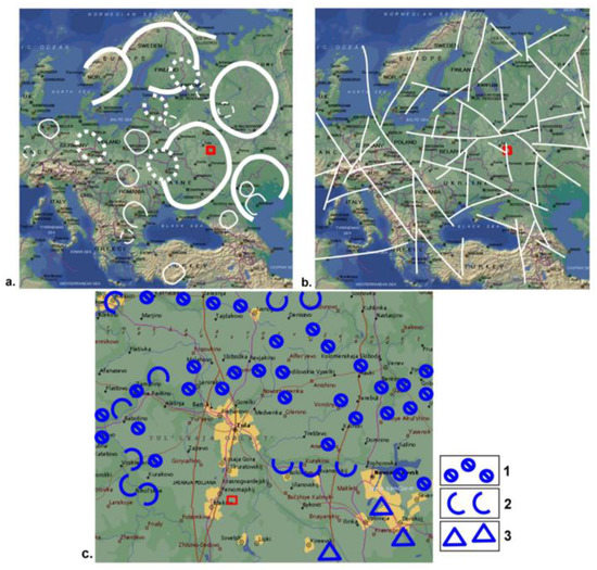
Figure 1.
Geostructural position of investigated area (according to Brykhanov V.N., Boosh V.A., Chikishev A.G.): (a) schematic map of regional circular formations of the 1st–4th orders within the contact of the East European Platform, West European Plate and Mediterranean belt; (b) schematic map of regional lineaments in the area of this contact. The approximate position of the estimated territory is marked by the red line; (c) the fragment of the regional map of geophysical engineering zoning of the Tula region and adjacent territories (according to Popov [13]) (1—karst, 2—landslide phenomena, 3—areas of development of subsidence processes; area of interest is located slightly south with regard to the Tula, where the processes of karst formation and vertical subsidence in the upper part of the geological cross-section are also observed). One can see the area of interest has an anomalous position: at the regional scale—within a relic hot spot and on the intersection of geodynamic zones; at a large scale—in the vicinity of the river which is characterized by intensive landslide and karst formation.
Despite the location of the Tula region being in the zone of low-intensity seismic responses and rather far from the epicenters of earthquakes registered in the Alpine belt, the seismic activity is not negligible here. This is indirectly indicated by the morphology of the map of general seismic zoning (2015-C: the period of shaking is around 5000 years with a 1% probability of exceeding the calculated seismic intensity within 50 years) [14,15,16]. Although, in the vicinity of the investigated object, this map has a monotonic and low-intensity structure, there is a gradient zone from scores 5 to 6–7 of the Richter scale at the distance of about 130–140 km. Seeing the strike of anomalous seismic zones in sublatitudinal or northeastern directions, one can suppose their genetic relationship with the regional disjunctives mentioned above.
The vertical cross-section of the region [17] is characterized by monoclinal bedding of structural and compositional complexes with nonconformity at the contact of the Vendian, Archean-Proterozoic formations and Devonian deposits. In the relief of contacts of the stratified mining massif, the synform and Vendian layer thinning in the vicinity of investigated area can be observed. This feature of the geological structure is supposed to be the marker of the presence of regional deep faults which directly cross the estimated territory and are inherited by structural anomalies. Moving up through the cross-section, thick Devonian deposits as well as Carboniferous formations can be noted, including widespread limestones, which caused karst formation and, as the result, the danger of vertical subsidence during interaction of near-surface structural and compositional complexes with elements of fracture tectonics.
Karst phenomena observed north and south of Tula city [18,19,20,21] are mainly caused by interaction between groundwater and Mississippian limestones as well as Devonian gypsum (Figure 1c). The karst in Upper Devonian gypsum is especially intense. In the investigation region, the karst is observed in various forms: sinkholes, hollows, gullies, karst lakes, disappearing rivers, coastal depressions, karst depressions, niches and underground voids. The intensity of karst development is estimated by the area of its manifestation and by the specific volume of mapped karst cavities. This intensity is higher in the Tula region in comparison with the neighboring territories—this is due to the greater fragmentation and relatively high fracturing of carbonate strata. The dependence of karst formation both on dynamics of endogenous fracture tectonics and on exogenous factors [13,22,23] leads to continuous dynamics of karst development and to a nonzero hazard of the new vertical subsidence under the fast healing of karst formations. This implies the relevance of geodynamic evaluation of the area [20,24,25], especially under conditions of extensive mine workings, which are observed within the investigated object. Previously, the authors carried out the investigation of a seismogenic hazard in the vicinity of geodynamically active geoblocks because of activation of fault tectonics under conditions of hydraulic fracturing [10], with application of non-potential geofields. This article presents the extension of a systematic approach to the analysis of these geofields within Earth’s geodynamically stable crust.
2. Data and Methods
The key element of the database is remote sensing data combined with digital models of the Earth’s surface elevations, including, in particular, aerophotos and satellite images of the terrain. At the middle scale (1:50,000–1:100,000), remote sensing data were downloaded from open access USGS website EarthExplorer; at the large scale, remote sensing images were produced by an unmanned aerial vehicle survey based on the GeoScan technology. A detailed digital elevation model was developed in two ways: the first one (main) included digitizing originally analogous topographic maps available through a licensed Android application, ATLOGIS Geoinformatics; the second way was used for the mentioned digitizing update—it was based on stereophotography and laser sensing during the unmanned aerial vehicle survey.
Remote sensing data combined with digital elevation models are defined as scaled-down models of the terrain, where geological and structural anomalies are encoded in combinations of landscape components, and these combinations are encoded in the set of half-tone photo anomalies. Geological heterogeneities, which are not explicitly observed at the surface due to masking by soil and vegetation cover, intense weathering processes and anthropogenic influences, are clearly manifested in remote sensing data. Physically, this is explained by the evolutionary process of landscape formation within the considered territory, where all landscape components functionally depend on geological heterogeneities. At the stage of expert decoding [26], the lineament field is reconstructed both with remote sensing data and DME for reliable verification of results. The lineament as a linearized (straightened) landscape element is traced through heterogeneous forms of half-tone anomalies in remote sensing data and heterogeneous forms of relief in order to map the elements of fracture tectonics, obtaining the latest activation [25,27]. Expert decoding is based on visual estimations and manual, little-automated operations with one or the set of most contrasting spectrum bands. Here, the contrast is traditionally defined as parameter
computed by the values of the optical density field between pairs of neighboring objects and averaged over the entire considered area.
Scalar fields of parameters derived from the initial scalar field by means of application of differential operators and estimation of exponential parameters are a hint in monitoring the results of expert decoding. The calculation of shadow forms of the geofield surface , when this surface is illuminated by a homocentric source [28], can be defined as the simplest transform of this type. If is the angle formed by the incident ray and the horizon plane, is the angle between the conditional direction to the north and the projection of the incident ray onto the horizontal plane, counted clockwise, and
is the slope angle of the virtual surface of the geofield, and
is the angular sector of the view, where
is the number of matrix elements composed by values of the geofield in the sliding window:
Then, the shadow forms of the geofield surface are represented by the parameter
Contrasting of the local half-tone structures is implemented by preliminary application of differential operators, for example, the Sobel operator [29,30] used in the convolution mode in the 3 × 3 window with the following transfer functions:
The result of recalculation is assigned to the center of the sliding window.
The left transfer function contrasts the geostructural lines of the sublatitudinal strike, and the right transfer function underlines geostructures of the submeridional strike (Figure 2a,b). Another example is borrowed from thermodynamics (Figure 2c) and reflects the ratio of ordered components of the geofield against disordered (chaotic) components in the structure of the scalar field (Figure 2c) [31,32]:
entropy, where is the probability of the -th state of the physical system (in practice, it is the frequency of realization of the -th state, which is described as the interval of field values between two adjacent isolines).
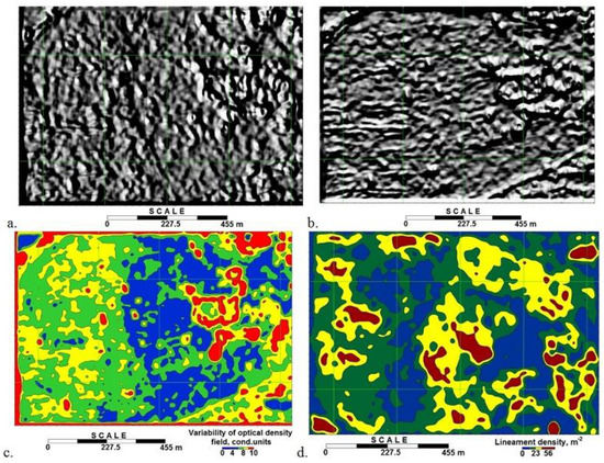
Figure 2.
The example of recalculation of remote sensing data and digital elevation model into a form which clearly demonstrates the position and orientation of linear (geodynamic) zones: (a,b) the result of applying differential operators to digital elevation models for contrasting the positions of geodynamic zones of different strike azimuths (northwest and northeast, respectively); (c) characterization of the degree of disorder (entropy) of the optical density field of the considered area; (d) field of lineaments density (the degree of fragmentation in the upper part of the cross-section) of the survey area (Shchekinsk area, Tula region). One can see the ways of tracing linear geodynamic zones which verifies the results of automated lineament analysis.
The key procedure in the applied system of transforms is developed under this project in automated lineament analysis which accompanies and verifies expert lineament decoding. The algorithm includes searching for extremum points in the system of values of the initial scalar field as well as in the system of values of the calculated field of the horizontal gradient modulus. The next procedure is rotation of elementary lineaments around each of the mentioned points based on a standard rotation matrix and local spline interpolation. The final strike azimuth of a particular lineament is chosen by the criterion of the minimum of the dispersion functional. The result of such recalculation is represented by the set of coaxial structures derived by the generalization procedure. The latter is represented, first of all, by a statistical sorting of one-oriented structures with elimination of quasiperiodic lineament nets. Three standard procedures form the basis of presorting: determination of the direction rose of isolines of the scalar field based on the structure of the autocorrelation function; estimation of variance of strike azimuths of local lineaments; elimination of the set of elementary lineaments with the highest strike azimuth variances. The second component of the generalization procedure includes combining the tips of the nearest coaxial lineaments into macroscopic straightened structures (geostructural lines) with the subsequent smoothing of these structures. The algorithm also includes logical procedures, such as elimination of “blind” intersections of lineament structures of different azimuths as well as elimination of the priority of extended linear elements in comparison with arch concentric elements. The generalization of results of lineament decoding in the form of a map of the lineament density distribution is an important operation for final interpretation. Since the methodological foundations of seismic hazard maps are based on a direct analogy between lineaments and fracture tectonics [14,33], the increasing lineament density can be correctly interpreted as increasing the fragmentation in the upper part of the cross-section. Numerically, the procedure is based on counting the number of tips of selected lineaments per unit area of the integration interval (Figure 2d).
Morphotectonic analysis is an independent operation that verifies the morphostructural reconstructions described above and information about the position of areas of reduced stability in upper part of the cross-section. Here, the basic element includes the selection of geoblock boundaries, in which, firstly, the expert analysis of anomalies of the spatial stationarity parameter (entropy parameter) and, secondly, the optimal separation of this signal into long-wave and short-wave components are applied. The expert analysis of the scalar entropy field is performed visually with involvement of contour lines and half-tone images of entropy anomalies. The principal elements of morphostructural zoning include the existence of isometric and/or elongated anomalies, fixation of their linear size, the dominant strike azimuth of axes of anomalies and/or local gradient zones, existence of zones of sharp space-related gradients, variation in general “image” of isolines, variation in space-related stationarity of the signal and the existence of a significant jog in the structure of individual isolines or a set of isolines. Separation of the signal into components is initially associated with a methodological element for identifying the base and erosion-active layers in the relief structure. In the considered case, it is enough to select the threshold wavelength (space-related frequency) of the signal, separating the spectrum of this signal into two areas with fundamentally different structures of harmonics. The distribution of the threshold wavelength along the coordinate axes can differ in remarkable anisotropy. This is marked by the azimuthal variation in the autocorrelation radius approximated by the elliptical contour. As a consequence, the signal separation by the wavelength is reduced to averaging in the sliding elliptical window, with semiaxes being equal to the autocorrelation radius in two mutually orthogonal directions. Finally, extended elements are traced in the structure of components with different wavelengths , correlated with a priori known manifestations of fracture tectonics, manifested at different depths.
The complex of areal estimations described above is completed by deep geostructural reconstructions based on the analysis of landforms of the Earth’s surface. The physical foundations of the method and their correspondence to geological and engineering formulation of the problem are considered in [10]. The main idea is in the interpretation of the presence of periodic and quasiperiodic components in the structure of the spatial geological-geophysical signal by the standing wave, shaping
in the spatial structure of nonequilibrium geological media [34,35]. Its wave dynamics are caused by periodic transgressive–regressive processes and regular tectonic-magmatic activations, covering both the entire Earth’s crust and the particular small vicinity of the point within the considered geoblock. Since the geological environment is a spatially distributed system, the documented vibrations of its individual elements are able to propagate in the volume of rock complexes, forming the waves. In the volume of the layered mining massif, they are recorded, in particular, as an alternation of synforms and antiforms with a definite step in the relief of the interface between any pair of structural–constitutional complexes. In other words, the wave image of the structuring of the mining environment is an extremely real approximation of phenomena associated with a nonequilibrium distribution of heterogeneities.
Analytical continuation of potential and nonpotential geosignals into the area of geological or technogenic heterogeneity (the source of a geofield anomaly) under such a model is equivalent to the transition to areas with increasing surface tension force, leading to the suppression of short-wave and low-amplitude components. If the geofield is given by a spatial distribution of absolute heights of the Earth’s surface relief, then under conditions of its noticeable differentiation and small anthropogenic change, individual elements of this geofield are hydrostatically (isostatically) compensated in the volume of the geological environment. Regarding general considerations, the process of hydrostatic compensation of positive and negative landforms is confirmed on the geochronological scale, when the rocks are characterized by elastic-plastic dynamics similar to the dynamics of a viscous fluid [36,37]. As the result, according to the skin effect, the larger shape of the Earth’s relief corresponds to the deeper hydrostatic compensation, which conforms to the ideas mentioned above about the growth of surface tension forces as a function of the depth.
3. The Results of Geostructural Reconstructions
The standard method of processing data of different scales, taking into account significant anthropogenic influences on the landscape and masking the terrain due to Quaternary structural–constitutional complexes and vegetation cover, was applied for analysis. The smaller scale of remote sensing images corresponds to the lower amplitude of anthropogenic impact on the modern landscape, and to the more contrasting responses of elements of fracture tectonics in the optical density field of remote sensing data and digital elevation models. Thus, the satellite image of the regional scale, being around 1:200,000 (Figure 3a), reflects the elements of planetary fractures, masked directly at the surface and obtaining definite peculiarities. One can see three systems of regional geodynamic zones: sublatitudinal, submeridional, with a northeastern strike, which, firstly, have a quasiperiodic character, and, secondly, a small curvature for each linear structure. The structure of the northwestern strike azimuth with a high contrast of manifestation on the remote image has aperiodicity and a significant curvature that define its confinement to the suture geoblock zone. As Figure 3c shows, this zone may reflect the response in the modern landscape of the main fault, which complicates the southwestern flank of the Pachelm Trough [38].
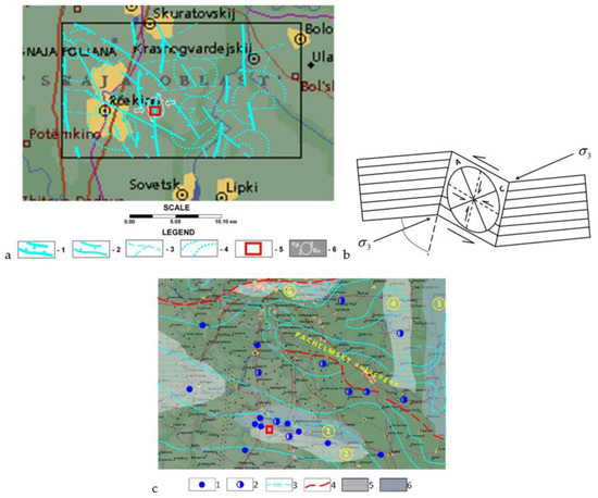
Figure 3.
The elements of regional geostructural reconstruction: (a) tracing the planetary fractures within the central part of the Tula region (1–4—different ranked elements of fault tectonics with ranking according to the degree of particular fracture fragmentation; 5—arch elements organized into ring structures; 6—position of investigated area; white lines reflect the reconstruction of normal stresses according to the model of deformation ellipsoid in the vicinity of investigated area marked by blue contour); (b) the model of deformation ellipsoid [39] with orientation of long axis of ellipsoid along bisector of acute angle between conjugated cracks (approximately under 60 degrees to each other) with shear kinematics; 3 s is the normal stresses; (c) fragment of tectonic map of the Russian Platform (according to K.Yu. Volkov [40]) (1—the wells uncovering the crystalline basement (numerator is the marker of depth of the roof, denominator includes total depth of drilling; 2—the wells where total depth of drilling is smaller than depth of crystalline basement roof; 3—isohypse of roof of crystalline basement according to combination of drilling data and seismic prospecting; 4—the same as “3” but according to the data of gravity survey; 5—deep fault; 6—local synforms; 7—local antiforms. Numbers in circles: 4—Trufano-Paveletskaya uplift zone; 5—Shchekino-Gorlovskaya zone of troughs; 6—Oksko-Tsinisky swell; 7—Vladimir-Shilovsky trough; 8—Moscow graben).
With regard to the submeridional geodynamic zone, there is the effect of shear displacement of elements of the geodynamic zone of the northwestern strike within the investigated area. Taking this into account, one can identify the northeastern strike of the axis along which the normal stresses are applied to the mining massif within the investigated area (Figure 3b). Then, applying the concept of conjugate fractures and the associated model of ellipsoid of deformations (Figure 3a), the generalized field of normal and shear stresses in projection onto the cartographical plane of the investigated territory is derived.
In mid-scale detailing of the geostructural image, trying to identify the generalized contour of the stressed rock massif, gradient operators and the generalization procedure discussed above were used. As a result, the image of the elliptical structure was mapped, fragmented along the set of sublatitudinal geodynamic zones, and along the zones of the northeastern strike and, to a lesser extent, the northwestern strike (Figure 4a). One can note the elliptical structure in Figure 4a surprisingly inherits the deformation ellipsoid shown in Figure 3a: there are coincidences both in the strike of the axes of the ellipses and in the distribution of the reconstructed normal and shear displacements which verify the mapped structural elements.
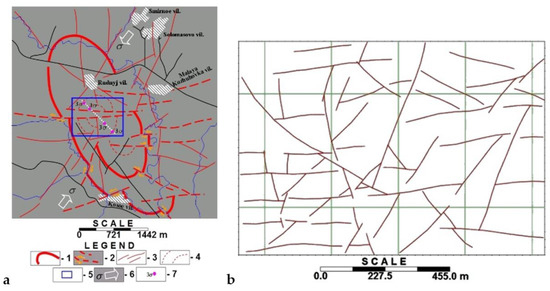
Figure 4.
Mid-scale and detailed geostructural reconstructions in the vicinity of the construction area: (a) detailing the image of ellipsoid of deformations (1—elliptical contour of stressed rock massif; 2—geodynamic zones with shear kinematics; 3—elements of fracture tectonics of unknown kinematics (low-contrast); 4—arch regional lineaments; 5—contour of investigated area; 6—normal stress; 7—generalized position of stress concentrators within investigated area); (b) large-scale geodynamic zones detailing based on combined decoding of remote sensing data (IR-band) and digital elevation model.
The contour of the elliptical structure is supposed to be the boundary of a certain weakened zone [41], which allows applying the analogy with the model of development of stress concentrators for localization of areas with an increased seismic hazard of the mining massif destruction. The mentioned model is related to the simplest mechanical formation, on the surface of which normal stresses σ are applied. It causes stress concentrators appearing in the bulk of the formation and in the small vicinity of the cavity (weakened zone), and the propagation of the zone of material plastic flow, developing into a crack. At the final stage of geostructural estimations in the cartographic plane, the large-scale data (approximately 1:14,000) were considered, reflected in Figure 4b. The smoothed morphology of the Earth’s relief implies the use of multiseason remote sensing images and digital elevation models in order to contrast the latest vertical subsidences within the investigated area.
The schematic map of geodynamic zones in Figure 5b is generalized up to the level of a lineament density map (Figure 3c) and verified at the stage of morphotectonic analysis (Figure 5a).
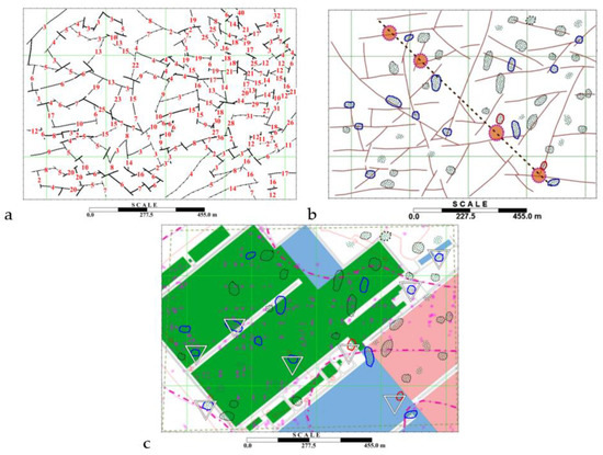
Figure 5.
Detailed morphostructural forecast: (a) geoblock fragmentation of the investigated area, reconstructed at the stage of morphotectonic analysis, combined with ranking elements (the boundaries are marked by the value of difference of average entropy value when moving from one geoblock to another); (b) forecast of zones of possible PES against the background of large-scale geostructural reconstruction (the most significant hazard areas: blue contours are the 3rd rank, marking the attraction to the nodes of intersection of geodynamic zones; red contours are the 4th rank of maximum significance, marking the attraction to mentioned detections as well as to the stress concentrators (orange circles)); (c) predictive map of positions of PES areas. The background of map reflects the principal position of boundaries of mine working; the pink dash-dotted line marks the zone of subsidence of rocks. The classification of PES areas of the 3rd and 4th rank (marked with triangles) is based on criterion of coincidence of the largest number of indicative detections.
First of all, one can see the manifestation of a ring structure in the map of geoblock structuring (Figure 5a), which verifies the middle-scale reconstructions (Figure 4a). The area of contact of more than two geoblocks is considered as a forecast marker with regard to the localization of areas of “Possible Earthquake Sources” (PES), where there is significant variation in theof entropy parameter (parameter of spatial stationarity of the Earth’s relief) (Figure 5b). At final stage of analysis, the ranked PES areas were compared with the lineament density map, where the maxima detected the areas of increased fragmentation of the geological environment. The coincidences of PES areas of the third and the fourth rank with the located maxima of the lineament density field were indicated by triangular markers and drawn in the final map of prognostic areas of the seismogenic hazard (Figure 5c). It is particularly remarkable that most of the selected PES areas were attracted to a priori specified zones of subsidence.
Considering the independence of decoding criteria, the combination of heterogeneous data (remote sensing images and digital elevation model) at different scale levels and the application of mutually verifying interpretation methods, the forecasting map in Figure 6c can be considered as the completed result requiring confirmation by geophysical estimations. Strictly speaking, this result is not the standard indicator adopted in the technology of seismic microzonation: using a combination of several parameters and recalculation methods, we just localize the region of reduced stability of the rock massif with no quantitative assessment of its stresses, displacements and increment in seismic intensity. Nevertheless, as we noted above, the problem is precisely in the localization of areas of a high seismic hazard for their subsequent quantitative description by more expensive methods of seismic microzonation.
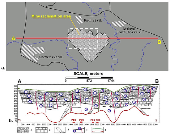
Figure 6.
The example of leading deep geostructural reconstruction along AB profile: (a) geographical reference of AB profile with regard to the boundaries of the area of interest; (b) image of geostructural reconstruction in vertical cross-section plane. The legend: 1,2—stratification elements; 3—through zones of increased permeability of geological environment; 4—interfaces (black—bedding, pink—fracture) and layer numbering; 5—roof and subface of reconstruction (green—the Earth’s relief, red—deep level of hydrostatic compensation of the Earth’s relief). The vertical green dotted line marks the boundaries of the area of interest. In the lower part of the section, the positions of PES zones are marked according to Figure 5c in projection on the AB profile. The scale of vertical and horizontal axes is defined in meters.
4. Discussion
Taking into account the last thesis about geophysical detailing, the interpretation procedure was extended by the solution to an inverse problem based on the recalculation of digital elevation models of the Earth’s relief in the volume of the geological environment. The final aim of this procedure was geostructural reconstruction in the plane of the vertical cross-section (Figure 6). The algorithm of recalculation used the wave analogies described above.
The profile line is drawn across the dominant strikes, reconstructed in Figure 5a,b. The area of interest is located in the center of this profile and occupies its fifth part: seeing a small step of discretization in the digital elevation model (it is about 0.5 m), this should allow both reconstruction of geostructural features in the investigated area and determining the presence of geostructural features of different ranks in the vicinity of this area.
In contrast to the reconstructions based on geophysical (seismic and electrical) data, in the considered case, the inverse problem is solved by the less rigorous model, in which the depth is computed as the relative parameter with application of empirical proportion between the linear size of landscape anomalies and the depth of their endogenous roots. The effect of multilevel isostatic compensation widely known in gravity prospecting is supposed to be the physical model: the larger the size of the positive or negative form of the Earth’s relief, the deeper the form hydrostatically compensated (see the Pratt and Airy model). The profile for deep reconstruction and, accordingly, for the selection of absolute heights of the Earth’s surface relief is chosen in the sublatitudinal direction, crossing the investigated area in its middle part (Figure 6a). The signal detail is the first meters, which allows speaking about the representativeness of the geostructural image in small parts of the cross-section. The selected PES areas are attracted to the zones of regional fault manifestation, to structural–constitutional complex thinning (sharp lateral variability of their composition) and to the elements of increased permeability zones. The deep reconstruction of the cross-section in Figure 6b is considered to be an independent way of presorting PES areas localized at the stage of reconstruction in the cartographic plane (Figure 5b). According to industrial experience, this approach is popular for estimation of objects for which there are no engineering and geophysical data due to limited access and a complicated landscape.
Upon achieving the leading forecast, the authors implemented seismic measurements within the industrial order (Figure 7), organized according to the “common depth point” (CDP) technique [42,43].
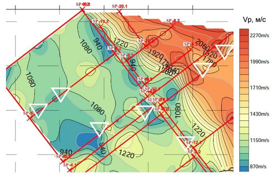
The measurement system was central, with no offset. The spacing between geophones was equal to 2.5 m, and the step of “VibroPoints” (VP) was equal to 5 m. A 48-channel array composed by SGD-AD ground geophones with an eigen frequency of 10 Hz was used. The increase in the CDP order at the junction of geophone arrays led to the application of an additional 12 VP along the flank observation system with variable offset from 2.5 to 57.5 m. Thus, the CDP order changed from 12 to 24 because of the low relative intensity of the target wave in the fractured rocks. Office processing of field data was carried out by RadExPro software, designed for integrated processing of data of surface engineering seismics as well as for quality control of field seismic data [44]. In total, during the processing, 21 sets of seismic determinations were identified, which fitted into three types of structuring of the velocity and depth propagation of the wave extremum: one—according to CDP, and two—according to the “refraction correlation method” (RCM). Following RCM interpretation, the layer which had the roof at the depth of 20 m and an increased velocity distribution within the range of 789–1317 m/s was selected. This layer had a widespread occurrence within the area of interest. The comparison of locations of the different ranked PES areas (see Figure 5c) and the negative anomalies of the P-wave velocity (zones of increased watering and deconsolidation, see Figure 7) demonstrates a significant spatial correlation. This correlation especially concerns PES zones of the third and the fourth rank as well as the result of their presorting according to the lineament density map. Thus, the objectivity of the result of the method of PES areas’ leading forecast based on qualitative and quantitative analysis of remote sensing data and digital elevation models of the Earth’s relief can be noted.
5. Conclusions
Investigations are completed based on a transition from small to large scales: from the location of the polygon position at the contact of Precambrian structures up to deriving the particular detections of regional faults in the vicinity of the area of interest. Despite the seismologically stable structural-tectonic position, this area is placed in the zone of widespread limestones, which causes karst development and a final reduction in the stability of the upper part of the geological cross-section. The karst development intensity and final high-amplitude subsidence of the Earth’s surface are associated with both the activation of tectonic faults and exogenous processes: against the background of fast-treated karstogenic formations, the appropriate erosion processes and watering initiate continuous dynamics of karst. These processes reflect the importance of the morphostructural and geodynamic analysis of remote sensing data and digital elevation models of the Earth’s surface, focused on mapping the inherited manifestation of elements of fracture tectonics and the geoblock structure. This analysis is especially effective under conditions of an initially smoothed relief and developed sea sediments widespread in the area of interest. The presented way of investigation includes qualitative and quantitative approaches to interpretation, where the first one is focused on lateral tracing of heterogeneities, whereas the second one is reduced to deep reconstruction. In the case of quantitative interpretation, a digital elevation model reflecting the functional dependence between the landscape and pre-Quaternary geology is considered within the concept of wave structuring of the Earth’s crust. The importance of the considered approach is explained by the data type—remote sensing data and digital elevation models are related to broad access materials for any continental part of the Earth’s crust. The mentioned lateral tracing is based on parametric decoding, solving the problem of tracing geodynamic zones and reconstruction of the geoblock structure as well as patterns in the stress field of the mining massif. The positions of possible focuses of secondary earthquakes are verified both by decoding at different scale levels and by applying functionally independent parametric estimations. Deep reconstructions are based on the wave model developed in publications by Petrov O.V. and Movchan I.B. [35], in which the jump-like changes in standing wavelengths are associated with the law of their dispersion and reflect the position of the interfaces in the stratified geological environment. The subvertical position of these interfaces is interpreted as the response of through zones of increased geological environment permeability. The correlation of possible sources of secondary earthquakes with the zones of increased permeability allows predicting areas of increased seismological magnitude with high reliability. Subsequent industrial activity by the shallow seismic technique confirms the reliability of PES areas localized at the stage of remote sensing data processing in combination with a digital elevation model.
Author Contributions
Contribution of authors to article preparation: I.B.M.: problem statement, field measurements, implementation of applied calculations, interpretation; A.B.M.: providing the project with remote sensing data, geological support of the project; A.A.Y.: applied programming, GIS design, geological and structural presentation of interpretation results. Z.I.S.: field measurements, development of maps. All authors have read and agreed to the published version of the manuscript.
Funding
This research is based on the grant of St. Petersburg Mining University KPD1-2020-165.
Institutional Review Board Statement
Not applicable.
Informed Consent Statement
Not applicable.
Data Availability Statement
The data are available on request from the corresponding author.
Conflicts of Interest
The authors declare the research was conducted in the absence of any commercial or financial relationships that could be construed as a potential conflict of interest.
References
- Rasulo, A.; Testa, K.; Borzi, B. Urban seismic risk analysis in Italy. In Computational Science and Its Applications—ICCSA 2015, Proceedings of the 15th International Conference, Banff, AB, Canada, 22–25 June 2015; Gervasi, O., Murgante, B., Misra, S., Gavrilova, M.L., Rocha, A.M.A.C., Torre, C., Taniar, D., Apduhan, B.O., Eds.; Springer: Cham, Switzerland, 2015; Volume 9157. [Google Scholar] [CrossRef]
- Ansal, A.; Kurtuluş, A.; Tönük, G. Seismic microzonation and earthquake damage scenarios for urban areas. Soil Dyn. Earthq. Eng. 2010, 30, 1319–1328. [Google Scholar] [CrossRef]
- Kurbatskiy, E.N.; Kosaurov, A.P. On the issue of recalculating seismic intensity points into ground-motion acceleration. J. Eng. Surv. 2016, 14, 50–60. [Google Scholar]
- Savitch, A.I.; Bugaevsky, A.G. Seismic microzoning for clarifying the parameters of seismic effects. J. Hydraul. Eng. 2015, 12, 53–58. Available online: http://www.gts.energy-journals.ru/index.php/GTS/article/view/326 (accessed on 1 May 2021).
- Cambazoglu, S.; Akgun, H.; Kockar, M.K. Preparation of a line source model for probabilistic seismic hazard analyses of Duzce Province, Turkey. In Proceedings of the 15th World Conference of Earthquake Engineering, Lisbon, Portugal, 24–28 September 2012. WCEE2012_3472. [Google Scholar]
- Harirchian, E.; Lahmer, T.; Rasulzade, S. Earthquake Hazard Safety Assessment of Existing Buildings Using Optimized Multi-Layer Perceptron Neural Network. Energies 2020, 13, 2060. [Google Scholar] [CrossRef]
- Soe, M.; Won-In, K.; Takashima, I.; Charusiri, P. Relationship between lineament density extraction from satellite image and earthquake distribution of Taungtonelone Area, Myanmar. In Proceedings of the 13rd CEReS International Symposium on Remote Sensing “Disaster Monitoring and Mitigation in Asia”, Chiba, Japan, 29–30 October 2007. [Google Scholar]
- Lister, G.; Tkalčić, H.; Hejrani, B.; Koulali, A.; Rohling, E.; Forster, M.; McClusky, S. Lineaments and earthquake ruptures on the East Japan megathrust. Lithosphere 2018, 10, 512–522. [Google Scholar] [CrossRef]
- Bondur, V.; Kuznetsova, L. Satellite monitoring of seismic hazard area geodynamics using the method of lineament analysis. In Proceedings of the 31st International Symposium on Remote Sensing of Environment, St. Petersburg, Russia, 20–24 June 2005. [Google Scholar]
- Yakovleva, A.A.; Movchan, I.B.; Misseroni, D.; Pugno, N.M. Multi-Physics of Dynamic Elastic Metamaterials and Earthquake Systems. J. Front. Mater. 2021, 7, 489. [Google Scholar] [CrossRef]
- Eppelbaum, L.V. Localization of ring structures in Earth’s environment. J. Archaeol. Soc. Slovak. Acad. Sci. 2007, 41, 145–148. Available online: https://www.researchgate.net/publication/231817311 (accessed on 1 May 2021).
- Koronovsky, N.V.; Bryantseva, G.V.; Goncharov, M.A.; Naimark, A.A.; Kopaev, A.V. Lineaments, planetary jointing, and the regmatic system: Main points of the phenomena and terminology. Geotectonics 2014, 48, 151–162. [Google Scholar] [CrossRef]
- Ford, D.C.; Williams, P.W. Karst Hydrogeology and Geomorphology; Revised Edition; Wiley: New York, NY, USA, 2007. [Google Scholar]
- Ulomov, V.I.; Bogdanov, M.I. On the software and mathematical support for development of the maps of probabilistic seismic zoning according to OSR-97 technique. Geophysical research: Collection of scientific papers of the Institute of Physics of the Earth. RAS 2007, 7, 29–52. [Google Scholar]
- Giardini, D.; Gruenthal, G.; Shedlock, K.; Zhang, P. The GSHAP global seismic hazard map. J. Int. Geophys. 2003, 81, 1239–1244. [Google Scholar] [CrossRef]
- Gospodarikov, A.P.; Chi, T.N. The impact of earthquakes on the tunnel from Hanoi metro system when the tunnel has a horseshoe shape cross-section. Int. J. Civ. Eng. Technol. 2019, 10, 79–86. Available online: http://www.iaeme.com/IJCIET/issues.asp?JType=IJCIET&VType=10&IType=2 (accessed on 1 May 2021).
- Kheraskova, T.N.; Andreeva, N.K.; Vorontsov, A.K.; Kagramanyan, A. Evolution of the Moscow sedimentary basin in the early Paleozoic. J. Lithol. Miner. Resour. 2005, 40, 150–166. [Google Scholar] [CrossRef]
- Sokolov, E.M.; Dmitrakov, A.V.; Simakin, A.F.; Reshetov, V.V. Geoecology of the Economic Complex of Tula and Its Region; Tula State University: Tula, Russia, 2000; 110p. [Google Scholar]
- Danilev, S.M.; Danileva, N.A. Characteristics electromagnetic waves of GPR data for study of hidden cavities in the engineering objects. In Engineering and Mining Geophysics 2018, Proceedings of the 14th Conference and Exhibition on Engineering and Mining Geophysics 2018, Almaty, Kazakhstan, 23–27 April 2018; European Association of Geoscientists & Engineers: Houten, The Netherlands, 2018; Volume 2018, pp. 1–4. [Google Scholar] [CrossRef]
- Danilev, S.M.; Danileva, N.A. Perspective electrical exploration the dams of gypsum accumulator in the framework for geotechnical monitoring. In Engineering and Mining Geophysics 2019, Proceedings of the 15th Conference and Exhibition on Engineering and Mining Geophysics 2019, Gelendzhik, Russia, 16 April 2019; European Association of Geoscientists & Engineers: Houten, The Netherlands, 2019; Volume 2019, pp. 1–7. [Google Scholar] [CrossRef]
- Ostrovskaya, E.V. Some problems of ecology of natural waters of Novomoskovsk district of Tula region. J. Min. Inst. 2002, 152, 39–41. Available online: http://pmi.spmi.ru/index.php/pmi/article/view/9324?setLocale=en_US (accessed on 1 May 2021).
- Afanasiadi, E.I.; Gryaznov, O.N.; Dubeykovsky, S.G.; Neshetkin, O.B. Limestone Karst of the East Ural Region. J. Min. Inst. 2003, 153, 46–50. Available online: http://pmi.spmi.ru/index.php/pmi/article/view/9243 (accessed on 1 May 2021).
- Pashkevich, M.; Petrova, T.A. Development of an operational environmental monitoring system for hazardous industrial facilities of Gazprom Dobycha Urengoy. J. Phys. Conf. Ser. 2019, 1384, 1–7. [Google Scholar] [CrossRef]
- Egorov, A.S.; Vinokurov, I.Y.; Belevskaya, E.S.; Kalenich, A.P. Deep structure of the Barents-Kara region according to geophysical investigations along 1-AR and 2-AR geotravers. In Understanding the Harmony of the Earth’s Resources through Integration of Geosciences, Proceedings of the 7th Eage Saint Petersburg International Conference and Exhibition, St. Petersburg, Russia, 11–14 April 2016; European Association of Geoscientists & Engineers: Houten, The Netherlands, 2016; pp. 728–732. [Google Scholar] [CrossRef]
- Rakhil, K.R.; Kishan, D.; Sarup, J. Lineament extraction and lineament density assessment of Omkareshwar, M P, India, using GIS Techniques. Int. J. Eng. Manag. Res. 2015, 5, 717–720. [Google Scholar] [CrossRef][Green Version]
- Gupta, R.P. Remote Sensing: Geology, 2nd ed.; Springer: Berlin/Heidelberg, Germany, 2003; 656p. [Google Scholar] [CrossRef]
- Nugroho, U.C.; Tjahjaningsih, A. Lineament density information extraction using dem srtm data to predict the mineral potential zones. Int. J. Remote Sens. Earth Sci. 2016, 13, 67–74. [Google Scholar] [CrossRef][Green Version]
- Kennelly, P.J. Terrain maps displaying hill-shading with curvature. J. Geomorphol. 2008, 102, 567–577. [Google Scholar] [CrossRef]
- Dahlhaus, R.; Kurths, J.; Maass, P.; Timmer, J. Mathematical Methods in Time Series Analysis and Digital Image Processing; Springer: Berlin/Heidelberg, Germany, 2021; 73p. [Google Scholar] [CrossRef]
- Núñez, I.; Ferrari, J.A. Differential operator approach for Fourier image processing. J. Opt. Soc. Am. 2007, 24, 2274–2279. [Google Scholar] [CrossRef]
- Singhroy, V.H.; Pilkington, M. Geological mapping using earth’s magnetic field. In Encyclopedia of Remote Sensing; Springer: New York, NY, USA, 2014; pp. 232–237. [Google Scholar]
- Grazzini, J.; Turiel, A.; Yahia, H. Entropy estimation and multiscale processing in meteorological satellite images. In Proceedings of the 16th International Conference on Pattern Recognition, Quebec City, QC, Canada, 11–15 August 2002; Volume 3. [Google Scholar]
- Muhammad, E.M.N.; Muhammad, S.S.; Arif, H.; Wildan, N.H.; Benyamin, S.; Mirzam, A.; Alfend, R. Automatic and manual fracture-lineament identification on digital surface models as methods for collecting fracture data on outcrops: Case study on fractured granite outcrops, Bangka. J. Front. Southeast Asian Geosci. 2020, 8, 560596. [Google Scholar] [CrossRef]
- Petrov, O.V. The Earth’s Dissipative Structures: Fundamental Wave Properties of Substance; Springer: Cham, Switzerland, 2019; pp. 23–57. [Google Scholar] [CrossRef]
- Petrov, O.V. The Earth’s Free Oscillations; Springer: Cham, Switzerland, 2021; 107p. [Google Scholar] [CrossRef]
- Petrakov, D.; Kupavykh, K.; Kupavykh, A. The effect of fluid saturation on the elastic-plastic properties of oil reservoir rocks. Curved Layer. Struct. 2020, 7, 29–34. [Google Scholar] [CrossRef]
- Ribe, N.M. Bending and stretching of thin viscous sheets. J. Fluid Mech. 2001, 433, 135–160. [Google Scholar] [CrossRef]
- Aleksanova, E.D.; Varentsov, I.M.; Vereshchagina, M.I.; Kulikov, V.A.; Pushkarev, P.Y.; Sokolova, E.Y.; Shustov, N.L.; Khmelevskoi, V.K.; Yakovlev, A.G. Electromagnetic soundings of the sedimentary cover and consolidated crust in the transition zone from the Moscow syneclise to the Voronezh anteclise: Problems and prospects. J. Izv. Phys. Solid Earth 2010, 46, 707–716. [Google Scholar] [CrossRef]
- Mulchrone, K.F.; Talbot, C.J. Constraining the strain ellipsoid and deformation parameters using deformed single layers: A computational approach assuming pure shear and isotropic volume change. J. Struct. Geol. 2014, 52, 194–206. [Google Scholar] [CrossRef]
- Volkov, K.Y. Schematic Map of Roof Relief of Crystalline Basement of Moscow Syneclise and Ryazan-Saratov Trough; GURTs: Moscow, Russia, 1965. [Google Scholar]
- Mazurov, B.T.; Mustafin, M.G.; Panzhin, A.A. Estimation method for vector field divergence of Earth crust deformations in the precess of Mineral deposits development. Zap. Gorn. Inst./J. Min. Inst. 2019, 238, 376–382. [Google Scholar] [CrossRef]
- Gorelik, G.D.; Budanov, L.M.; Ryabchuk, D.; Zhamoida, V.; Neevin, I. Application of CDP seismic reflection method in buried paleo-valley study. In Engineering and Mining Geophysics 2019, Proceedings of the 15th Conference and Exhibition on Engineering and Mining Geophysics 2019, Gelendzhik, Russia, 16 April 2019; European Association of Geoscientists & Engineers: Houten, The Netherlands, 2019; Volume 2019, pp. 1–7. [Google Scholar] [CrossRef]
- Sloan, S.D.; Tsoflias, G.P.; Steeples, D.W. Ultra-shallow seismic imaging of the top of the saturated zone. Geophys. Res. Lett. 2010, 37, 4453. [Google Scholar] [CrossRef]
- Lalomov, D.; Glazunov, V.; Tatarskiy, A.; Burlutsky, S.; Efimova, N. Methodical features of studying the geological structure of the coastal part of the sea of Okhotsk based on the integration of continuous aquatic electrical sounding and seismoacoustics data. In Proceedings of the 25th European Meeting of Environmental and Engineering Geophysics, Held at Near Surface Ge-oscience Conference and Exhibition 2019, NSG 2019, The Hague, The Netherlands, 8–12 September 2019; European Associa-tion of Geoscientists and Engineers: Houten, The Netherlands, 2019; Volume 2019, pp. 1–5. [Google Scholar]


Publisher’s Note: MDPI stays neutral with regard to jurisdictional claims in published maps and institutional affiliations. |
© 2021 by the authors. Licensee MDPI, Basel, Switzerland. This article is an open access article distributed under the terms and conditions of the Creative Commons Attribution (CC BY) license (https://creativecommons.org/licenses/by/4.0/).