Author Contributions
M.H.: methodology, software, investigation, data curation, writing – original draft preparation, visualization; D.V.: conceptualization, methodology, validation, investigation, writing – review and editing, supervision; R.M.: conceptualization, methodology, validation, investigation, data curation, writing – review and editing, supervision. All authors have read and agreed to the published version of the manuscript.
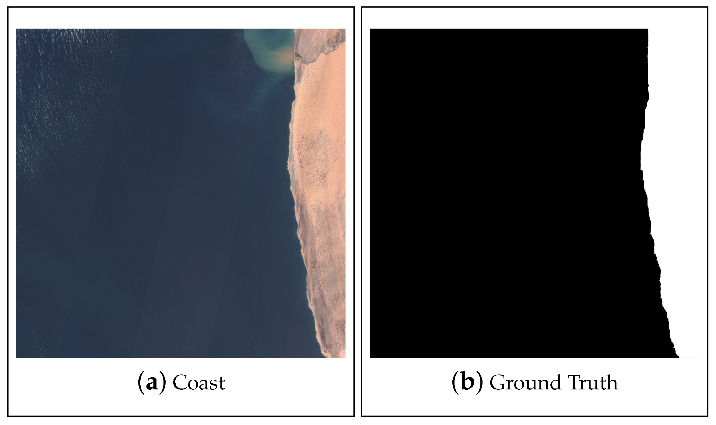
Figure 1.
Image number 12 to be evaluated with corresponding ground truth.
Figure 1.
Image number 12 to be evaluated with corresponding ground truth.
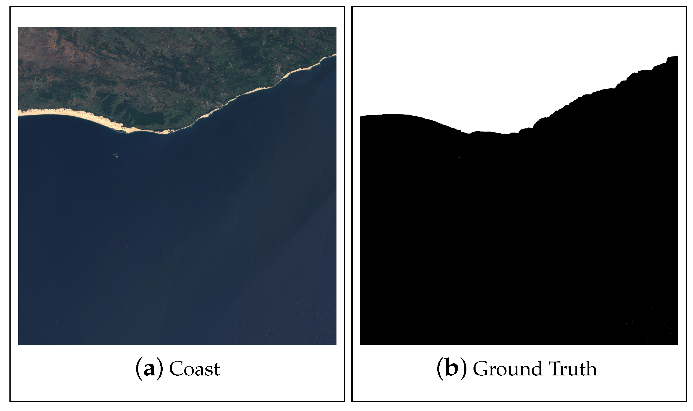
Figure 2.
Image number 18 to be evaluated with corresponding ground truth.
Figure 2.
Image number 18 to be evaluated with corresponding ground truth.
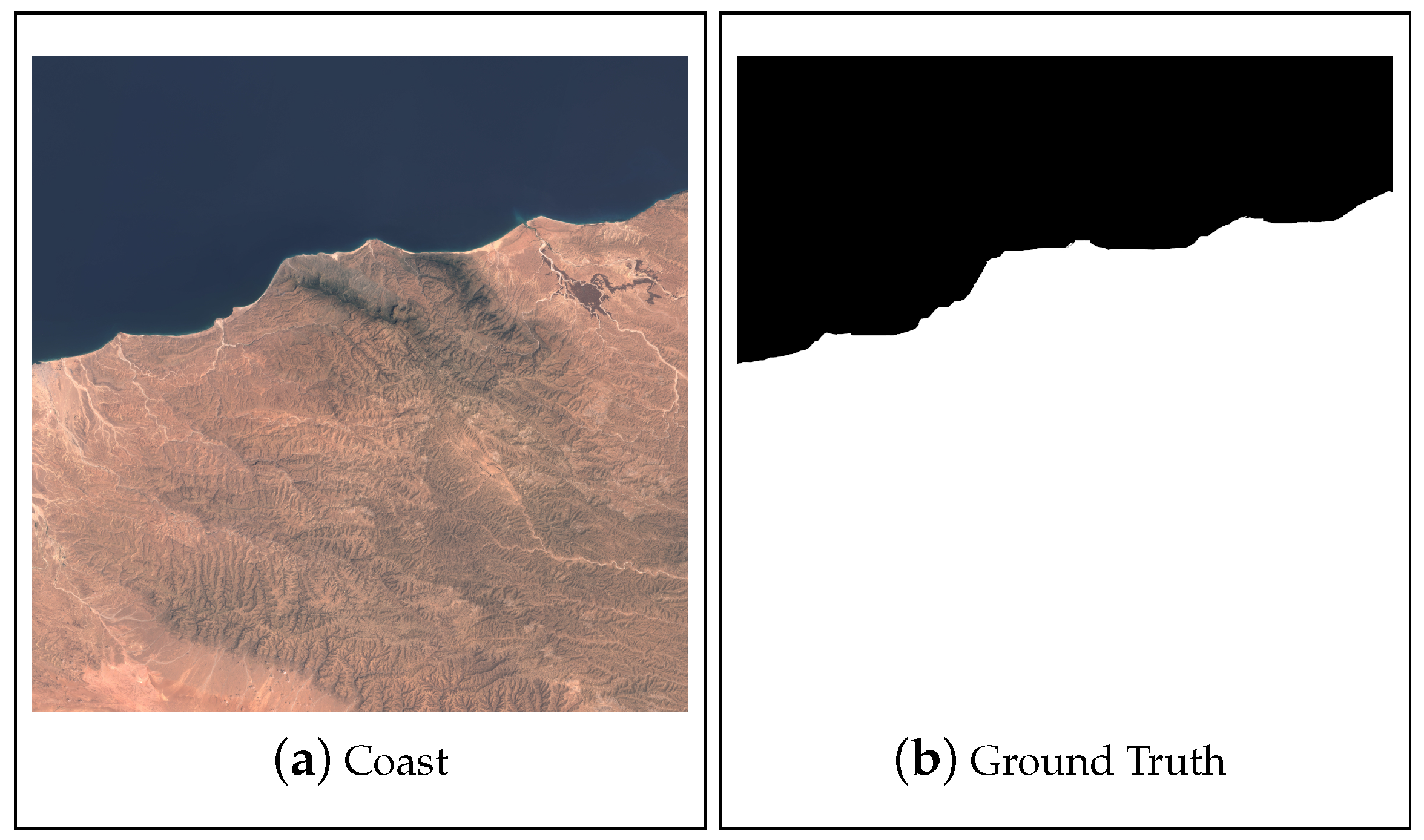
Figure 3.
Image number 27 to be evaluated with corresponding ground truth.
Figure 3.
Image number 27 to be evaluated with corresponding ground truth.
Figure 4.
Image number 38 to be evaluated with corresponding ground truth.
Figure 4.
Image number 38 to be evaluated with corresponding ground truth.
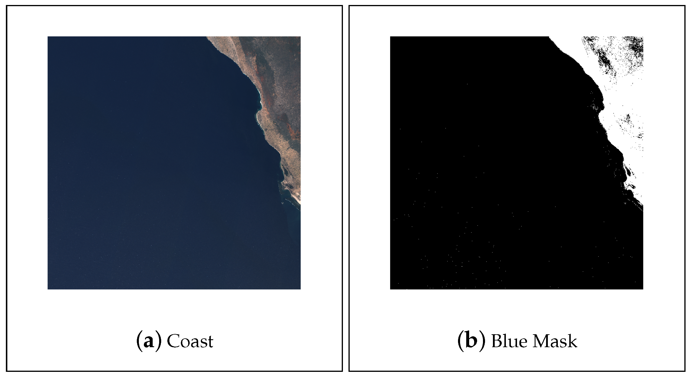
Figure 5.
Original image and Blue Mask of Coast_D(23).jpg.
Figure 5.
Original image and Blue Mask of Coast_D(23).jpg.
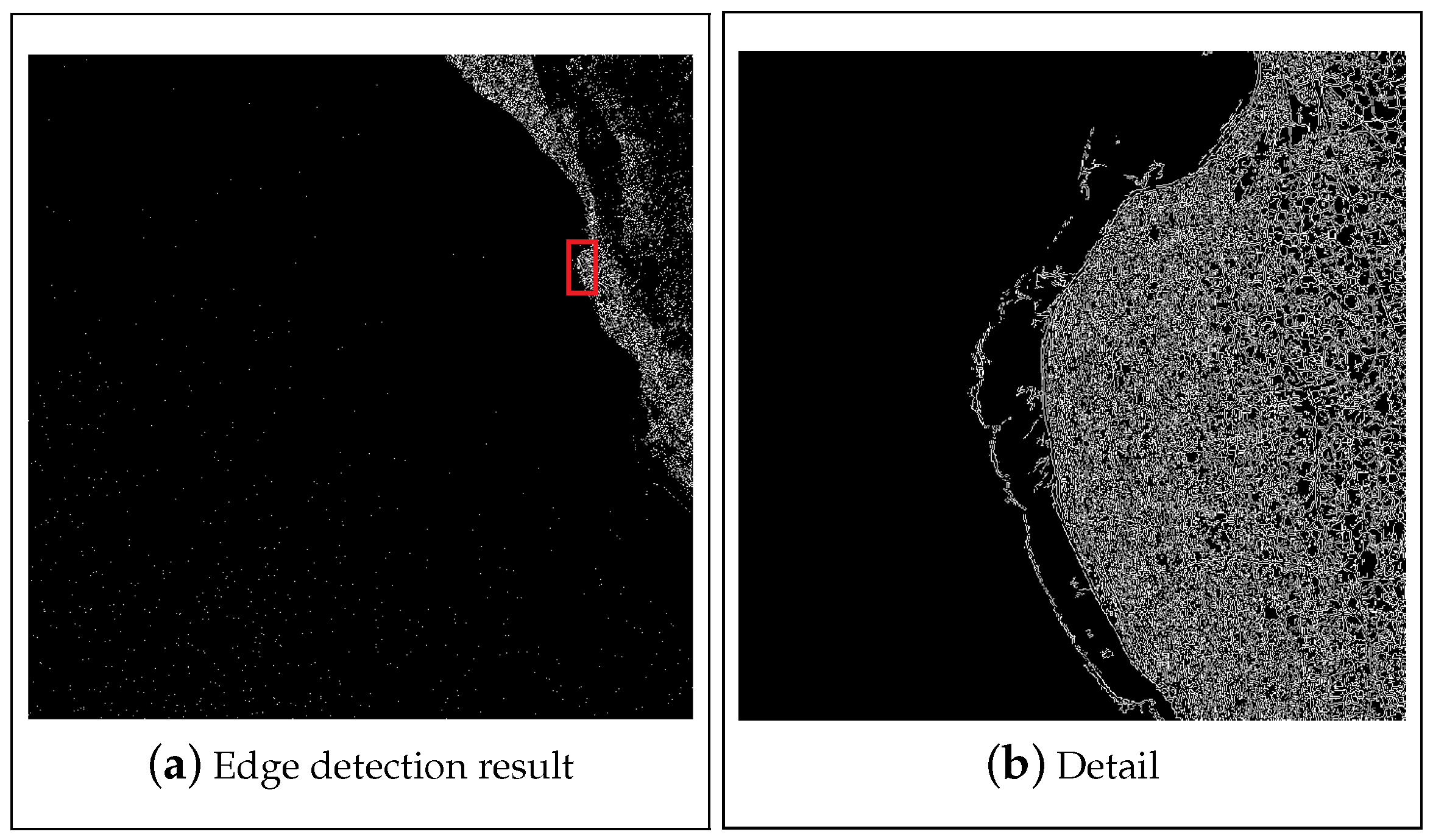
Figure 6.
Output of an edge detection operation.
Figure 6.
Output of an edge detection operation.
Figure 7.
Totally Processed Image.
Figure 7.
Totally Processed Image.
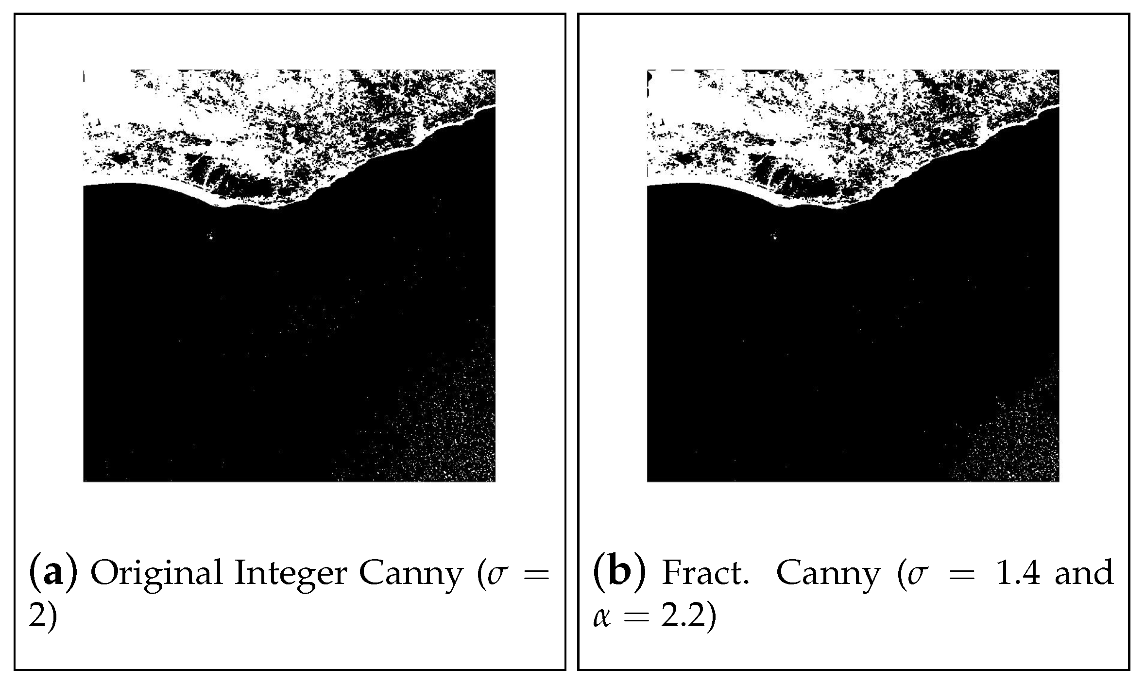
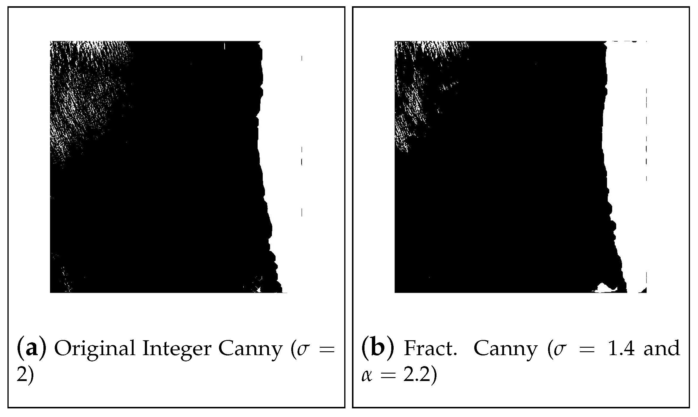
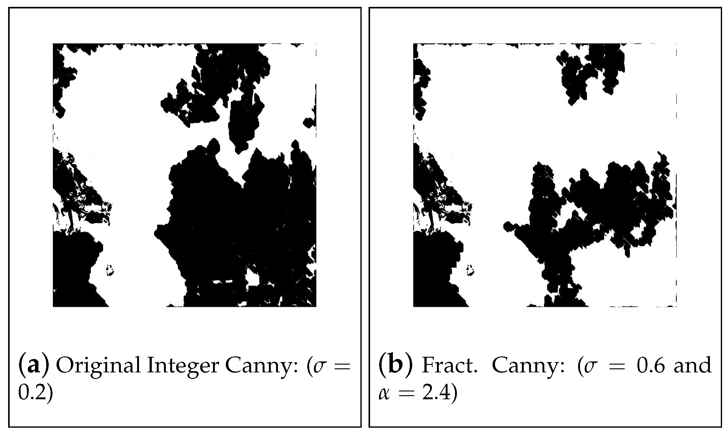
Figure 8.
Best results for image 12 processed using Canny algorithms.
Figure 8.
Best results for image 12 processed using Canny algorithms.
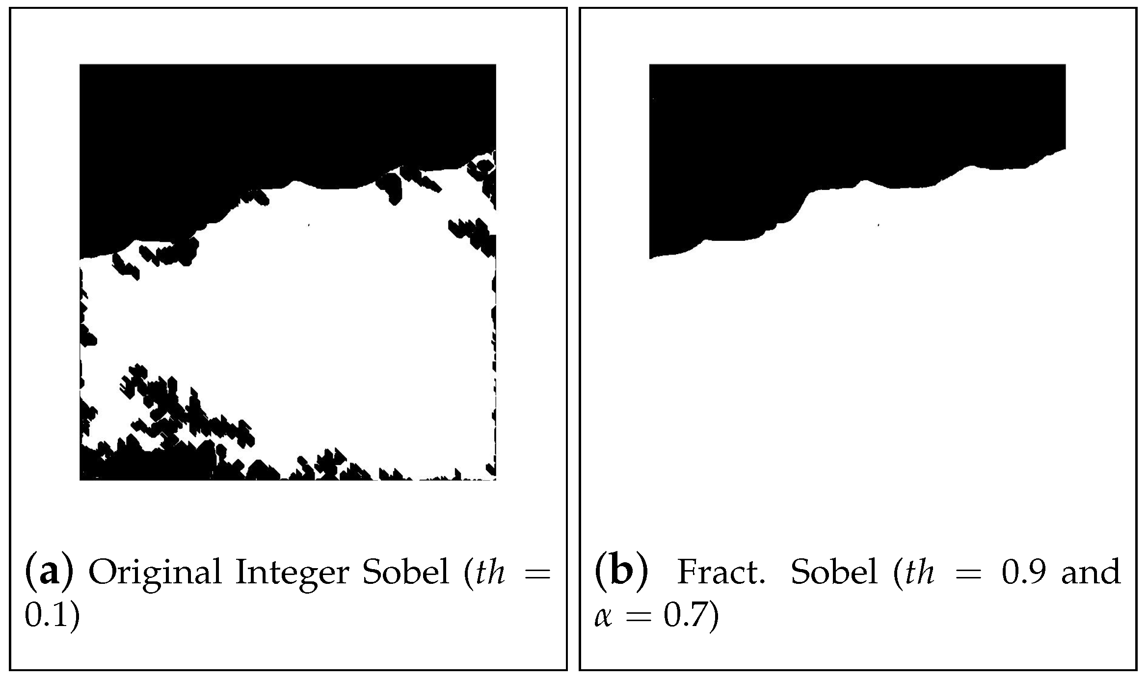
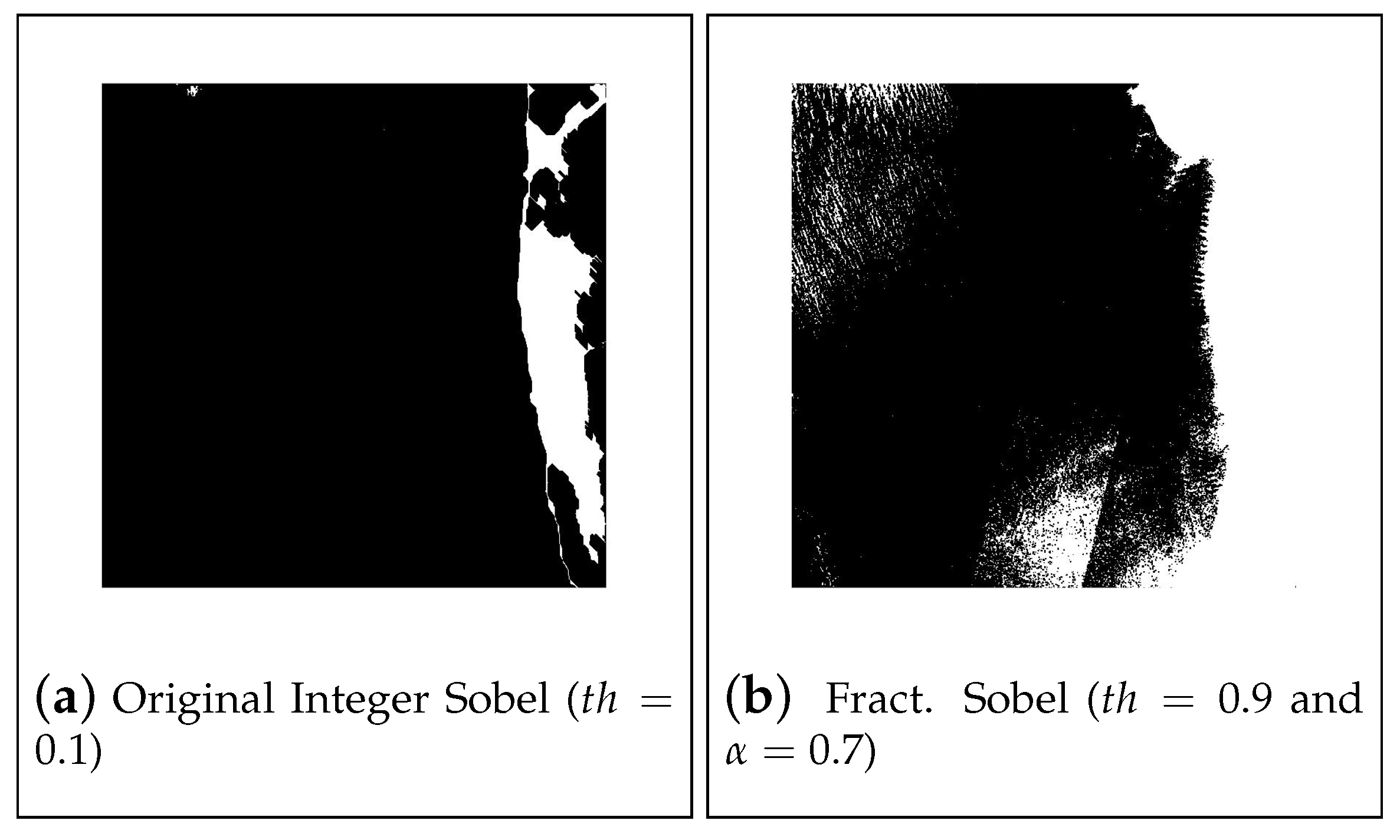
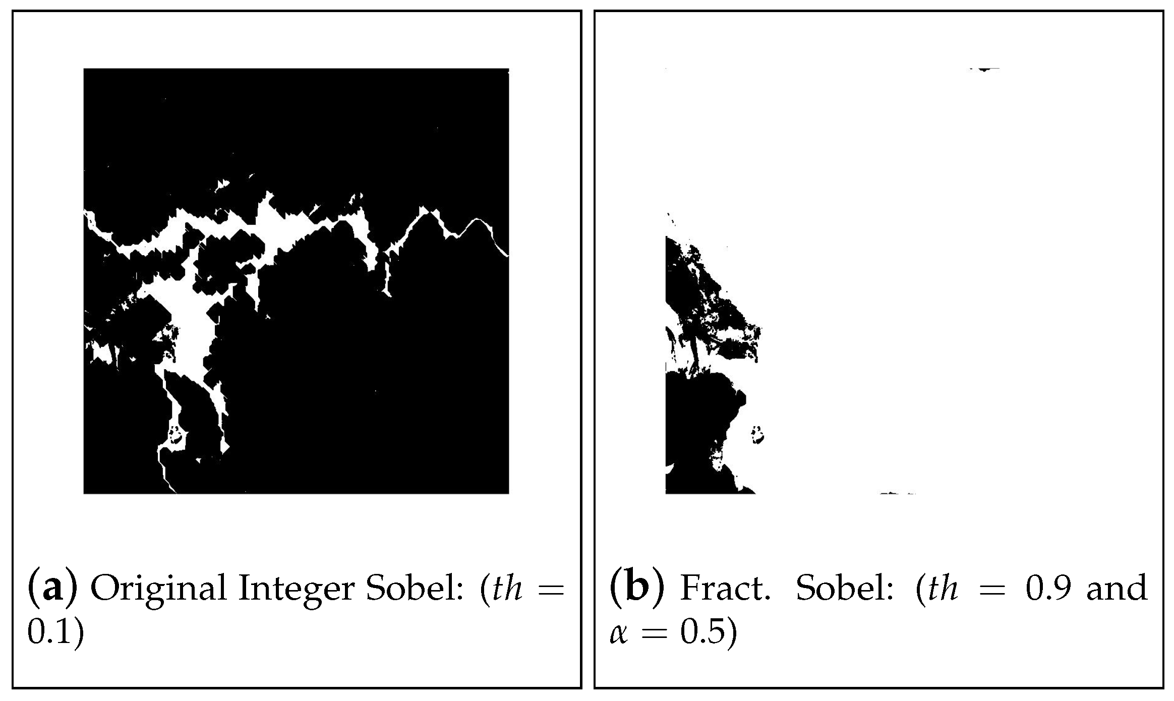
Figure 9.
Best results for image 12 processed using Sobel algorithms.
Figure 9.
Best results for image 12 processed using Sobel algorithms.
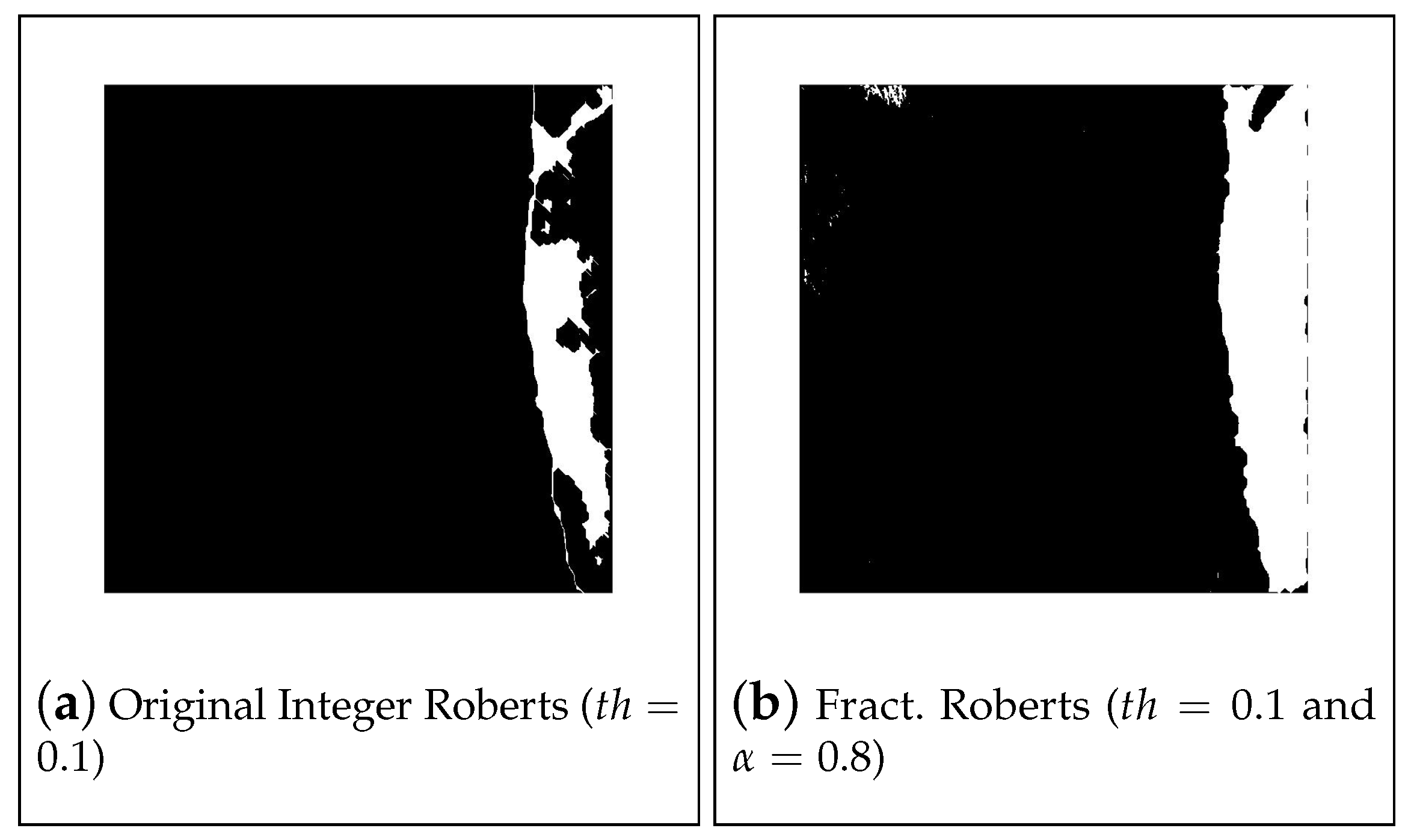
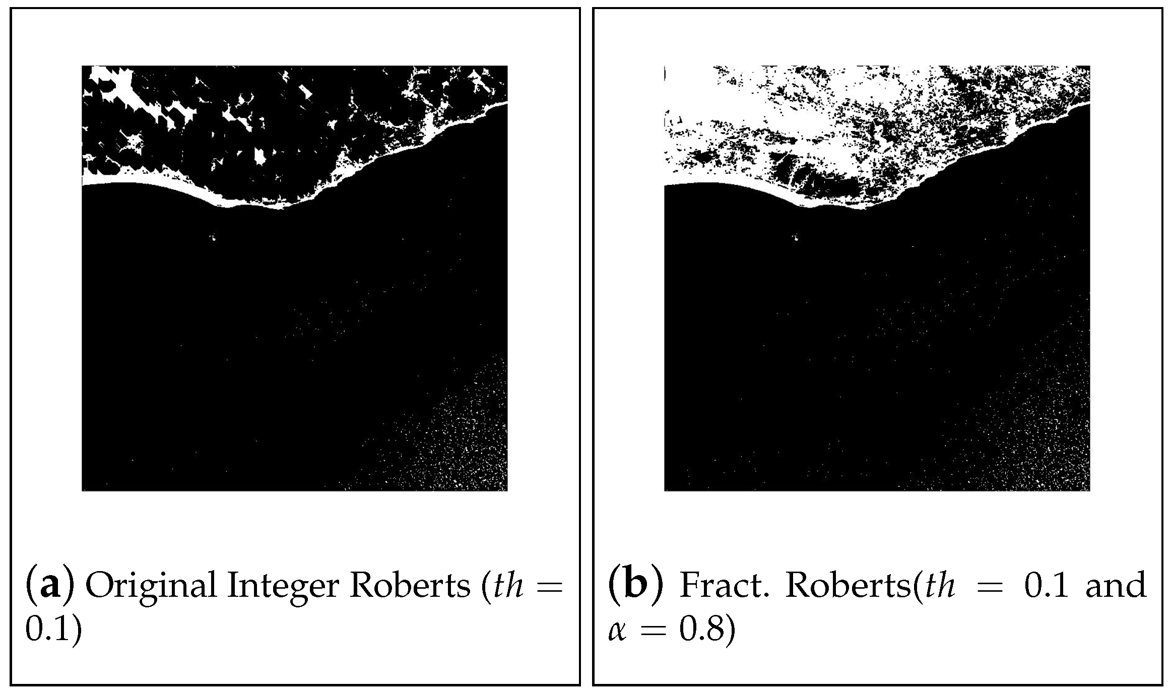
Figure 10.
Best results for image 12 processed using Roberts algorithms.
Figure 10.
Best results for image 12 processed using Roberts algorithms.
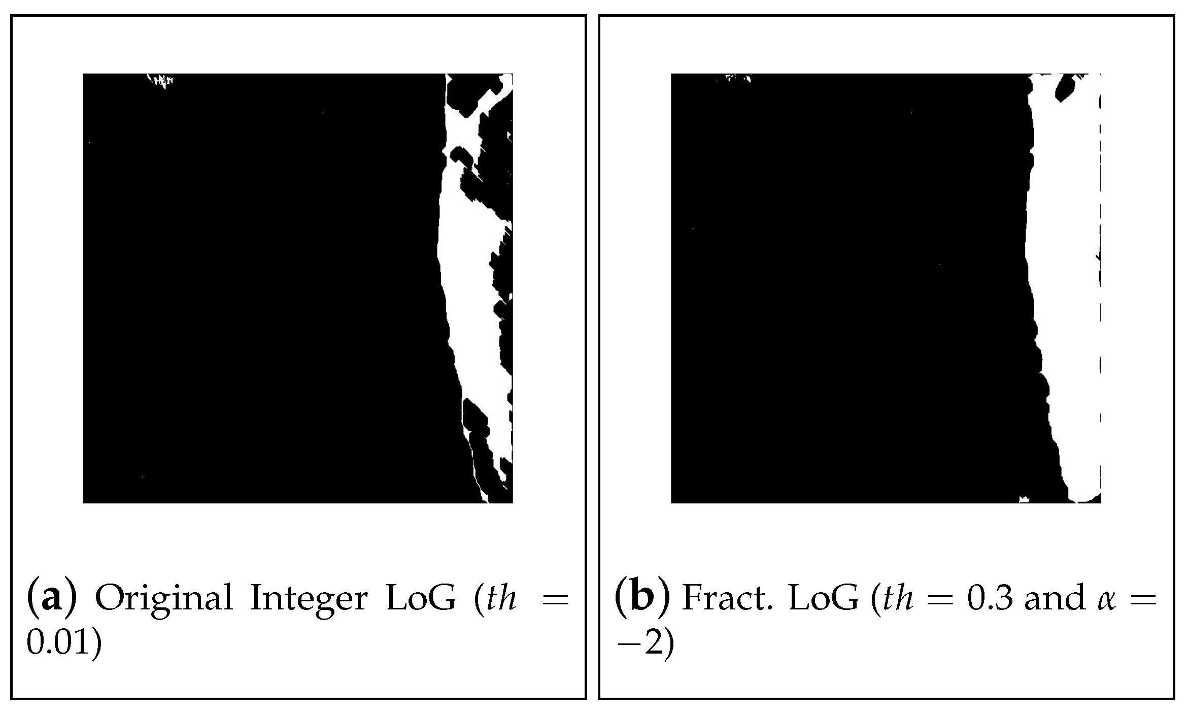
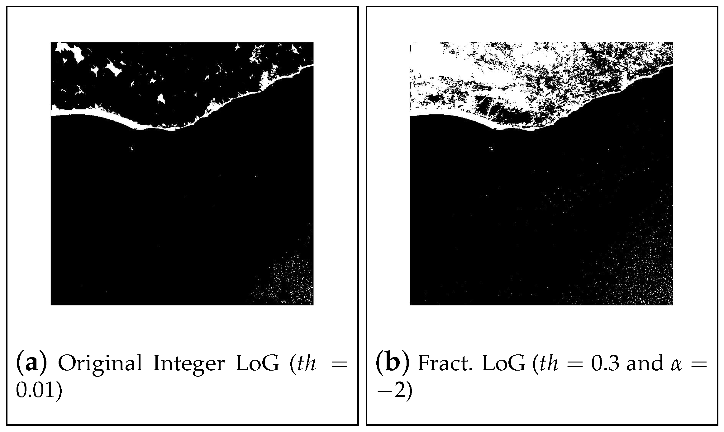
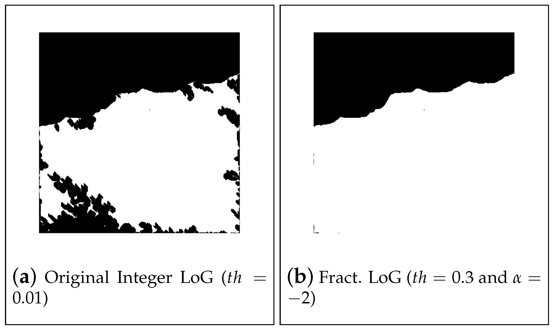
Figure 11.
Best results for image 12 processed using LoG algorithms.
Figure 11.
Best results for image 12 processed using LoG algorithms.
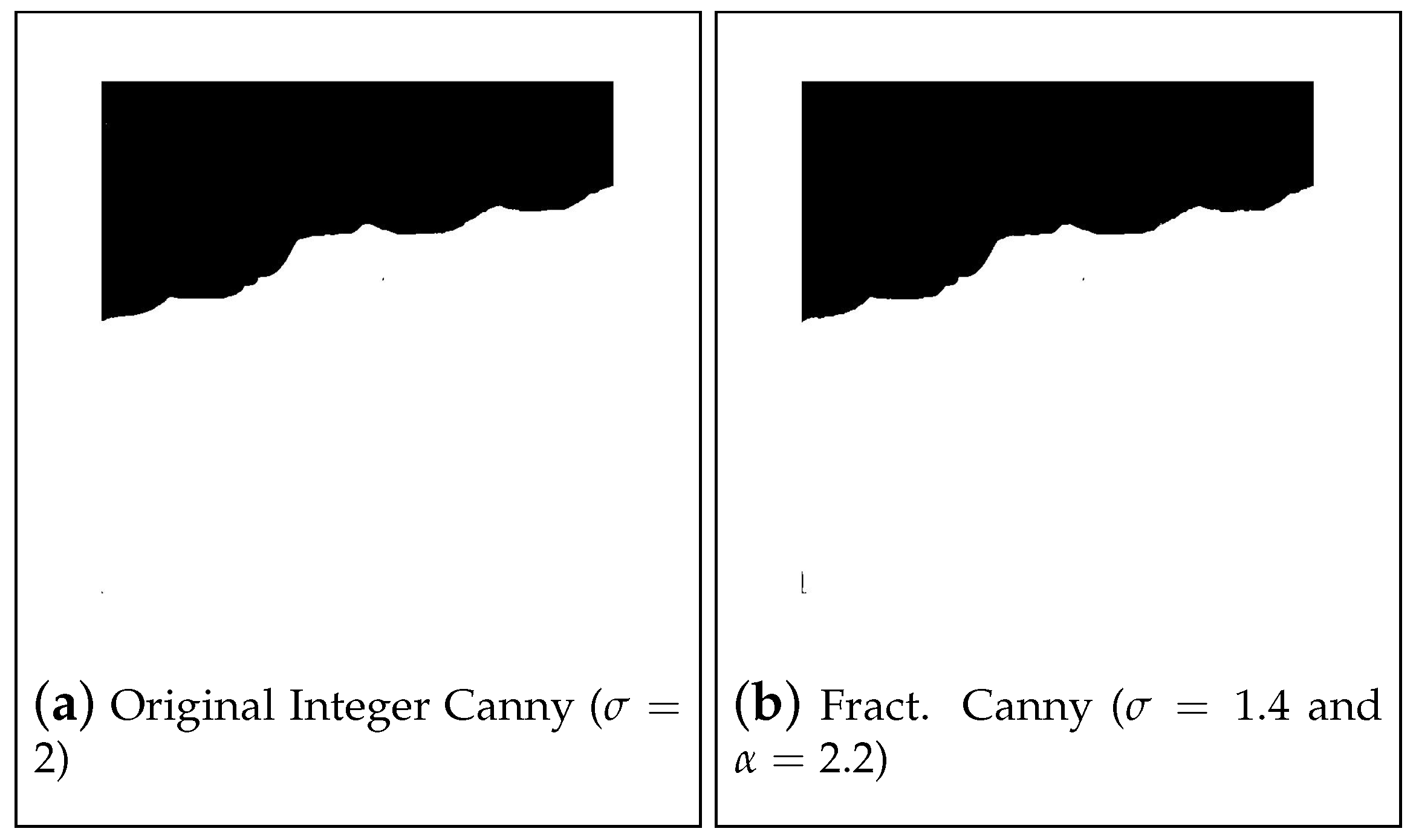
Figure 12.
Best results for image 18 processed using Canny algorithms.
Figure 12.
Best results for image 18 processed using Canny algorithms.
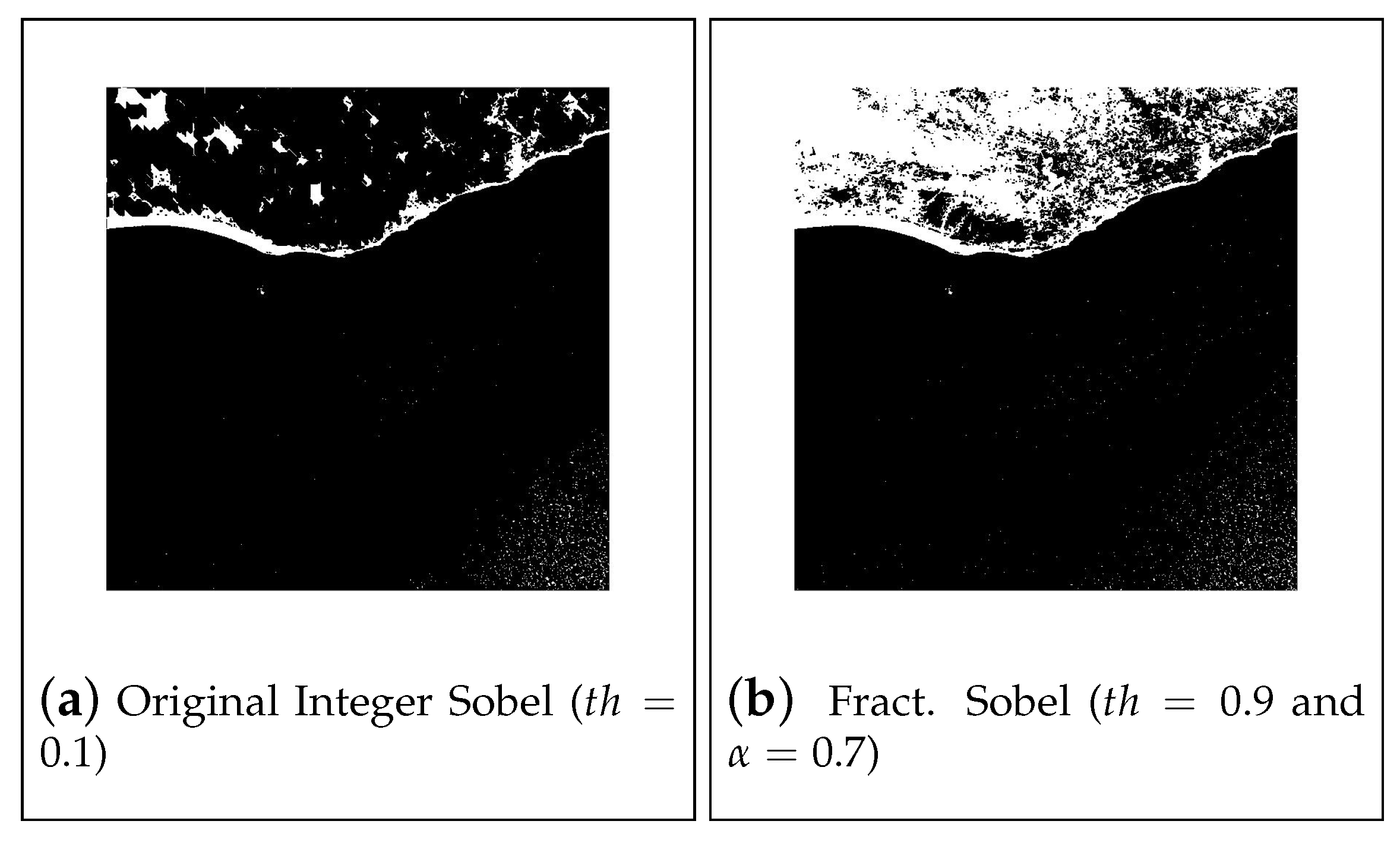
Figure 13.
Best results for image 18 processed using Sobel algorithms.
Figure 13.
Best results for image 18 processed using Sobel algorithms.
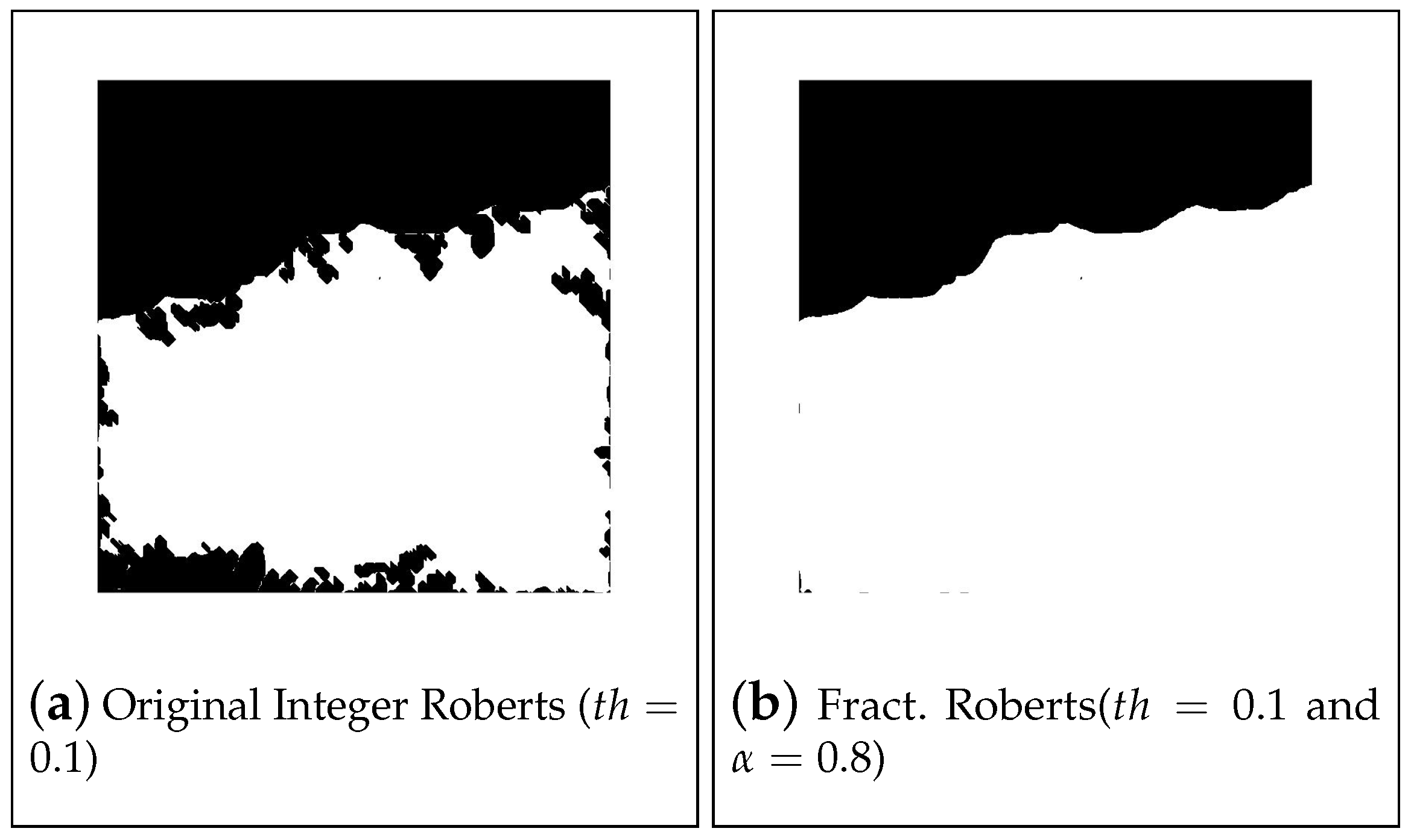
Figure 14.
Best results for image 18 processed using Roberts algorithms.
Figure 14.
Best results for image 18 processed using Roberts algorithms.
Figure 15.
Best results for image 18 processed using LoG algorithms.
Figure 15.
Best results for image 18 processed using LoG algorithms.
Figure 16.
Best results for image 27 processed using Canny algorithms.
Figure 16.
Best results for image 27 processed using Canny algorithms.
Figure 17.
Best results for image 27 processed using Sobel algorithms.
Figure 17.
Best results for image 27 processed using Sobel algorithms.
Figure 18.
Best results for image 27 processed using Roberts algorithms.
Figure 18.
Best results for image 27 processed using Roberts algorithms.
Figure 19.
Best results for image 27 processed using LoG algorithms.
Figure 19.
Best results for image 27 processed using LoG algorithms.
Figure 20.
Best results for image 38 processed using Canny algorithms.
Figure 20.
Best results for image 38 processed using Canny algorithms.
Figure 21.
Best results for image 38 processed using Sobel algorithms.
Figure 21.
Best results for image 38 processed using Sobel algorithms.
Figure 22.
Best results for image 38 processed using Roberts algorithms.
Figure 22.
Best results for image 38 processed using Roberts algorithms.
Figure 23.
Best results for image 38 processed using LoG algorithms.
Figure 23.
Best results for image 38 processed using LoG algorithms.
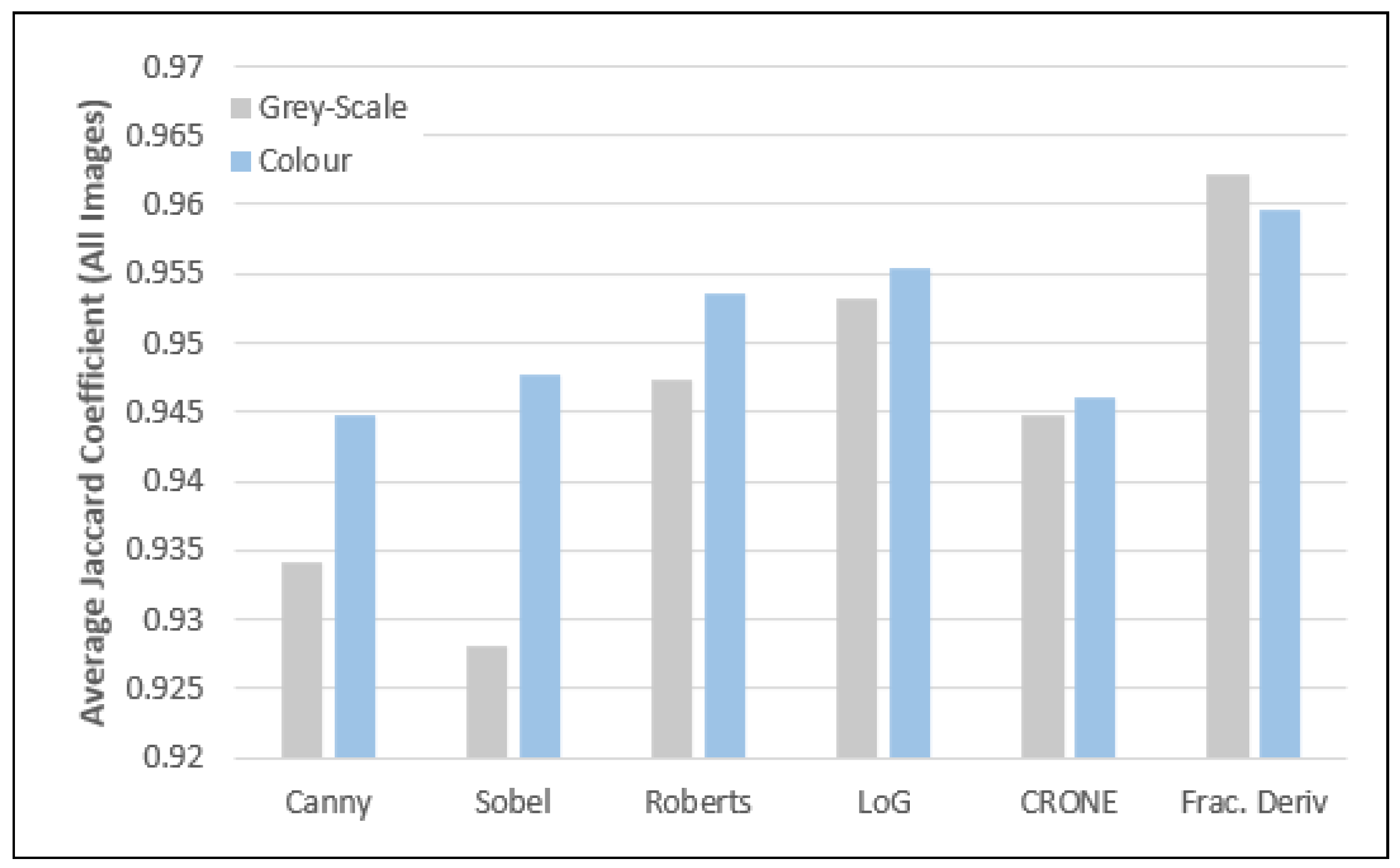
Figure 24.
Analysis of performance comparison between grey-scale and color based detectors.
Figure 24.
Analysis of performance comparison between grey-scale and color based detectors.
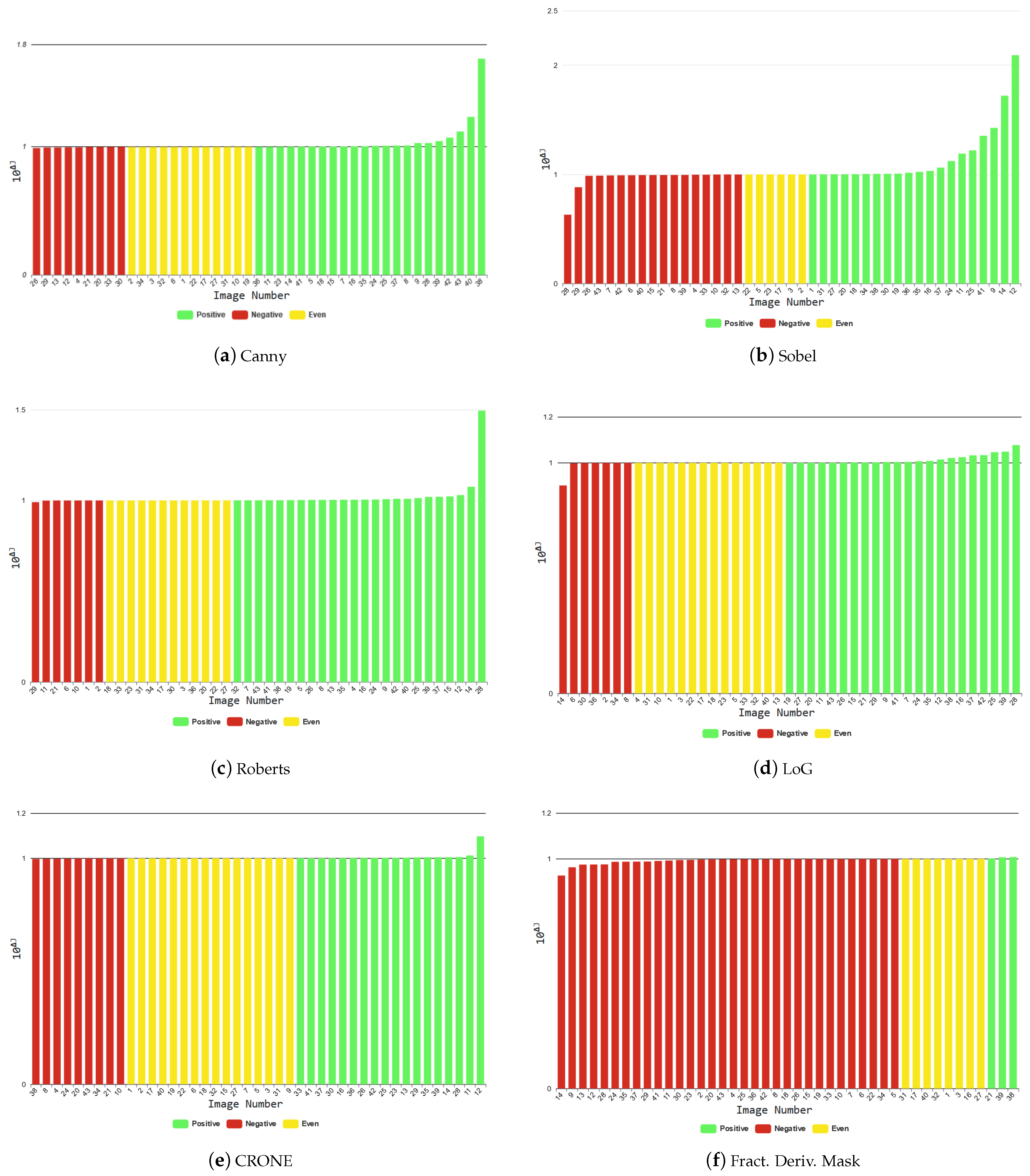
Figure 25.
Bar chart with best results average for all images (Varying parameters).
Figure 25.
Bar chart with best results average for all images (Varying parameters).
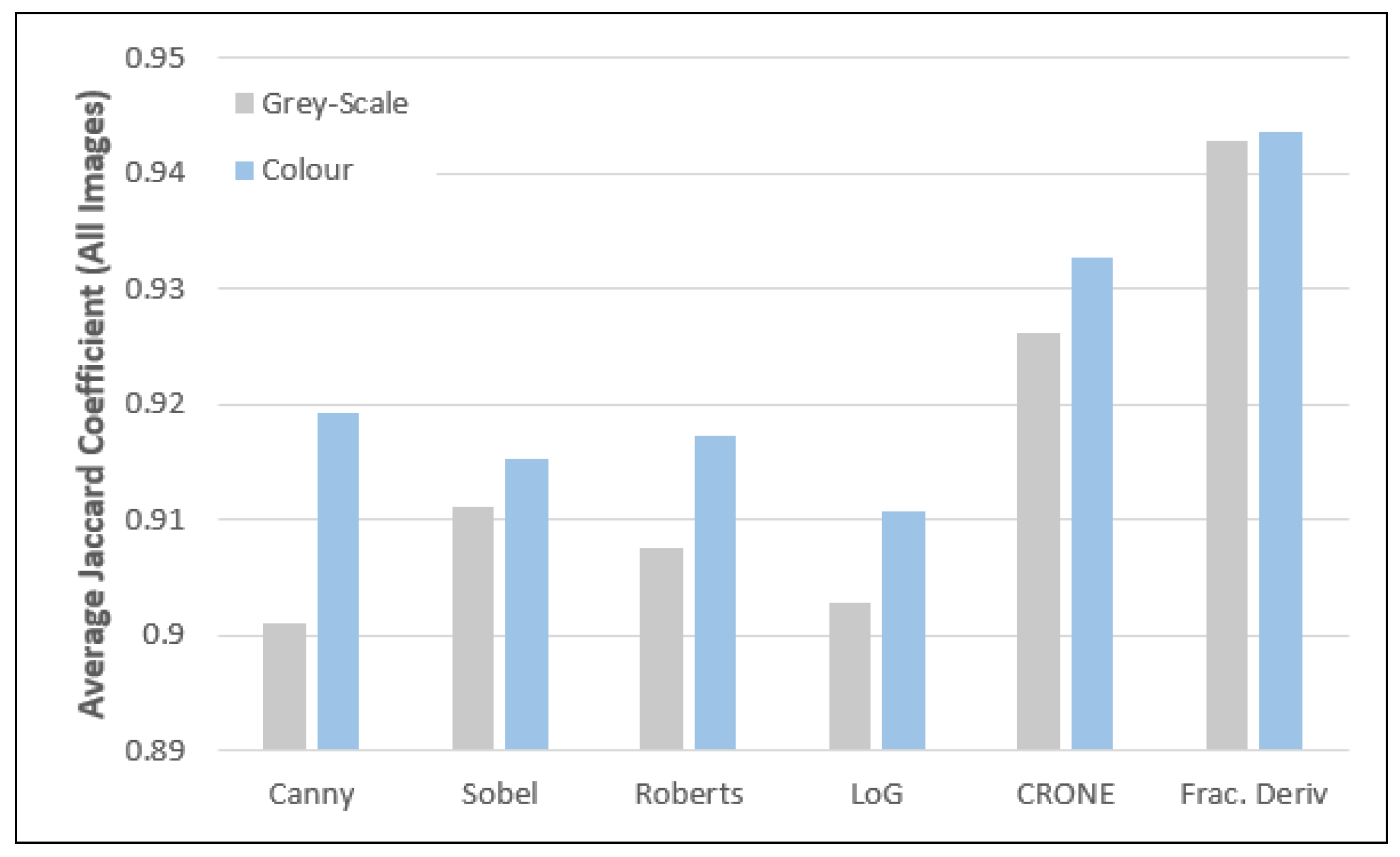
Figure 26.
Bar chart with best results average for all images (Fixed parameters).
Figure 26.
Bar chart with best results average for all images (Fixed parameters).
Table 1.
Performance Instances.
Table 1.
Performance Instances.
| | Processed Image |
|---|
| | | | 0 | 1 |
| Ground Truth | | 0 | TN | FP |
| | 1 | FN | TP |
Table 2.
Best performance results using Grey-Scale detectors on image 12.
Table 2.
Best performance results using Grey-Scale detectors on image 12.
| Método | | Threshold | | J | D | Sensitivity | Specificity |
|---|
| Integer Canny | 2.0 | - | - | 0.8685 | 0.9296 | 0.9960 | 0.9758 |
| Fractional Canny | 1.4 | - | 2.2 | 0.8885 | 0.9410 | 0.9945 | 0.9804 |
| Integer Sobel | - | 0.1 | - | 0.5043 | 0.6705 | 0.5104 | 0.9758 |
| Fractional Sobel | - | 0.9 | 0.7 | 0.5620 | 0.7196 | 0.9999 | 0.8717 |
| Integer Roberts | - | 0.1 | - | 0.4440 | 0.6149 | 0.4486 | 0.9983 |
| Fractional Roberts | - | 0.1 | 0.8 | 0.9245 | 0.9608 | 0.9595 | 0.9938 |
| Integer LoG | - | 0.01 | - | 0.5737 | 0.7291 | 0.5820 | 0.9976 |
| Fractional LoG | - | 0.3 | | 0.9480 | 0.9733 | 0.9718 | 0.9959 |
Table 3.
Best performance results using Grey-Scale detectors on image 18.
Table 3.
Best performance results using Grey-Scale detectors on image 18.
| Método | | Threshold | | J | D | Sensitivity | Specificity |
|---|
| Integer Canny | 1.6 | - | - | 0.6598 | 0.7950 | 0.6767 | 0.9914 |
| Fractional Canny | 1.8 | - | | 0.6600 | 0.7952 | 0.6741 | 0.9928 |
| Integer Sobel | - | 0.1 | - | 0.1419 | 0.2486 | 0.1445 | 0.9940 |
| Fractional Sobel | - | 0.9 | 0.6 | 0.6600 | 0.7952 | 0.6741 | 0.9928 |
| Integer Roberts | - | 0.1 | - | 0.1589 | 0.2742 | 0.1619 | 0.9934 |
| Fractional Roberts | - | 0.1 | | 0.6588 | 0.7943 | 0.6771 | 0.9907 |
| Integer LoG | - | 0.01 | - | 0.1051 | 0.1902 | 0.1065 | 0.9957 |
| Fractional LoG | - | 0.3 | 3.0 | 0.6594 | 0.7948 | 0.6771 | 0.9910 |
Table 4.
Best performance results using Grey-Scale detectors on image 27.
Table 4.
Best performance results using Grey-Scale detectors on image 27.
| Método | | Threshold | | J | D | Sensitivity | Specificity |
|---|
| Integer Canny | 0.8 | - | - | 0.9952 | 0.9976 | 0.9986 | 0.9932 |
| Fractional Canny | 0.6 | - | 2.6 | 0.9956 | 0.9978 | 0.9984 | 0.9943 |
| Integer Sobel | - | 0.8 | - | 0.9952 | 0.9976 | 0.9986 | 0.9932 |
| Fractional Sobel | - | 0.9 | 1.4 | 0.9948 | 0.9974 | 0.9987 | 0.9919 |
| Integer Roberts | - | 0.1 | - | 0.8614 | 0.9255 | 0.8618 | 0.9990 |
| Fractional Roberts | - | 0.1 | 2.4 | 0.9952 | 0.9976 | 0.9981 | 0.9940 |
| Integer LoG | - | 0.01 | - | 0.8321 | 0.9084 | 0.8326 | 0.9988 |
| Fractional LoG | - | 0.1 | | 0.9957 | 0.9978 | 0.9982 | 0.9950 |
Table 5.
Best performance results using Grey-Scale detectors on image 38.
Table 5.
Best performance results using Grey-Scale detectors on image 38.
| Method | k | | Threshold | | J | D | Sensitivity | Specificity |
|---|
| Integer Canny | - | 0.2 | - | - | 0.5180 | 0.6825 | 0.5365 | 0.7167 |
| Fractional Canny | - | 0.6 | - | 2.4 | 0.7356 | 0.8477 | 0.7600 | 0.7359 |
| Integer Sobel | - | - | 0.1 | - | 0.0768 | 0.1427 | 0.0775 | 0.9271 |
| Fractional Sobel | - | - | 0.9 | 0.5 | 0.9600 | 0.9796 | 0.9997 | 0.6710 |
| Integer Roberts | - | - | 0.1 | - | 0.0618 | 0.1163 | 0.0622 | 0.9451 |
| Fractional Roberts | - | - | 0.1 | | 0.9613 | 0.9803 | 0.9990 | 0.6877 |
| Integer LoG | - | - | 0.01 | - | 0.0887 | 0.1630 | 0.0898 | 0.9076 |
| Fractional LoG | - | - | 0.1 | 1.8 | 0.9637 | 0.9815 | 0.9994 | 0.7046 |
| CRONE | 2 | - | - | 3 | 0.9612 | 0.9802 | 0.9995 | 0.6818 |
| Fract. Deriv. Mask | - | - | 0.9 | 2.3 | 0.9625 | 0.9809 | 0.9995 | 0.6936 |
Table 6.
Ranking of the best results average for all images.
Table 6.
Ranking of the best results average for all images.
| Detector | |
|---|
| Fractional Derivative Op. | 0.9623 |
| Color Fractional Derivative Op. | 0.9596 |
| Color Laplacian of Gaussian | 0.9554 |
| Color Roberts | 0.9537 |
| Laplacian of Gaussian | 0.9531 |
| Color Sobel | 0.9478 |
| Roberts | 0.9474 |
| Color CRONE | 0.9461 |
| Color Canny | 0.9448 |
| CRONE | 0.9447 |
| Canny | 0.9342 |
| Sobel | 0.9282 |
Table 7.
Full volume analysis of best results with fixed parameters for all detectors.
Table 7.
Full volume analysis of best results with fixed parameters for all detectors.
| Detector | | k | | | |
|---|
| Color Fractional Derivative Op. | 0.9 | - | - | 0.8 | 0.9436 |
| Fractional Derivative Op. | 0.7 | - | - | 0.8 | 0.9428 |
| Color CRONE | - | 5 | - | 0.9 | 0.9328 |
| CRONE | - | 5 | - | 1.1 | 0.9261 |
| Color Canny | - | - | 0.7 | 1.7 | 0.9193 |
| Color Roberts | 0.1 | - | - | 1.4 | 0.9174 |
| Color Sobel | 0.3 | - | - | −0.2 | 0.9153 |
| Sobel | 0.9 | - | - | 0.2 | 0.9111 |
| Color Laplacian of Gaussian | 0.1 | - | - | −0.9 | 0.9108 |
| Roberts | 0.1 | - | - | −1.3 | 0.9076 |
| Laplacian of Gaussian | 0.1 | - | - | −1.4 | 0.9028 |
| Canny | - | - | 0.6 | 0 | 0.9011 |


