2.2. Optimal Interpolation Method
The MDT is expressed by the difference between the MSS and geoid, which is given by:
with the MDT
, the MSS
, and the geoid
, which should be combined under the same coordinate system and tide system. Considering the GOCE-derived GGM and the MSS models used in this study, the models were transformed to the GRS80 and zero-tide system.
In order to mitigate the signal distortion and leakage problems induced by the traditional filtering methods, this study adopted the OIM (also known as multivariate objective analysis) for the MDT modeling, which was first applied to oceanographic parameter estimation by Bretherton [
28]. The basic principle of this method can be understood as a linear weighted average method for the observations, thus it is essential for the determination of the variance/covariance information. Compared to the traditional Gaussian filtering method, the OIM retains more detailed signals in the combination and helps derive a more reasonable MDT solution. Supposing there are
points used for MDT modeling, the weights for each point are expressed as the following:
where
denotes the covariance between point i and j. For each estimated point r and the observation point i, the estimated MDT value
could be expressed as:
where
denotes the covariance between r and i.
Considering a linear weighted estimator, the estimated MDT
could be rewritten as:
where
denotes the weighting factors. Considering the difference between the estimated MDT
and the true MDT
, the error variance between them is expressed as follows:
To minimize the error variance in Equation (5), let
, and then Equation (4) can be rewritten as:
with the estimated MDT value
at point r; raw observation
, which is the difference between MSS and geoid; the covariance matrix of the observation
; and covariance vector
between the observed and estimated MDT. Assuming that the observations are isotropic and homogeneous, then the covariance of the observations at points i and j would only depend on the distance
between the two points:
where
represents the a priori MDT variance, and
denotes the error on the observation located at i. This study assumed that the errors at different locations were uncorrelated with each other, and that the errors of the observations were uncorrelated with the observations.
denotes the a priori covariance function of MDT, which was suggested by Arhan and Colin de Verdiere [
29]:
where
, and
and
denote the zonal and meridional correlation radii of the MDT, respectively. Consequently, the errors of the estimated MDT could be expressed as:
Theoretically, the mean of the values to be estimated should be zero when applying the OIM, but it is difficult to satisfy this condition in practice. Therefore, in this study, a large-scale prior MDT was removed from the observation, which could be obtained by applying a Gaussian filter on the raw MDT; that is, the difference between the selected MSS and GGM, so that the mean of the remaining residuals was close to zero, and the residuals were then treated as the observations in MDT modeling. The large-scale prior MDT depends on the filtering radius of Gaussian filtering. The appropriate filtering radius can be estimated by the trial and error method. In this study, the filtering radius was set to 400 km.
The MDT value of each grid point was estimated based on the procedure of its surrounding points using the OIM for each grid point, where the key parameters are the error of the observations, the a priori variance of the observations, and the covariance between the observations. There are two estimation methods for the error of the observations, one of which can estimate the error of the MDT by using the error information of the MSS and GGM according to the error propagation theory [
30]. However, the calculations of this method will increase as the maximum d/o of the GGM increases. In this study, an informal error was introduced for the replacement of the error of the GGM, where several higher-order GGMs like GECO, EGM2008, SGG-UGM-1, and XME2019e_2159 [
31,
32,
33,
34] were used to calculate the geoid of the study area. Then, the mean of these geoids was calculated and the difference between the geoid calculated by the GGM used in this study and the mean value was taken as the error of the GGM [
35]. Notably, this informal error did not consider factors such as the omission error of GGM, which may lead to a smaller result than the true values. Second, in order to derive an accurate estimation of the observation error, an a priori MDT (e.g., DTU13MDT) was used to compare with the raw MDT, and the RMS differences between the two models could be computed in a 1° grid as the error of the observation. However, this error information can be overestimated due to the variability of the mean circulation by the a priori MDT. Therefore, in this study, the two methods were combined, and for each grid point, the observation error was set to the larger one in the two methods.
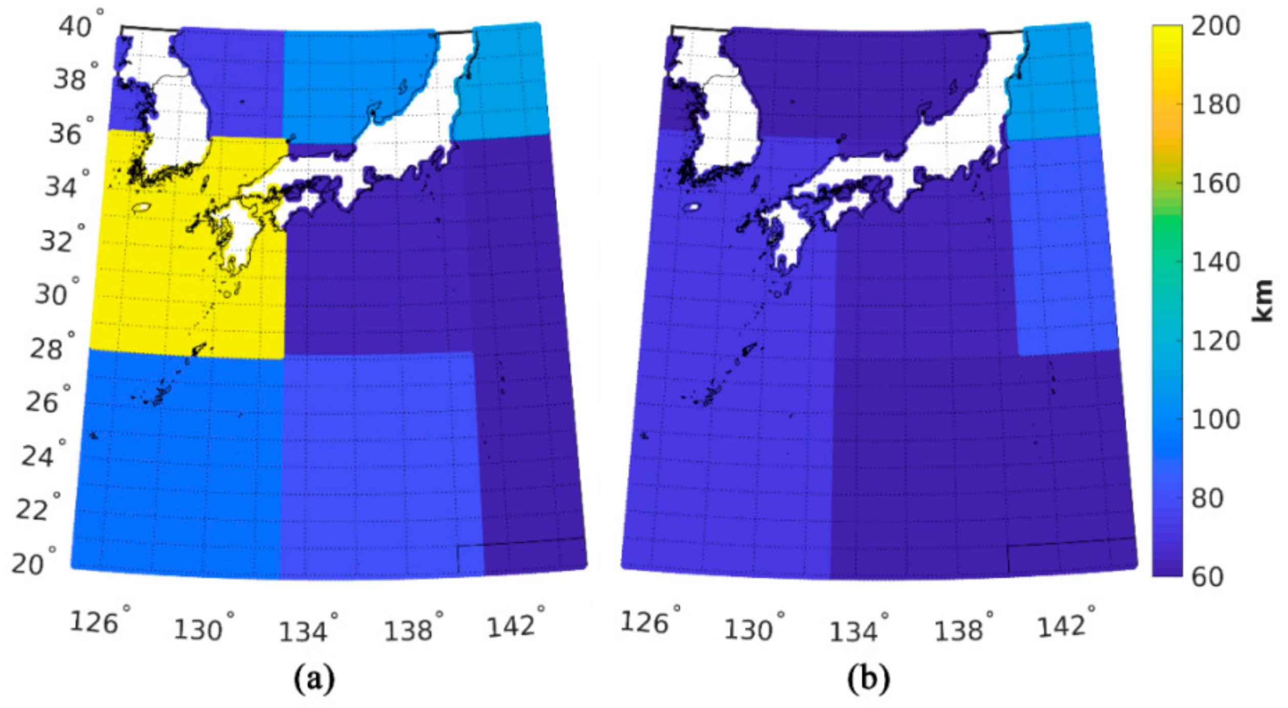
The a priori variance and correlation function of the MDT can be calculated by using the a priori MDT (e.g., CNES-CLS18 MDT). Since the large-scale signal of the MDT was removed in this experiment, only the covariance of the residual part of the MDT needed to be estimated. First, the a priori MDT was Gaussian filtered to obtain the large-scale signals, with the same filter radius as the large-scale MDT. Then, this large-scale MDT was removed from the a priori MDT, and only the variance of the residual part of the MDT signal was calculated and used as the variance of the a priori MDT. In addition, the correlation radius parameter in the covariance function of Equation (8) was the key parameter in the OIM, which refers to the corresponding
and
when the result of the covariance function is zero value and is generally related to the latitude and the ocean basin [
5]. Similarly, the residual part of the MDT could be used for the calculation of the correlation radius in the correlation function: the study area was divided into several subregions, in which the corresponding correlation radius was calculated. It was found that a better MDT solution could be modeled when the subregion was divided into
subregions. In each subregion, the corresponding empirical covariance was calculated based on the distance between the residual MDT grids:
where
is the spherical distance between grids,
is the MDT value of the grid on the spherical surface, and
is the corresponding area. If the subregions are divided by equal areas, this can be simplified to:
where n is the number of the groups of the grids with a spherical distance of
, which could be split by Equation (12):
and fit
as an empirical covariance to a known covariance function (Equation (8)) to determine the correlation radii in zonal and meridional in each region, the results of which are shown in
Figure 3. The sensitivity of the inputs in modeling should be considered [
36]. The sensitivity tests to the covariance of the observations have been analyzed by Rio [
37], and indicated that the correlation scales obtained with different numerical models showed similar patterns. The recently released CNES-CLS18 MDT was used to estimate the variance and correlation function of the MDT in this paper.
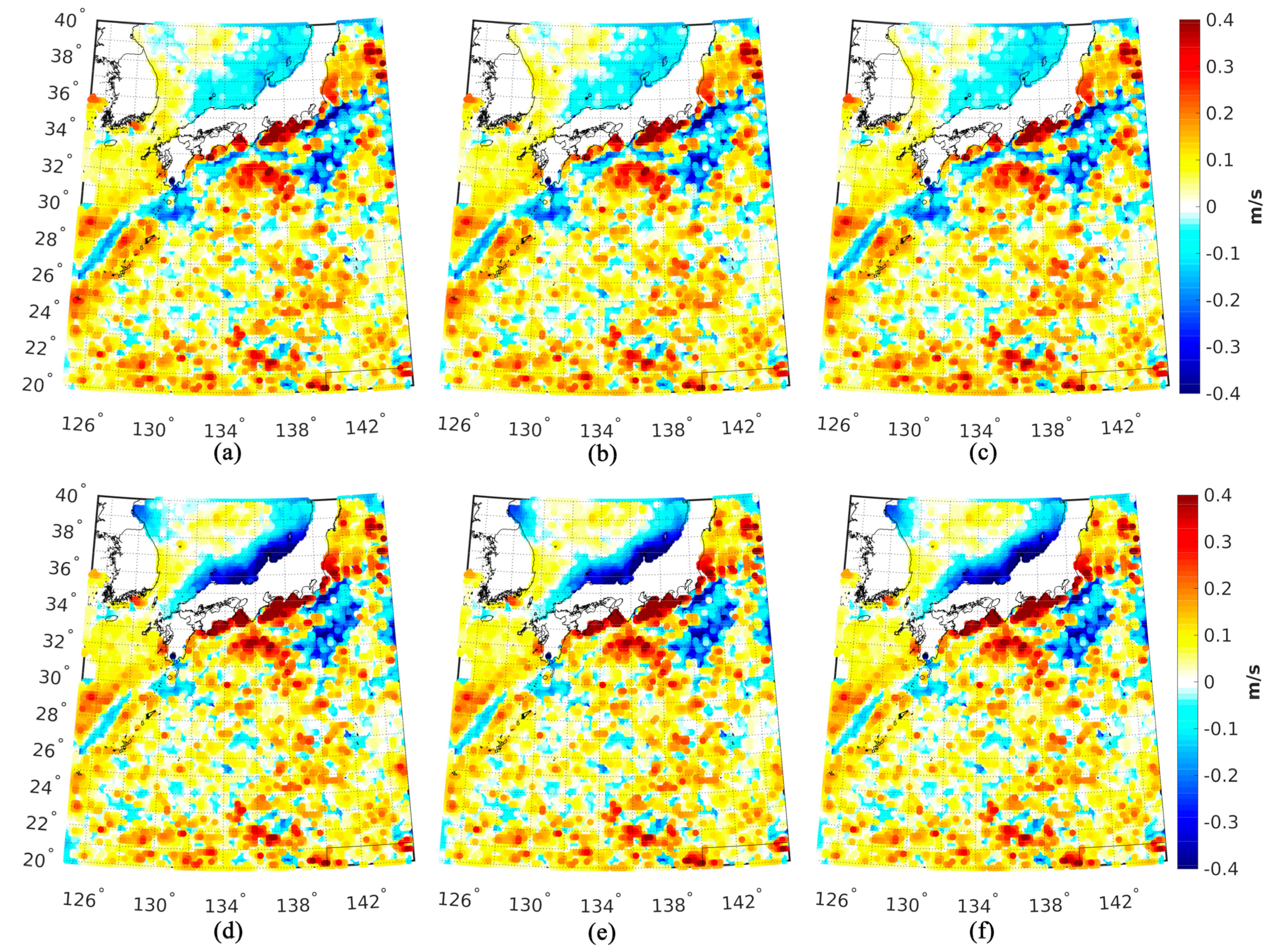
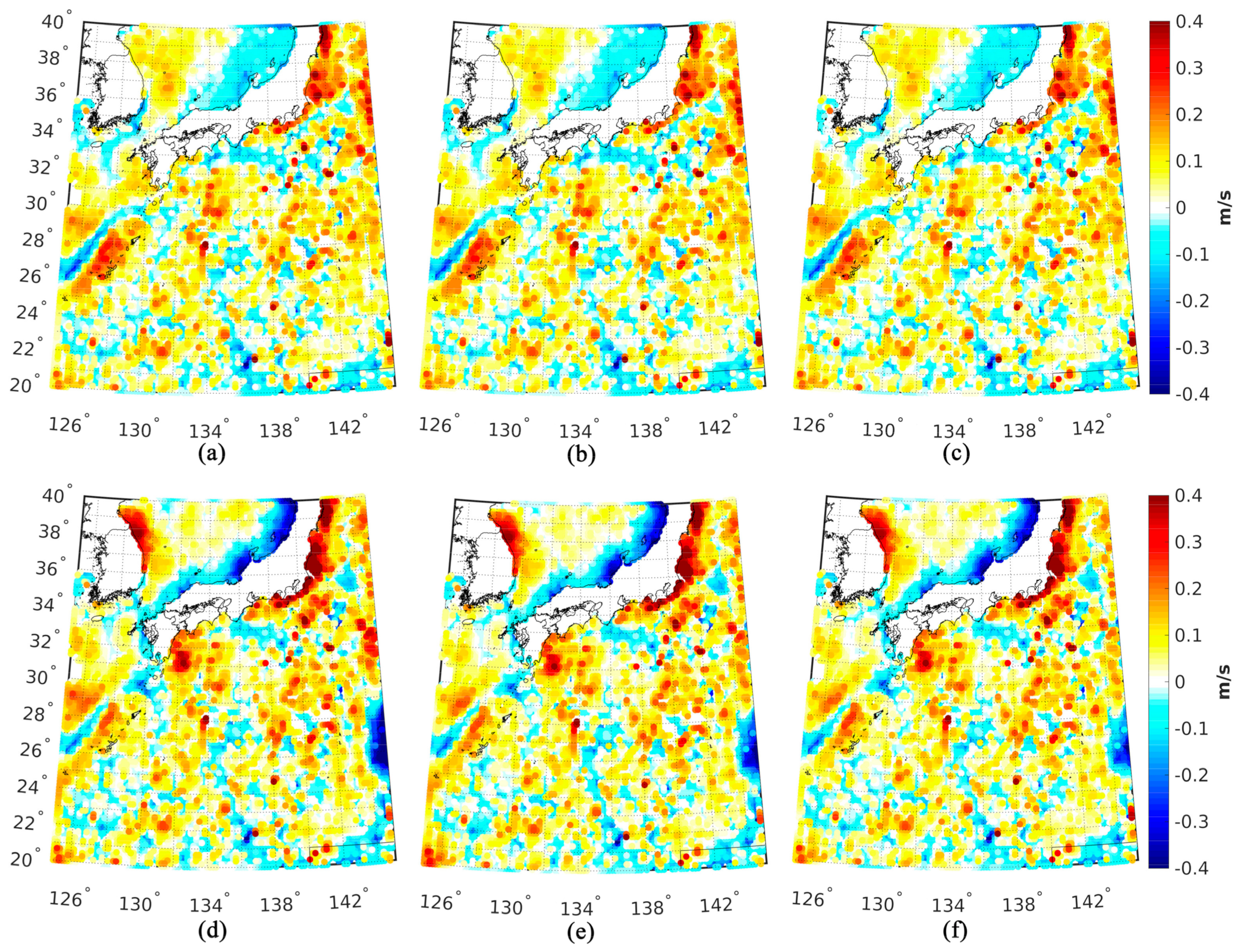
In order to evaluate the performance of the detailed signal recovery of the OIM for the MDT, the geostrophic ocean current velocity could be deduced from the MDT [
38]:
where
and
represent the geostrophic ocean current velocity in the zonal and meridional direction, respectively;
and
represent the latitude and longitude of the point, respectively;
represents the normal gravity,
is the Coriolis force,
is the Earth’s rotation rate, and
is the MDT.


