Smart Topology Optimization Using Adaptive Neighborhood Simulated Annealing

Abstract

Topology optimization (TO) of engineering products is an important design task to maximize performance and efficiency, which can be divided into two main categories of gradient-based and non-gradient-based methods. In recent years, significant attention has been brought to the non-gradient-based methods, mainly because they do not demand access to the derivatives of the objective functions. This property makes them well compatible to the structure of knowledge in the digital design and simulation domains, particularly in Computer Aided Design and Engineering (CAD/CAE) environments. These methods allow for the generation and evaluation of new evolutionary solutions without using the sensitivity information. In this work, a new non-gradient TO methodology using a variation of Simulated Annealing (SA) is presented. This methodology adaptively adjusts newly-generated candidates based on the history of the current solutions and uses the crystallization heuristic to smartly control the convergence of the TO problem. If the changes in the previous solutions of an element and its neighborhood improve the results, the crystallization factor increases the changes in the newly random generated solutions. Otherwise, it decreases the value of changes in the recently generated solutions. This methodology wisely improves the random exploration and convergence of the solutions in TO. In order to study the role of the various parameters in the algorithm, a variety of experiments are conducted and results are analyzed. In multiple case studies, it is shown that the final results are well comparable to the results obtained from the classic gradient-based methods. As an additional feature, a density filter is added to the algorithm to remove discontinuities and gray areas in the final solution resulting in robust outcomes in adjustable resolutions.

1. Introduction

Topology Optimization (TO) is a mathematical method to determine the distribution of material in a design domain in order to maximize the performance of a system [1]. The performance of each system to be optimized includes a wide range of specifications that depend on the application of each system and restrictions. The optimization process could be subjected to some constraints and the final solution must satisfy them. Depending on the TO problem physics, various methodologies have been developed in TO [2,3]. To formulate a TO problem, the design domain is discretized into Finite Elements (FE). The FE should be fine enough to describe the design domain in a reasonable resolution however it should not be too fine that it increase the computational cost without improving the results. The variables are the material density inside each element. Using the intermediate density for elements can improve some common problems: The checkerboard and the discontinuity of the design. The Solid Isotropic Material with Penalization (SIMP) method is one of the most applicable approaches to solving TO problems with less complexity. SIMP models the density of each element with a continuous value between a non-zero minimum and one. This method models the properties of material through a power law approach to penalize unfavorable intermediate densities [4].

The TO algorithm includes generating new solutions and evaluates them based on defined criteria [5]. A variety of methods have been proposed to generate new solutions and evaluate them [2]. From an optimizer point of view, TO methods can be divided into two main types: Gradient-based and non-gradient-based.

The gradient-based methods such as Optimal Criteria (OC) and the Method of Moving Asymptotes (MMA) use sensitivity information of the objective functions (that is, its first order derivatives). In order to obtain the sensitivity information, the derivation of the objective function is required. These methods have a fast convergence to the final results. The gradient-based methods are widely used for TO problems [6,7,8]. Aside from the good performance of these methods in TO, they are limited in the sensitivity information of the objective functions.

However, finding the sensitivity of the objective function is not easy [9]. In such cases, where the objective function derivative is difficult to obtain, the non-gradient-based methods are more advantageous. Non-gradient based methods work only with the value of the objective functions [10,11]. Genetic Algorithm (GA) and Simulated Annealing (SA) are two popular meta-heuristics that have been used in non-gradient-based TO. The main advantage of these non-gradient-based methods is that, unlike gradient-based methods, they do not need the sensitivity information of the objective function.

GA uses the theory of natural selection for heuristic search [12]. Despite GA being used in TO and having represented good results [13], it has high computational costs even for simple problems. The determination of some parameters is also a challenge in GA-based TO which can notably change the results. These parameters are the probability of crossover, probability of mutation, fitness scaling coefficient, population size, selection algorithm, and crossover operator [12].

SA is the other meta-heuristic for non-gradient-based TO. SA uses the concept of metal annealing for the optimization process. The SA generates new candidates randomly and accepts the one which improves the objective function. Additionally, SA also accepts the worst candidates (which do not improve the objective function) under certain conditions [14,15]. This fact allows SA to escape from local minima [16]. The Multi-Resolution Design Variable (MRDV) is used in the literature to enhance search performance [17]. Nevertheless, this approach still has high computational costs and the checkerboard pattern problem still remains. Combining SIMP with SA in structural TO is also used to obtain better results and less gray areas [18]. However, SIMP with SA is not efficient enough due to the high computational costs. Using SA in TO is almost new and needs more research to improve its convergence and computational cost which is the main objective of this work. The proposed algorithm uses the concept of SA with a crystallization factor to improve the performance of TO.

SA with crystallization heuristic controls the probability distribution of the random search [19]. A closed loop is created considering the acceptance or rejection of the new candidate. This closed loop increases the acceptance ratio of new candidates. The SA with crystallization heuristic has been successfully applied in different fields: Cutting and packing [20,21], electrical impedance tomography [22,23,24,25,26,27,28,29,30], curve fitting [31,32,33], etc. The formulation of this method and its application in TO are explained in the next section.

In this paper, the SA with crystallization heuristic has been used for TO as a non-gradient-based method. The two cases of compliance minimization in the classic beam and heat transfer problem have been used to implement this method and verify the results. Analysis of the results has also been done in order to select the input parameters such as the number of iterations and maximum temperature. The problem formulation for the optimization, SA with crystallization heuristic, and TO algorithm will be described in the next section. Then, the results from the proposed method are compared with the results from the literature.

2. Simulated Annealing

The SA is a probabilistic meta-heuristic inspired by the metal annealing process. SA was proposed in the early 80s based on the Metropolis algorithm [14,34,35]. The process starts with an initial solution and in each step, it generates new candidates randomly. The new candidate will be accepted if it improves the objective function or if its Boltzman probability is greater than a random number. The Boltzman probability is calculated by:

$$P\left(T\right)=e^{-\frac{\Delta E}{T}}$$

(1)

where $\Delta E$ is the energy variation, which is the difference between the objective functions for the current solution and the newly generated candidate. T is the current temperature that starts from a high value and decreases in each step until reaching the frozen state. The maximum temperature should be high enough to ensure the domain exploration. Since SA can accept worst candidates, it avoids being stuck in local minima. The generation of new candidates can be performed in different ways. The crystallization heuristic proposed by Martins and Tsuzuki [36] adjusts the probability density to increase the acceptance of new solutions. The SA with crystallization heuristic determines the new candidate $x_{new}$ by:

$$x_{new}=x_{current}+\frac{1}{C_i}\sum _1^{C_i}random(-1/2,1/2)·\Delta r_i·e_i$$

(2)

where $x_{current}$ is the current solution, $\Delta r_i$ is the fixed step size associated with the i-th variable, $e_i$ is the direction of the i-th variable, and $C_i$ is the crystallization factor. Usually, $\Delta r_i=({\max }_i-{\min }_i)/4$ where $[{\min }_i,{\max }_i]$ is the range domain for the i-th variable. The new candidate $x_{new}$ is determined by summing random numbers $C_i$ times (Bates distribution). The crystallization factor $C_i$ varies from 1 and a maximum value. When a new candidate is accepted, the SA considers that it is refining the solution. The SA creates a feedback action which increases exploration, resulting in the reduction of the crystallization factor (this is the negative feedback). On the other hand, when a new candidate is rejected, the SA considers that it is exploring the domain. The SA creates a feedback action which increases refining, resulting in the increase of the crystallization factor (this is the positive feedback).

3. Topology Optimization

Application of TO includes a wide range of problems with different physics. The problems of compliance TO in beams have been used in several research works [6,17,37]. The optimized topologies based on compliance are a good starting point for other TO problems, such as maximum stress, maximum deflection, etc. [3]. Minimizing the compliance of a structure is equal to minimizing the strain energy S which is the external work performed by the external force F with elastic deformation U from an unstressed state as shown in:

$$\begin{array}{cc}\hfill \min & S=U^{T}KU\hfill \\ \hfill \mathrm{Subjected} \mathrm{to}& KU=F\hfill \end{array}.$$

(3)

For a discretized domain with N elements, the density of each element $x_e$ are the TO variables. The total strain energy can be calculated as a strain energy summation in each element with penalized design variable p. According to the SIMP method, it is calculated as:

$$S=\sum _{e=1}^N{\left(x_e\right)}^p{u}_e^T{k}_e{u}_e$$

(4)

where $u_e$ is the element displacement vector and $k_e$ is the element stiffness matrix. The volume fraction constraint determines the final volume regarding the design domain. The optimization process includes the generation of new candidates and objective function evaluation. The SA with crystallization heuristic is used as an optimizer for TO. The algorithm is presented in detail in the next section.

4. SA in TO

In TO with SA meta-heuristic, the optimization starts by assigning an initial random solution and the initial temperature. At each step, a new candidate is generated. The new candidate is the new material density and is calculated according to (2). Then, the objective function is evaluated using FEM with the just determined material density. If the new candidate improves the objective function in comparison with the current solution, the new candidate is directly accepted. Otherwise, the Boltzman probability is calculated using (1). If the Boltzman probability is larger than a random number, the new candidate is accepted.

In both situations, if the new candidate is accepted, the crystallization factor receives negative feedback. It should be noted that the crystallization factor has 1 as the minimum value. In case the new candidate is rejected, the crystallization factor receives positive feedback. The crystallization factor has a maximum value, usually equal to 20 [38,39]. This maximum crystallization factor value ensures a minimum standard deviation value for the probability density distribution. For each temperature, the process of new candidate generation and objective function evaluation is repeated for a predefined number of iterations before going to the next temperature. The SA must reach the thermal equilibrium in the current temperature before going to the next temperature. The thermal equilibrium is reached by evaluating the objective function m times or accepting new candidates $m/2$ times. The value of m must be defined for each TO problem, is usually larger than 40 times the number of variables. A larger m increases the design domain exploration. On the other hand, very large m increases the computational cost, and perhaps less exploration is required. The value of m for each TO must be determined based on the number of elements (variables) and some trial runs. After reaching the thermal equilibrium, the temperature decreases by cooling factor $alpha$. The cooling factor is another parameter to be determined, and a value between $0.8$ and $0.95$ is normally used. The SA converges when the frozen state is reached, this happens when no new candidate is accepted for a specific temperature.

Since this optimization method works based on a probabilistic search, the results come with some discontinuity and gray areas. To reduce discontinuity in borders, a density filter is applied for each element. According to this filter, the density of each element is calculated by:

$$x_{filter}=\frac{{\sum }_{j=1}^{N}w\left(x_j\right)x_j}{{\sum }_{j=1}^{N}w\left(x_j\right)}$$

(5)

based on the weighted density of neighboring elements, where $w\left(x_j\right)$ is the weighting function and represents the distance of neighboring elements subtracted from the filter radius. At higher temperatures, most of the new candidates are accepted as the SA stays in an exploration phase. It is not reasonable to apply the density filter in this situation. The density filter will improve the convergence at lower temperatures, where the SA is already in the refinement phase. The transition from the exploration phase to the refinement phase is not clear. For criteria to start applying the density filter, it considered the situation where $80\%$ or more of rejections happens to be in this transition. After reaching the convergence, a post-processing happens and the density filter is applied again to smoothen the borders and also to turn gray areas into black and white elements.

5. Results

In this section, three study cases are shown. The cantilever and MBB problems in 2D. These two problems allow a comparison of the obtained results with literature results. A practical 3D problem in heat conduction is also shown.

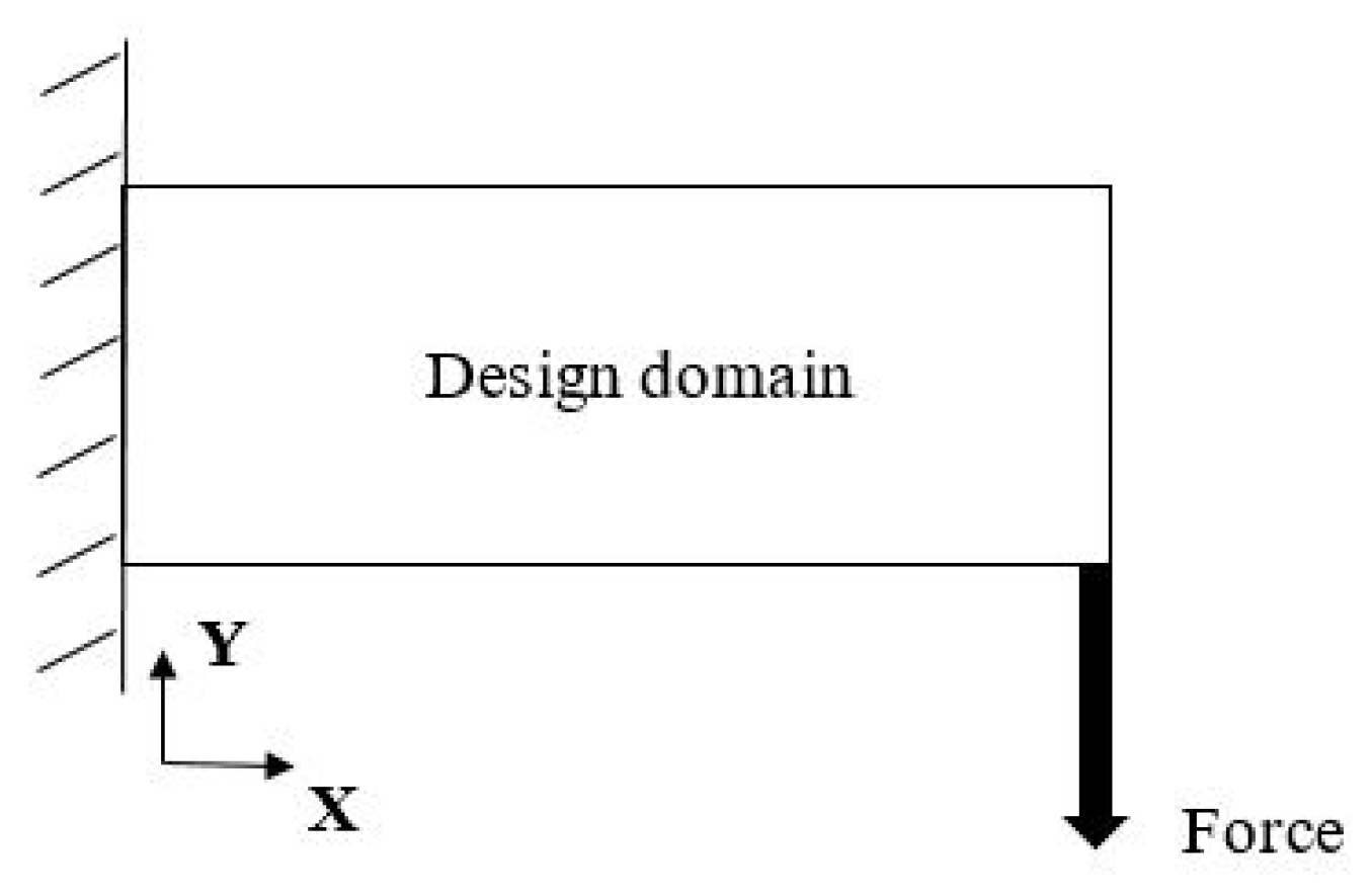
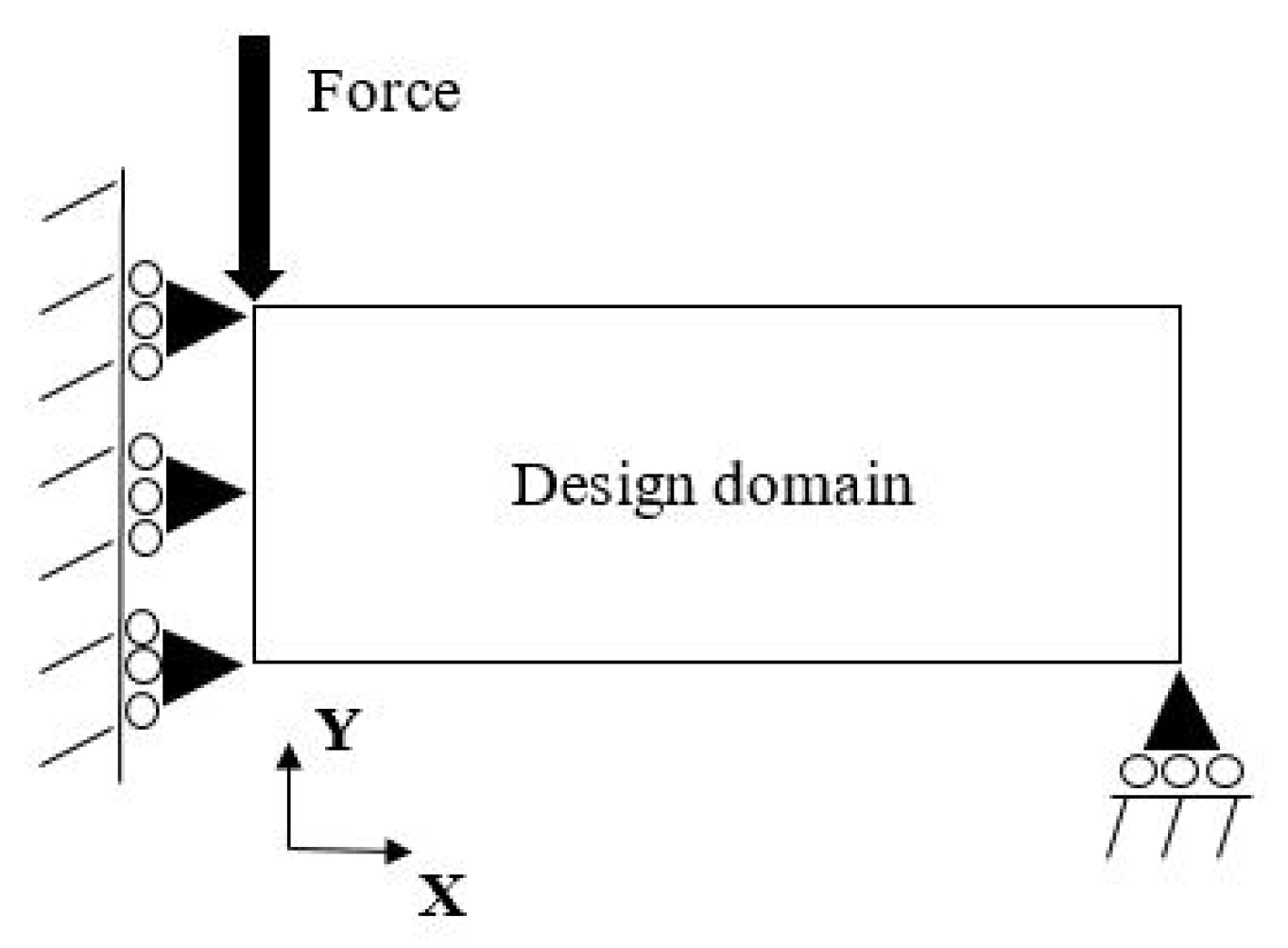
5.1. Cantilever Problem

To verify the proposed method, the classic problem of TO for the cantilever and MBB beam was selected. The cantilever beam is a design domain fixed on one end and a force applied on the other end as shown in Figure 1.

The TO was applied to the cantilever beam with $60\times 30$ elements with a constraint on the volume fraction. The number of elements to discrete the design domain should be high enough to give a good resolution of the final design. In this case, the number of elements was selected based on the similar cases in literature [2]. In other cases, this could be selected simply by considering the minimum required resolution of the final design which depends on the complexity of the expected final design. In order to determine the proper value for m, the optimization process for the cantilever beam problem started with $m=10$. This is a very small value, the motivation was to find a value smaller than $60\times 30\times$ 40 = 72,000, where $30\times 60$ is the number of variables and 40 is the commonly used multiplier. Figure 2 shows the plot of the SA converged objective function value for the optimum solution of a $0.5$-volume fraction versus the value of m.

As shown in Figure 2, the objective function (compliance) starts to converge to the optimum when $m=100$. By increasing the value of m until 1000, the converged objective function value will not have any considerable changes and it is already very close to the optimum solution. Similarly, for other volume fractions, the convergence has the same behavior. Since the computational cost for this problem is not too high, $m=1000$ was used in the simulations. In more complicated problems, a reasonable value of m can be determined using a similar approach.

The frozen state is defined as the temperature where no new candidate is accepted. It is necessary to determine the initial temperature value. In an attempt to stop the SA before reaching the frozen state and to define the initial temperature, the following study was executed. The number of rejected and accepted new candidates per temperature were computed. It resulted in the graph shown in Figure 3. In the SA, the number of accepted solutions must be as high as possible in the exploration phase. From Figure 3, at a temperature near 100, SA has an acceptance ratio of about $60\%$. The initial temperature $T_0=100$ is reasonable, and allows the SA to have enough domain exploration. The final temperature was selected as $T_{end}=0.001$ in which the number of accepted solutions is already small. The real frozen state cannot be reached, because of the checker board problem.

The problem of minimizing compliance in the cantilever beam of Figure 1 is solved with the gradient-based method from the literature [6] and the method proposed herein. The results are presented in

Table 1. Cantilever beam compliance for different volume fractions from the literature and the method proposed herein.

Volume Fraction	Compliance from [6]	Compliance from the Method Proposed Herein
0.5	70.41	73.71
0.6	60.43	61.42
0.7	53.95	54.97
0.8	49.68	50.21
0.9	46.84	47.10

for different volume fractions. The parameters used for the SA in the proposed method are $T_0=100$ and $T_{end}=0.001$ for initial and final temperatures, $m=1000$ to reach the thermal equilibrium, and $\alpha =0.85$ for the cooling factor.

The compliance of optimized cantilever beam using the proposed method agrees very well with the values from the literature. Figure 4 shows the optimized topology of cantilever beam for different volume fractions. The shapes from the method proposed herein are similar to the results from the literature.

Each variable has its crystallization factor and their value shows the crystallization of the variable as the temperature decreases. The value of the crystallization factor indicates if the variable is in an exploratory or refinement phase. Crystallization factors with higher values indicate that the variables are in the refinement phase. Crystallization factors with smaller values indicate that the variables are in the exploration phase. Four different variables were selected as shown in Figure 5a. The graph average of the crystallization factors for the four points per temperature is presented in Figure 5b.

As shown in Figure 5, the variable C1 started randomly as void or solid, its crystallization factor is shown in blue and it quickly reaches the maximum value. C3 is another variable, its crystallization factor is shown in yellow. It takes more iterations to get to the frozen state. Near the temperature of $0.01$, all four crystallization factors associated with the four selected variables reach the frozen state (its maximum value).

5.2. MBB Problem

The second studied problem is the Messerschmitt–Bolkow–Blohm (MBB) beam. The design domain is a simply supported beam with a vertical force in the middle. Since the design domain is symmetric, half of it considered here as showed in Figure 6. Since the design domain is completely symmetric, only half of the design domain is considered in TO. A similar procedure, as described for the previous example (see Figure 6), was performed to determine the value of m. The graph shown in Figure 7 shows the graph of the converged objective function value versus the value of m.

As shown in Figure 7, with more than $m=100$, the converged objective function value is near the optimum. It can be noticed from Figure 2 and Figure 7 that the minimum required value of m depends on the number of variables, and it is almost independent of the loading and boundary conditions. The same input parameters of the cantilever beam problem are used to solve the half-MBB TO problem in Figure 6. The results for the compliance of optimized topology in different volume fractions are presented in

Table 2. Half-MBB beam compliance for different volume fractions from the literature and the proposed method.

Volume Fraction	Compliance from [6]	Compliance from the Method Proposed Herein
0.5	77.42	80.87
0.6	66.73	68.55
0.7	59.69	60.72
0.8	54.55	55.60
0.9	51.31	51.95

. The results for the half-MBB problem also agrees very well with the results from the literature. The final shape for the half-MBB problem is shown in Figure 8.

5.3. Heat Conduction Problem

The results for the TO of the cantilever and half-MBB beam shows that the proposed method is as efficient as the gradient-based TO methods. It should be noted that the main significance of the proposed method is the inclusion of sensitivity information without using any gradient information. Since this method works based on a probabilistic search, the final shapes are not as smooth as the other methods. However, the use of finer mesh or the application of some post processing can improve the final results.

In order to show the usefulness of this method in practical problems, a 3D heat conduction problem was also studied. The schematic of the design domain is shown in Figure 9. In the heat transfer problem, the heat sink is at a different temperature and the heat flows throw the design domain. The formulation of the heat transfer in the FE format is similar to (3). The difference is that in the heat transfer problem U is the finite global nodal temperature vector, F is the global thermal load vector, and K is the global thermal conductivity. The thermal conductivity matrix or stiffness matrix for the heat conduction problem can be obtained by the assembly of element thermal conductivity matrices. The SIMP method gives the thermal conductivity matrix of each element by interpolating the density of each element. The design domain in Figure 9 is in 3D and all the nodes and matrices should be in 3D as well. For isotropic material, the thermal properties are equal in all directions. The objective function of this heat conduction problem to be minimized is the heat transfer compliance.

According to the literature [8], a $40\times 40$ element in x and y directions can define the problem efficiently. To ease the results comparison, just one element is considered in the z direction. To determine the proper number of iterations, the optimization process has been performed with different values of m and the results are shown in Figure 10. From Figure 10, the converged objective function approximated the optimum solution for values of m greater than 300. The higher the m, the slightly better the results will be, and since the computational costs are low, the value of $m=5000$ was chosen. The final optimum solution values of heat transfer compliance from the literature [8] and the proposed method are presented in

Table 3. Minimized heat transfer compliance for different volume fractions from the literature and the method proposed herein.

Volume Fraction	Compliance from [8]	Compliance from the Proposed Method
0.5	250.75	224.56
0.6	211.83	196.44
0.7	189.88	182.27
0.8	180.18	173.51
0.9	170.89	169.11

.

The final shape of optimized topologies from the literature [8] and the proposed method are presented in Figure 11 for a $40\times 40\times 1$ element design domain.

As shown in Figure 11 and Table 3, the results from the proposed method and the literature for the heat transfer problem are almost the same. The value of the minimum compliance has also slightly improved.

6. Conclusions

A new method for TO of mechanical structures is proposed in this work. The proposed method uses the concept of SA with crystallization heuristic to determine the optimal shape. The crystallization heuristic improved the search in the generation of the new candidate. Although this algorithm is non-gradient based and derivatives of the objective functions are not required, the algorithm uses a feedback action, depending on whether the new candidate is accepted or rejected, the crystallization factor is modified accordingly. A density filter is also applied when the thermal equilibrium is reached to smoothen the borders. Applying the proposed method to the classic problem of compliance minimization in the cantilever beam and MBB beam showed good agreement with the results from the literature. Similarly, the proposed method for the problem of minimizing heat transfer compliance showed good agreement with results from the literature. It shows that this method can be used for any type of problem regardless of the existence of sensitivity information.

Since this method is new, a considerable amount of research and developments are required to improve and prepare it for commercial use. Future work could reduce the computational costs by the calculation of the objective function in different ways. This method could also be applied to multi-objective TO problems.

References

1. Marchesi, T.R.; Lahuerta, R.D.; Silva, E.C.N.; Tsuzuki, M.S.G.; Martins, T.C.; Barari, A.; Wood, I. Topologically optimized diesel engine support manufactured with additive manufacturing. IFAC-PapersOnLine 2015, 28, 2333–2338. [Google Scholar] [CrossRef]
2. Sigmund, O.; Maute, K. Topology optimization approaches. Struct. Multidiscip. Optim. 2013, 48, 1031–1055. [Google Scholar] [CrossRef]
3. Bendsoe, M.P.; Sigmund, O. Topology Optimization: Theory, Methods, and Applications; Springer Science & Business Media: Berlin/Heidelberg, Germany, 2013. [Google Scholar]
4. Rozvany, G. The SIMP method in topology optimization-theoretical background, advantages and new applications. In Proceedings of the 8th Symposium on Multidisciplinary Analysis and Optimization, Long Beach, CA, USA, 6–8 September 2000; p. 4738. [Google Scholar]
5. Huang, X.; Xie, M. Evolutionary Topology Optimization of Continuum Structures: Methods and Applications; John Wiley & Sons: Hoboken, NJ, USA, 2010. [Google Scholar]
6. Sigmund, O. A 99 line topology optimization code written in Matlab. Struct. Multidiscip. Optim. 2001, 21, 120–127. [Google Scholar] [CrossRef]
7. Andreassen, E.; Clausen, A.; Schevenels, M.; Lazarov, B.S.; Sigmund, O. Efficient topology optimization in MATLAB using 88 lines of code. Struct. Multidiscip. Optim. 2011, 43, 1–16. [Google Scholar] [CrossRef] [Green Version]
8. Liu, K.; Tovar, A. An efficient 3D topology optimization code written in Matlab. Struct. Multidiscip. Optim. 2014, 50, 1175–1196. [Google Scholar] [CrossRef] [Green Version]
9. Jankovics, D.; Gohari, H.; Tayefeh, M.; Barari, A. Developing topology optimization with additive manufacturing constraints in ANSYS®. IFAC-PapersOnLine 2018, 51, 1359–1364. [Google Scholar] [CrossRef]
10. Sigmund, O. On the usefulness of non-gradient approaches in topology optimization. Struct. Multidiscip. Optim. 2011, 43, 589–596. [Google Scholar] [CrossRef]
11. Munk, D.J.; Vio, G.A.; Steven, G.P. Topology and shape optimization methods using evolutionary algorithms: A review. Struct. Multidiscip. Optim. 2015, 52, 613–631. [Google Scholar] [CrossRef]
12. Chapman, C.D. Structural Topology Optimization via the Genetic Algorithm. Ph.D. Thesis, Massachusetts Institute of Technology, Cambridge, MA, USA, 1994. [Google Scholar]
13. Hajela, P.; Lee, E.; Lin, C.Y. Genetic algorithms in structural topology optimization. In Topology Design of Structures; Springer: Berlin/Heidelberg, Germany, 1993; pp. 117–133. [Google Scholar]
14. Kirkpatrick, S.; Gelatt, C.D.; Vecchi, M.P. Optimization by simulated annealing. Science 1983, 220, 671–680. [Google Scholar] [CrossRef] [PubMed]
15. Rutenbar, R.A. Simulated annealing algorithms: An overview. IEEE Circuits Devices Mag. 1989, 5, 19–26. [Google Scholar] [CrossRef]
16. Najafabadi, H.R.; Goto, T.G.; Martins, T.C.; Barari, A.; Tsuzuki, M.S. Multi-objective topology optimization using simulated annealing method. In Proceedings of the International Conference on Geometry and Graphics, São Paulo, Brazil, 18–22 January 2021; pp. 343–353. [Google Scholar]
17. Bureerat, S.; Limtragool, J. Structural topology optimisation using simulated annealing with multiresolution design variables. Finite Elem. Anal. Des. 2008, 44, 738–747. [Google Scholar] [CrossRef]
18. Garcia-Lopez, N.; Sanchez-Silva, M.; Medaglia, A.; Chateauneuf, A. A hybrid topology optimization methodology combining simulated annealing and SIMP. Comput. Struct. 2011, 89, 1512–1522. [Google Scholar] [CrossRef]
19. Martins, T.C.; Tsuzuki, M.S.G. Rotational placement of irregular polygons over containers with fixed dimensions using simulated annealing and no-fit polygons. J. Braz. Soc. Mech. Sci. 2008, 30, 205–212. [Google Scholar] [CrossRef] [Green Version]
20. Martins, T.C.; Tsuzuki, M.S.G. Simulated annealing applied to the rotational polygon packing. IFAC (IFAC-PapersOnline) 2006, 12, 475–480. [Google Scholar]
21. Sato, A.K.; Martins, T.C.; Tsuzuki, M.S.G. Rotational placement using simulated annealing and collision free region. IFAC Proc. Vol. 2010, 43, 234–239. [Google Scholar] [CrossRef]
22. Martins, T.C.; Camargo, E.D.L.B.; Lima, R.G.; Amato, M.B.P.; Tsuzuki, M.S.G. Electrical impedance tomography reconstruction through Simulated Annealing with incomplete evaluation of the objective function. In Proceedings of the 33rd IEEE EMBC, Boston, MA, USA, 30 August–1 September 2011; pp. 7033–7036. [Google Scholar]
23. Martins, T.C.; Tsuzuki, M.S.G. Simulated annealing with partial evaluation of objective function applied to electrical impedance tomography. IFAC Proc. Vol. 2011, 44, 4989–4994. [Google Scholar] [CrossRef] [Green Version]
24. Tavares, R.S.; Martins, T.C.; Tsuzuki, M.S.G. Electrical impedance tomography reconstruction through aimulated annealing using a new outside-in heuristic and GPU parallelization. J. Physics: Conf. Ser. 2012, 407, 012015. [Google Scholar]
25. Martins, T.C.; Tsuzuki, M.S.G. Electrical impedance tomography reconstruction through simulated annealing with total least square error as objective function. In Proceedings of the 34th IEEE EMBC, San Diego, CA, USA, 28 August 28–1 September 2012; pp. 1518–1521. [Google Scholar]
26. Martins, T.C.; Tsuzuki, M.S.G. Electrical impedance tomography reconstruction through simulated annealing with multi-stage partially evaluated objective functions. In Proceedings of the 35th IEEE EMBC, Osaka, Japan, 3–7 July 2013; pp. 6425–6428. [Google Scholar]
27. Martins, T.C.; Fernandes, A.V.; Tsuzuki, M.S.G. Image reconstruction by electrical impedance tomography using multi-objective simulated annealing. In Proceedings of the IEEE 11th ISBI, Beijing, China, 29 April–2 May 2014; pp. 185–188. [Google Scholar]
28. Martins, T.C.; Tsuzuki, M.S.G. EIT image regularization by a new multi-objective simulated annealing algorithm. In Proceedings of the 37th IEEE EMBC, Milano, Italy, 25–29 August 2015; pp. 4069–4072. [Google Scholar]
29. Martins, T.C.; Tsuzuki, M.S.G.; Camargo, E.D.L.B.D.; Lima, R.G.; Moura, F.S.D.; Amato, M.B.P. Interval simulated annealing applied to electrical impedance tomography image reconstruction with fast objective function evaluation. Comput. Math Appl. 2016, 72, 1230–1243. [Google Scholar] [CrossRef]
30. Martins, T.C.; Tsuzuki, M.S.G. Investigating anisotropic EIT with simulated annealing. IFAC-PapersOnLine 2017, 50, 9961–9966. [Google Scholar] [CrossRef]
31. Ueda, E.K.; Tsuzuki, M.S.G.; Takimoto, R.Y.; Sato, A.K.; Martins, T.C.; Miyagi, P.E.; Rosso, R.S.U., Jr. Piecewise Bézier curve fitting by multiobjective simulated annealing. IFAC-PapersOnLine 2016, 49, 49–54. [Google Scholar] [CrossRef]
32. Ueda, E.K.; Tsuzuki, M.S.; Barari, A. Piecewise Bézier curve fitting of a point cloud boundary by simulated annealing. In Proceedings of the 2018 13th IEEE International Conference on Industry Applications (INDUSCON), Sao Paulo, Brazil, 12–14 November 2019; pp. 1335–1340. [Google Scholar]
33. Ueda, E.K.; Barari, A.; Sato, A.K.; Tsuzuki, M.S.G. Detection of defected zone using 3D scanning data to repair worn turbine blades. In Proceedings of the 21st IFAC World Congress, Berlin, Germany, 12–17 July 2020; pp. 10666–10670. [Google Scholar]
34. Černý, V. Thermodynamical approach to the traveling salesman problem: An efficient simulation algorithm. J. Optim. Theory Appl. 1985, 45, 41–51. [Google Scholar] [CrossRef]
35. Metropolis, N.; Rosenbluth, A.W.; Rosenbluth, M.N.; Teller, A.H.; Teller, E. Equation of state calculations by fast computing machines. J. Chem. Phys. 1953, 21, 1087–1092. [Google Scholar] [CrossRef] [Green Version]
36. Martins, T.C.; Tsuzuki, M.S.G. Placement over containers with fixed dimensions solved with adaptive neighborhood simulated annealing. Pol. Acad. Sci. Tech. 2009, 57, 273–280. [Google Scholar] [CrossRef] [Green Version]
37. Deng, S.; Suresh, K. Multi-constrained topology optimization via the topological sensitivity. Struct. Multidiscip. Optim. 2015, 51, 987–1001. [Google Scholar] [CrossRef]
38. Ueda, E.K.; Sato, A.K.; Martins, T.C.; Takimoto, R.Y.; Rosso, R.S.U., Jr.; Tsuzuki, M.S.G. Curve approximation by adaptive neighborhood simulated annealing and piecewise Bézier curves. Soft Comput. 2020, 24, 18821–18839. [Google Scholar] [CrossRef]
39. Tavares, R.S.; Sato, A.K.; Martins, T.C.; Lima, R.G.; Tsuzuki, M.S.G. GPU acceleration of absolute EIT image reconstruction using simulated annealing. Biomed. Signal. Process. Control 2019, 52, 445–455. [Google Scholar] [CrossRef]
Figure 1. Schematic of design domain and loading condition for cantilever beam.
Applsci 11 05257 g001
Figure 2. SA converged objective function value versus value of m for the cantilever beam problem with volume fraction 0.5 (m is the number of objective function evaluations to reach thermal equilibrium in a specific temperature).
Applsci 11 05257 g002
Figure 3. Number of accepted and rejected new candidates versus temperature. This graph shows that a reasonable initial temperature is T 0 = 100 where 60 % of the new candidates are accepted.
Applsci 11 05257 g003
Figure 4. The results for optimized topology of cantilever beam in different volume fractions of 0.5, 0.6, 0.7, 0.8, and 0.9. (a) Results from the literature. (b) Results from the method proposed herein.
Applsci 11 05257 g004
Figure 5. (a) Four arbitrary variables in the design domain of the cantilever beam were selected. (b) The average crystallization factor for each of these variables per temperature is plotted.
Applsci 11 05257 g005
Figure 6. Schematic of design domain and loading condition for the half-MBB beam.
Applsci 11 05257 g006
Figure 7. SA converged objective function value versus value of m for the MBB beam problem with a 0.5-volume fraction (m is the number of objective function evaluations to reach thermal equilibrium in a specific temperature).
Applsci 11 05257 g007
Figure 8. The results for optimized topology of a half-MBB beam in different volume fractions of 0.5, 0.6, 0.7, 0.8, and 0.9. (a) Results from the literature. (b) Results from the proposed method.
Applsci 11 05257 g008
Figure 9. Schematic of the design domain for the heat conduction problem.
Applsci 11 05257 g009
Figure 10. SA converged objective function value versus value of m for the heat conduction problem with a 0.5-volume fraction (m is the number of objective function evaluations to reach thermal equilibrium in a specific temperature).
Applsci 11 05257 g010
Figure 11. The results for optimized topology of heat conduction in different volume fractions of 0.5, 0.6, 0.7, 0.8, and 0.9.(a) Results from the literature. (b) Results from the proposed method.
Applsci 11 05257 g011