Evaluation of the Water Shielding Performance of a Capillary Barrier System through a Small-Scale Model Test

Abstract

Capillary barrier (CB) systems consisting of a fine-grained soil layer placed over a coarse-grained soil layer can generally provide a water-shielding effect, increasing the slope stability of soil structures during rainfall. In order to improve the water-shielding performance of CB systems, laboratory model tests have been previously conducted under various conditions; notably, large-scale model tests are especially required. The inefficiency in increasing the production time of CB models until now explains their high cost. In this paper, we propose a laboratory small-scale CB (SSCB) model test for a quick and efficient evaluation of the function of a CB system. In this model test, differently from previous studies, a side drainage flow in the direction of the inclined sand layer was set as the no-flow condition; moreover, the laboratory SSCB model tests were performed by considering three rainfall intensities (i.e., 20, 50, and 100 mm/h) under the lateral no-flow condition. The results showed that the larger the rainfall intensity, the shorter the diversion length was of the CB system. To evaluate the effectiveness of the SSCB model test proposed in this study, the diversion length was estimated by an empirical equation under the lateral flow condition based on hydraulic conductivity functions and the soil water characteristic curves of sand and gravel and then compared to the results of the SSCB model tests. It was hence demonstrated that the water-shielding performance of the CB system can be efficiently evaluated through SSCB model tests under the lateral no-flow condition, rather than through large-scale model tests.

1. Introduction

Capillary barrier (CB) systems, consisting of a layer of fine-grained material (e.g., silty or sandy soil) over one of coarse soil (e.g., gravel), provides a water-shielding effect, minimizing rainfall infiltration into the soil structure [1]. One of the advantages of the CB system is that it is eco-friendly because it generally consists exclusively of natural materials (e.g., silt, sand, and gravel). This system has been applied as a landfill cover system for waste disposal sites or as an oxygen barrier to limit the production of acid mine drainage: it allows a safe discharge of rainwater infiltrated from the surface to the outside [2,3,4,5,6,7,8]. Moreover, the CB system has been used as a final capping system after the closure of nuclear waste facilities [9]. Some researchers have also considered the application of the CB system for the maintenance of slope stability in soil structures since it can prevent rainwater infiltration into engineered slopes [10,11,12,13,14,15,16,17,18,19]. Meanwhile, many laboratory CB model tests have been performed to examine and improve the water-shielding performance of the CB system under the influence of several factors (e.g., material properties and layer thickness) [15,20,21,22,23,24]. Numerical simulations associated with the design of a physical CB model have been also carried out under diverse conditions [16,25,26,27].

For example, Bussière et al. [26] performed laboratory CB model tests using a rectangular box (3.0 m long, 1.5 m high, and 1.0 m wide) to evaluate the slope effects on the hydraulic behavior of a CB. They reported that the slope influenced water distribution in the layers. Based on the results of numerical modeling, they also showed that the geometry of the CB model is one of the key issues to be considered to properly analyze the behavior of CBs used for controlling water infiltration [9]. Ng et al. [21] proposed a three-layer CB landfill cover system for minimizing rainfall infiltration in humid climates. To evaluate the effectiveness of the new system, they used a flume model (3.0 m long, 1.5 m high, and 1.0 m wide). Their experimental and back-analysis results indicated that no water seeped through the tested three-layer barrier. Zhan et al. [22] performed laboratory CB model tests to observe the response of a three-layer CB system under a continuous heavy rainfall of 70 mm/h. Their inclined model box was 2.0 m long, 1.0 m high, and 1.2 m wide. The authors reported that the three-layer CB system did not allow deep percolation under heavy rainfall; moreover, the correlation between the physical and numerical modeling results indicated an anisotropic behavior of the system with respect to hydraulic conductivity in the unsaturated sand layer. Matsumoto et al. [23] considered the use of a three-layer barrier for improving the water-shielding performance of the CB system. They hence performed a series of laboratory CB model tests using a large-scale model box (3.0 m long, 1.5 m high, and 1.0 m wide). The effect of each layer’s thickness change on the system function was investigated. It was hence found that the measured results and those estimated through the empirical equation of Steenhuis et al. [28] (for upper (silica sand No. 6) and middle (silica sand No. 8) layers with thicknesses of ≥ 50 cm and ≥ 30–50 cm, respectively) were similar.

In the laboratory CB model tests of those mentioned above, a large-scale model with a lateral length ≥ 2.0 m was used: in this case, the water infiltration from the upper sand layer to the lower gravel layer occurred randomly. This large-scale model test requires a lot of time for its functioning; moreover, its fabrication is expensive, and the corresponding testing time is high, making it difficult to perform many CB model tests under different conditions. Additional methodologies such as the BoSG (Boolean Stochastic Generation) and the Monte Carlo technique to characterize the infiltration and geomechanical parameters by means of random approaches in the numerical modeling for the slope stability may be needed [29,30,31]. Thus, in this paper, we propose a laboratory small-scale CB (SSCB) model test that can quickly and efficiently evaluate the water-shielding performance of a CB system. Differently from previous studies, here the SSCB system was characterized by setting the drainage condition in the flow direction of the inclined sand layer as the lateral no-flow (i.e., undrained) condition. This testing condition induced a quick infiltration of the water contained in the sand layer into the gravel layer in the flow direction, while the infiltrated water was drained from the gravel layer to the outside. Thus, the drainage condition of the SSCB model test reproduced an extreme condition for the CB system, which would result from the infiltration of rainfall from the surface layer. It is hence expected that the size of the CB model tests can be reduced and that their manufacturing time and corresponding testing time can be shortened. To examine the effectiveness of the proposed SSCB model test under the lateral no-flow condition of the inclined sand layer, we performed multiple tests by considering three different rainfall intensities (i.e., 20, 50, and 100 mm/h). Water retention tests were also carried out to obtain the soil-water characteristic curves of the sand and gravel used in this study. The diversion lengths that represent the water-shielding performance of the CB were estimated by the empirical equation of Steenhuis et al. [28] under the lateral flow (i.e., drained) condition, based on the physical and water retention characteristics of the sand and gravel. Comparing the results of the SSCB model test with the values estimated by the empirical equation, we finally discussed the significance and validity of the laboratory SSCB model test under the lateral no-flow condition.

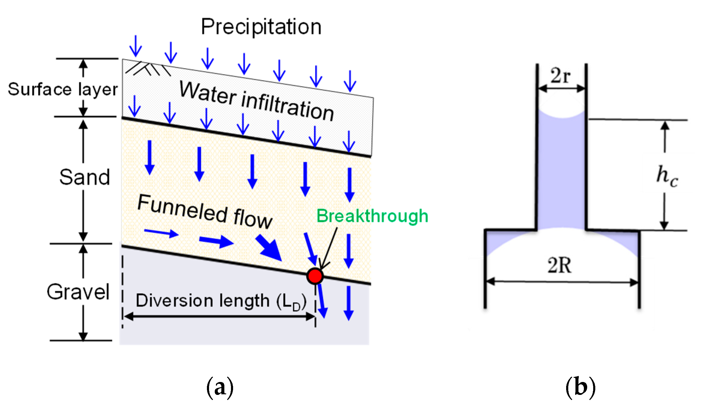
2. Characteristic of the CB System

In the stratified grounds, where a sand layer can naturally occur over a gravel layer, infiltrated water tends to be retained and to accumulate in the sand above the contact interface, due to the different water retention characteristics of the two types of layers (Figure 1) [1]. The interface between the sand and gravel layers, which acts as a wall (preventing the infiltration of water from the sand layer into the gravel layer), can be identified as a CB. Since the CB is capable of protecting certain areas of the interface below the sand layer from water infiltration, this type of barrier has been widely used in soil structures, such as burial mounds and reservoirs. The functioning of CBs is based on a continuous capillary mechanism, which involves soil layers with different thicknesses. In Figure 1b, the relatively thin capillary tube at the top (with diameter r) represents the void formed in the upper layer (made of fine-grained soil), while the relatively thick capillary tube at the bottom (with diameter 2R) represents the void formed in the lower layer (made of coarse-grained soil). The water droplets that flow in the unsaturated state are maintained by the capillary force just above the junction of the thin and thick capillary tubes [32]. The height (h_c) of the water column, which is maintained in an equilibrium state, can be expressed by the following equation:

$$h_c=\frac{2T}{{\rho }_{w}g}(\frac{1}{r}-\frac{1}{R})$$

(1)

where r and R are the radiuses of the upper thin and lower thick capillary tubes, respectively, T (0.074 N/m in water at 15 °C) is the surface tension of water, ρ_w is the density of water, and g is the acceleration of gravity. Since r is always smaller than R, the larger the difference in size between the particle diameters of the fine and coarse soils, the more moisture will be maintained by the fine-grained soil layer containing the upper fine capillary tube.

CB systems systematically used in geotechnical engineering can also be composed of a fine soil (i.e., sand) layer over a coarse soil (i.e., gravel) layer, as shown in Figure 1. Since natural soils can be used for the creation of CB systems, such systems are eco-friendly. The water-shielding performance of a CB system is usually determined by the difference in hydraulic conductivity functions and soil-water characteristic curves between the sand and the gravel used for its creation [33]. In particular, the difference in the relative water retention of soil in the unsaturated condition can be understood by studying the soil-water characteristic curve (SWCC) [34]. As explained above, because the water-retaining capacity of sand is relatively larger than that of gravel, water retained in the upper sand layer tends to flow along the interface between the sand and gravel layers and to accumulate in the bottom part of the sand layer. This generates a funneled flow in an inclined direction (Figure 1). However, as the degree of saturation of the sand layer increases due to continuous water infiltration at the top of the interface, the difference in water retention between sand and gravel gradually decreases. Specifically, as the suction of the sand layer decreases, the unsaturated hydraulic conductivities (k_w) of the two samples become the same [12,35,36,37,38]. At this point, water begins to infiltrate the lower gravel layer (i.e., the “breakthrough” phase), and the CB system finally loses its water-shielding performance.

The above processes can be understood as a water retention function of the CB, or as a water-shielding performance that results in the retention of water in the upper layer and suppresses water infiltration to the lower layer. For improving the CB’s function, it is necessary to determine the contrast between coarse particles and fine grains, make sure to always maintain the soil around the CB in an unsaturated state, and reduce the amount of water infiltrating from the surface layer [32,39,40]. The horizontal distance from the top of the slope to the breakthrough point is defined as the diversion length (L_D) of the CB system (i.e., an indicator of its water-shielding performance) (see Figure 1) [41].

When applying the CB system to water-shielding or to the control of infiltrated water, L_D is an important design parameter, which determines the size and structure of the CB system. The size of L_D is related to the slope angle of the interface (as a structural factor), to the water retention characteristics of sand and gravel (as a material factor), and to the infiltration rate (as an external factor). Empirical equations for estimating the diversion length under the lateral flow (i.e., drained) condition and considering these influencing factors have been proposed by Ross [4], Kung [42], and Steenhuis et al. [28]. Among these, the equation of Steenhuis et al. [28], based on Kung’s equation, is considered to have a particularly good accuracy [43,44]. In this study, we compared the relationship between the estimated and measured L_D values. First, the estimated values explained later were derived using Equation (2) proposed by Steenhuis et al. [28], based on modified Kung’s equation. It should be noted that in this equation, the layer thickness does not affect the diversion length:

$${\mathrm{L}}_{\mathrm{D}}=\tan \Phi \cdot \{\frac{1}{b}(\frac{1}{\kappa }-1)+\frac{1}{\kappa }(h_{ae}-h_{ex})\}$$

(2)

where b was derived from the equation of unsaturated hydraulic conductivity and from the relationship k = k_sat·exp(bψ_m) (with k_sat being the saturated hydraulic conductivity and ψ_m the suction (h, cmH₂O)). Moreover, Φ is the slope of the interface, κ was derived from the relationship κ = q_v/k_sat, (with q_v being the flux of water entering the soil), h_ae is the air entry value (AEV) of sand, and h_ex is the air expulsion value of gravel.

3. Soil Samples and Water Retention Characteristics

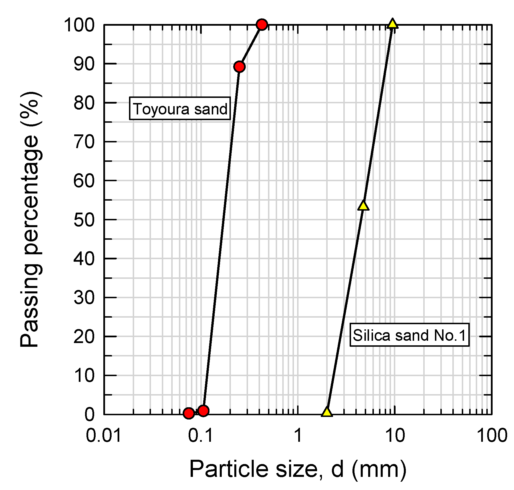
3.1. Soil Samples

The soil samples used for the CB model tests were represented by Toyoura sand (a standard sand in Japan) and silica sand No. 1 (as gravel material): Figure 2 shows their respective grain size distribution curves. The two soil samples had particle densities (ρ_s) of 2.64 and 2.65 g/cm³, mean particle sizes (D₅₀) of 1.69 and 4.65 cm, maximum dry densities (ρ_{d max}) of 1.64 and 1.67 g/cm³, minimum dry densities (ρ_{d min}) of 1.37 and 1.45 g/cm³, uniformity coefficients (C_u) of 1.63 and 2.24, and curvature coefficients (C_c) of 0.97 and 0.84, respectively. In the CB model tests described in Section 4, the relative density (D_r) of Toyoura sand (used for the sand layer) (ρ_d = 1.50 g/cm³) was 53.8%, while the relative density of silica sand No. 1 (used for the gravel layer) (ρ_d = 1.64 g/cm³) was 53.8%. Under the same conditions as the dry densities of Toyoura sand and silica sand No. 1, the saturated hydraulic conductivities (k_sat) of the two soil samples based on ASTM D2434-68 [45] were obtained as 1.45 × 10⁻⁴ m/s and 2.44 × 10⁻³ m/s, respectively. The physical properties and hydraulic conductivities of two soil samples are listed in

Table 1. Physical properties and hydraulic conductivities of the soil samples.

Sample	Toyoura Sand	Silica Sand No. 1
Soil particle density, ρs (g/cm3)	2.64	2.65
Mean particle size, D50 (cm)	1.69	4.65
Maximum dry density, ρd max (g/cm3)	1.64	1.67
Minimum dry density, ρd min (g/cm3)	1.37	1.45
Uniformity coefficient, Cu	1.63	2.24
Curvature coefficient, Cc	0.97	0.84
Relative density, Dr (%) in the CB model test	53.8	87.9
Saturated hydraulic conductivity, ksat (m/s)	1.45 × 10−4	2.44 × 10−3

.

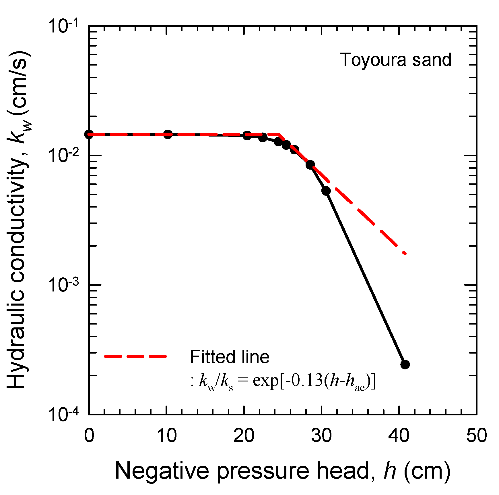
3.2. Water Retention Characteristics

The water retention characteristics of soils can be understood based on their respective SWCCs, representing the relationship between soil water and matric suction. In order to obtain the SWCCs of Toyoura sand and silica sand No. 1, we performed water retention tests through the continuous pressurization method [46]. Cylindrical specimens of 50 mm in diameter and 50 mm in height, with dry densities of 1.50 g/cm³ and 1.64 g/cm³, were used for these tests. The correspondent results were fitted by Equation (3) [34]. Figure 3a shows the fitted SWCCs resulting from the drying path of Toyoura sand and the wetting path of silica sand No. 1, related to the CB system. Specifically, in the CB system, since water infiltrates from the sand layer to the gravel layer below, the water retention characteristics of the sand and gravel layers correspond to the drying path where water is drained and the wetting path where water permeates, respectively. The fitting parameters of the SWCCs are summarized in

Table 2. Fitting parameters for the SWCCs.

Soil Sample	θs	AEV	EX	a	n	m
Toyoura sand	0.432	2.45	-	2.80	10.02	0.75
Silica sand No. 1	0.389	-	0.05	0.39	0.015	0.07

Note: AEV is the air entry value (kPa), EX is the air expulsion value, and θ_s is the saturated volumetric water content.

. An AEV of 2.30 kPa and an air expulsion value of 0.05 kPa were derived for Toyoura sand and silica sand No. 1, respectively. By comparing the SWCCs of the two soils, it was observed that there is a difference in the suction value for the volumetric water content between Toyoura sand and silica sand No. 1. As previously mentioned for the CB system, these different suction values indicate that the soils have distinct water retention capacities (of the water that infiltrates the sand layer) [12,16,41,47].

$$\theta =C(\psi ){\left\{\frac{{\theta }_s}{\ln [e+{(\psi /a)}^n]}\right\}}^m$$

(3)

where ψ is the total soil suction, e is the natural logarithmic constant (2.71828), a is a soil parameter related to the AEV of the soil (kPa), n a soil parameter that controls the slope at the inflection point along the soil–water retention curve, m a soil parameter related to the residual water content of the soil, and C(ψ) is the correction function that forces the soil–water retention curve through a suction of 1,000,000 kPa and zero water content. The correction function is given as follows:

$$\mathrm{C}(\psi )=\left[1-\frac{\ln (1+{\psi /\psi }_{\mathrm{r}})}{\ln (1+{10}^6{/\psi }_{\mathrm{r}})}\right]$$

(4)

where ψ_r is the suction value corresponding to the residual water content.

Since the water-shielding performance of the CB system is affected by the difference in hydraulic conductivity functions and soil-water characteristic curves between sand and gravel, it is very important to grasp the hydraulic conductivities (k_w) of the two samples. The relative hydraulic conductivities (k_r) of the Toyoura sand and silica sand No. 1 under the unsaturated condition in this study were estimated based on Equation (5) proposed by Fredlund et al. [48]. Here, Equation (5) for the relative hydraulic conductivity function was proposed by the combining Equation (3) with the statistical pore size distribution model of Childs and Collis-George [49]. Thus, the unsaturated hydraulic conductivities (k_w) of two samples were derived from the relationship between the saturated hydraulic conductivity (k_sat) and the relative hydraulic conductivity function (k_r). Figure 3b shows the results of the hydraulic conductivities of Toyoura sand and silica No. 1. It was found that the hydraulic conductivity of Toyoura sand is larger for the suction value of about 0.07 kPa or more, which is the intersection of the two results. This difference can also be understood in relation to the CB system’s capability of retaining infiltrated water.

$$k_r={\Theta }^q(\psi )\frac{{\displaystyle {\int }_{\ln (\psi )}^b\frac{\theta (e^y)-\theta (\psi )}{e^y}}{\theta }^{\prime }(e^y)dy}{{\displaystyle {\int }_{\ln ({\psi }_{aev})}^b\frac{\theta (e^y)-{\theta }_s}{e^y}}{\theta }^{\prime }(e^y)dy}$$

(5)

$$k_w=k_r\cdot k_{sat}$$

(6)

where k_r is the relative hydraulic conductivity, k_sat is the saturated hydraulic conductivity, Θ^q(ψ) is a correction factor (1.0), b is a constant of ln(10⁶), θ′ is the derivative of Equation (4), y is a dummy variable of integration representing suction, ψ_aev is the AEV of the soil, and θ_s is the saturated volumetric water content.

4. Laboratory SSCB Model Test under the Lateral No-Flow Condition

In this section, we describe a series of laboratory SSCB model tests, in which Toyoura sand and silica sand No. 1 were subjected to multiple rainfall intensities. In previous studies, large-scale CB model tests were carried out under the lateral no-flow condition. However, to efficiently evaluate the fluid diversion capacity of the CB system while reducing the test time and the cost of the SSCB model test, we investigated the infiltration behavior and the diversion length through an SSCB model test under the lateral no-flow condition. The diversion lengths obtained in this study were then compared with those estimated by an empirical equation under the lateral flow condition.

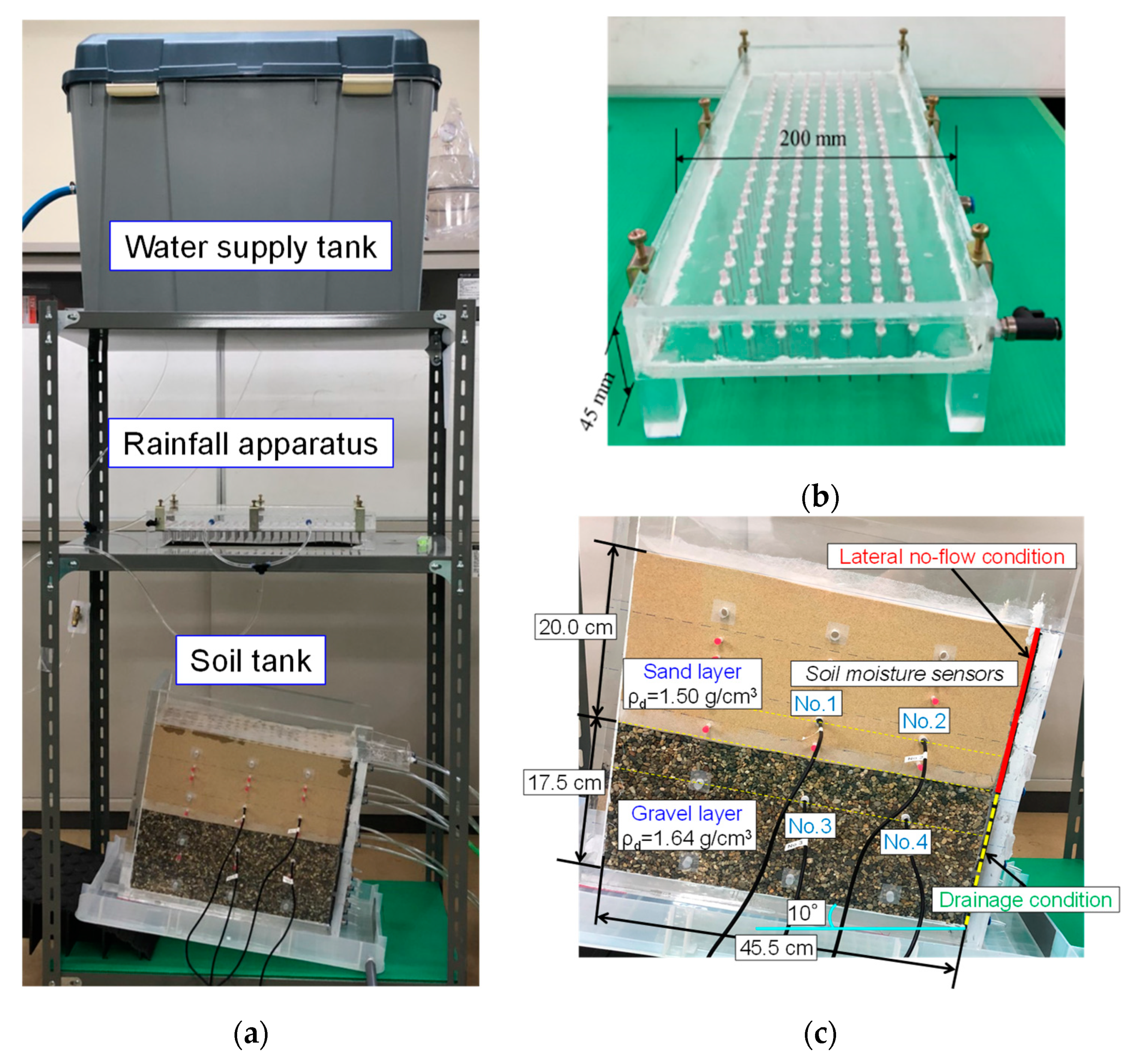
4.1. Apparatus and Conditions of the SSCB Model Test

The apparatus used for the CB model test included a water supply tank, a rainfall apparatus, and a soil tank (Figure 4a). The inside of the soil tank was 45.5 cm long, 47.0 cm high, and 15.0 cm wide; moreover, the thickness of the acrylic material was 20 mm. Figure 4b shows the rainfall apparatus, which was 500 mm long, 45 mm high, and 200 mm wide; furthermore, the thickness of the acrylic material was 5 mm. To properly reproduce the rainfall phenomenon, 161 needles were installed at 20 mm intervals (7 needles per row, over a total of 24 rows) in the lower part of the rainfall device. The sand and gravel layers were 20.0 cm and 17.5 cm high, respectively (Figure 4c); moreover, their initial dry densities (ρ_di) were 1.50 g/cm³ and 1.64 g/cm³, respectively. Differently from past studies conducted under the lateral flow condition, we installed some material (i.e., tarpaulin) to prevent drainage on the right side of the flow direction in the sand layer (Figure 4c). To ensure the drainage of water that infiltrated from the sand layer to the gravel layer, the right side of the gravel layer was set as a drainage condition. Thus, the experimental condition in the SSCB model test reproduces the extreme condition under which breakthrough forcibly occurs in the CB system as shown in Figure 1a, and which derives from the infiltration of rainfall from the sand layer. In other words, through the proposed SSCB model test, we expected to be able to quickly examine the performance of the CB system based on differences in water retention between the sand and gravel layers under certain experimental conditions. The diversion length measured in the SSCB model test is limited to the length of the soil tank, and the diversion length considered for the real CB system based on the results of the SSCB model test is discussed in detail in a later chapter.

Four holes were created in the apparatus of the SSCB model test for installing the soil moisture sensor, allowing the measurement of the volumetric water content 50 mm above and below the interface between the sand and gravel layers. Moreover, the water level in the water supply tank was kept constant, and the water used to reproduce different rainfall intensity (I) conditions was supplied by controlling a valve located between the rainfall apparatus and the water tank. The rainfall intensity conditions were the following: 20 mm/h (Case 1), 50 mm/h (Case 2), and 100 mm/h (Case 3). Notably, the slope angle of the soil tank was 10°. Four soil moisture sensors (EC-5, Decagon Devices Co.) were installed inside the soil tank to measure the variations in volumetric water content due to water infiltration. These sensors were able to measure soil moisture (i.e., volumetric water content) levels between 0 and 100%, and their precision was ±3.0% in the case of sandy soil. The performance of the CB system was hence evaluated by setting the duration of rainfall to 6 h under extreme conditions. Although the rainfall for 6 h in this study was applied as an extreme condition for evaluating the water-shielding performance of the CB system, further studies on the CB system applying rainfall patterns in specific regions would also be needed. After 6 h of rainfall with intensity I = 20 mm/h, the amount of drainage water was expected to reach a sufficiently steady condition, which was confirmed through a preliminary model test. The conditions of the laboratory SSCB model test under the lateral no-flow condition are summarized in

Table 3. Conditions of the SSCB model test.

Case No.		Case 1	Case 2	Case 3
Sand layer	Initial dry density, ρdi (g/cm3)	1.50	1.50	1.50
	Initial water content, wi (%)	0.64	1.11	0.33
	Initial volumetric water content, θi	0.01	0.02	0.01
Gravel layer	Initial dry density, ρdi (g/cm3)	1.64	1.64	1.64
	Initial water content, wi (%)	0.87	1.19	1.30
	Initial volumetric water content, θi	0.01	0.02	0.02
Drainage material: nonwoven fabric	Material (Fiber cross-section: ◎)	-Outside: polyethylene -Inside: polyester
	Thickness (mm)	0.13
	Hydraulic conductivity for vertical plane (m/s)	1.30 × 10−3
Rainfall intensity, I (mm/h)		20	50	100
Slope angle, Φ (°)		10	10	10
Measurement time (h)		6	6	6

.

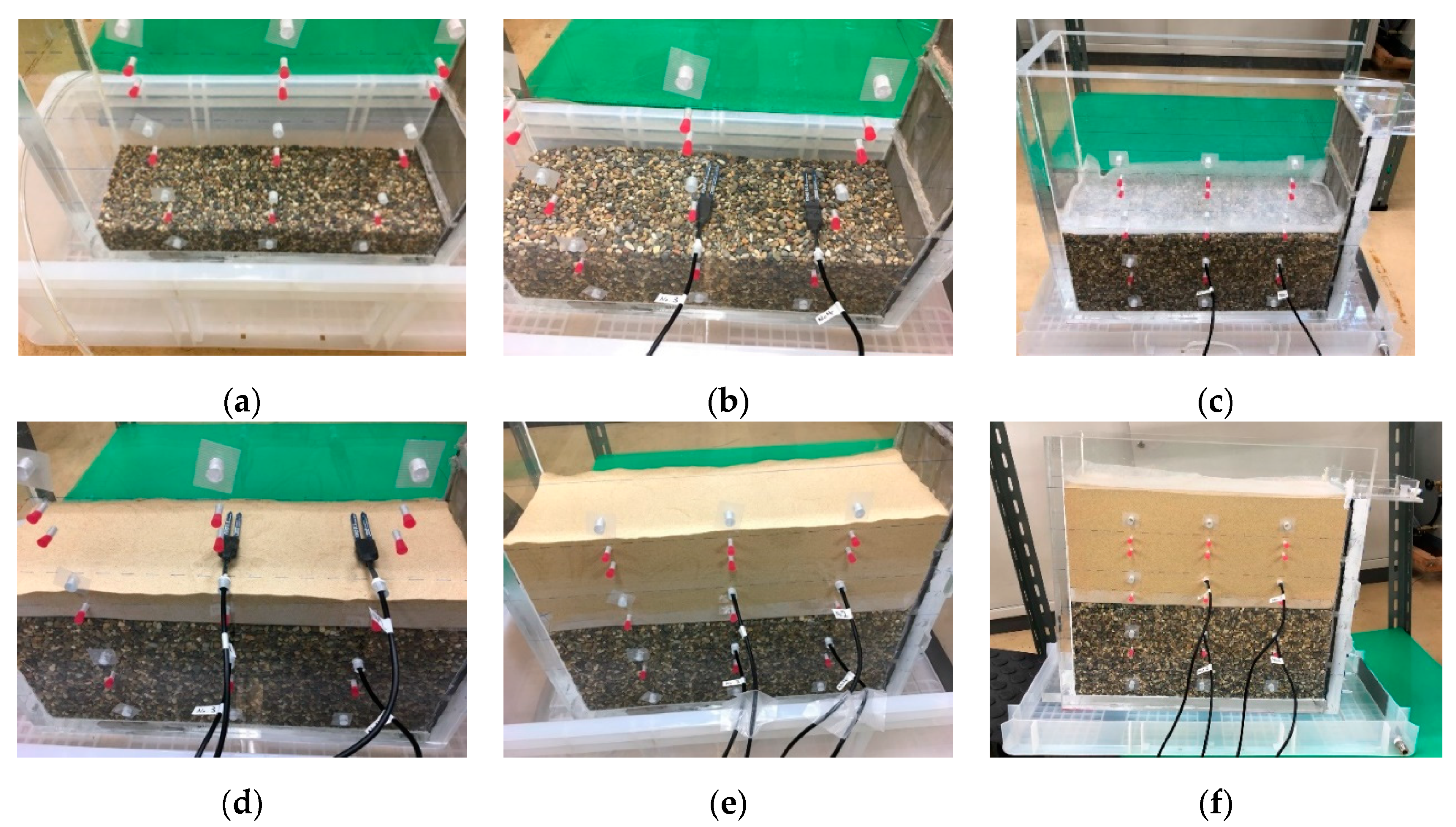
4.2. Production of the SSCB Model

The production process of the laboratory SSCB model is described below.

(1) The gravel layer composed of silica sand No. 1 was prepared in three steps. The first gravel layer, at the bottom of the soil tank, was prepared by maintaining a dry density of ρ_d = 1.64 g/cm³. Based on the baselines dividing it into 3 equal parts on the acrylic surface of the soil tank, the first gravel layer was prepared by the compaction method. (Figure 5a). (2) After the second gravel layer was prepared, the EC-5 sensors No. 3 and No. 4 were installed on its upper surface (Figure 5b). (3) After the third gravel layer was prepared, a drainage material with high water permeability was installed on its upper surface. Since the sand is smaller than the gravel, this drainage material prevents the sand (under dry conditions) from entering the gravel layer below (Figure 5c). The study by Kobayashi et al. [50] was reported that the diversion lengths obtained from the CB model tests were the same as each other regardless of the installation of drainage material (i.e., nonwoven fabric). The same drainage material was used in this study, and its specification is shown in Table 3. Thus, it can be said that the drainage material does not affect the water-shielding performance of the CB system in the SSCB model test. (4) The sand layer composed of Toyoura sand was prepared in three steps, similarly to the gravel layer, by maintaining a dry density of ρ_d = 1.64 g/cm³; then, the EC-5 sensors No. 1 and No. 2 were installed on the upper surface of the first sand layer (Figure 5d). (5) The drainage material was installed on the upper surface of the sand layer to prevent its erosion by rainfall during the SSCB model test. This drainage material was the same as the one installed at the interface between the gravel and sand layers (Figure 5f). It should be noted that the installation of the drainage material on the surface of the gravel layer is only a temporary measure to prevent the erosion by rainfall during the CB model test, and the drainage material is not installed on the surface of the real CB slope.

4.3. Preparation for the SSCB Model Test

First, the water tank was filled with water to a certain level; subsequently, as the water level lowered, new water was automatically supplied by the water level maintenance system. Regarding the rainfall apparatus, it was filled with water to ensure constant rainfall production and the constant filling of the tube connecting it to the water tank. Water fell from the rainfall system due to its own pressure, which derived from the height difference between the water tank and the rainfall apparatus. The rainfall intensity was adjusted by using a valve installed between the tubes. Before the experiment, we determined the conditions of the valve suitable for rainfall intensities of 20, 50, and 100 mm/h. As explained in Figure 4b, since the rainfall was reproduced by needles installed at intervals of 2.0 cm, it was applied to uniformly permeate rainfall over an average area of 4.0 cm². To consider only the effect of the rainfall infiltration on the ground surface in the SSCB model test, since the kinetic energy by water droplets from the rainfall apparatus to the surface of a sandy layer was neglected because it was very small. Then, the soil tank containing the sand and gravel layers was inclined to an angle of 10° to ensure the falling of rainfall on the sand layer. The variations in soil moisture were measured every 5 min for 6 h (the duration of the model test); furthermore, during the model test, the amount of water expelled from the soil tank was measured every hour and adjusted to keep each tested rainfall intensity constant over the experimental period.

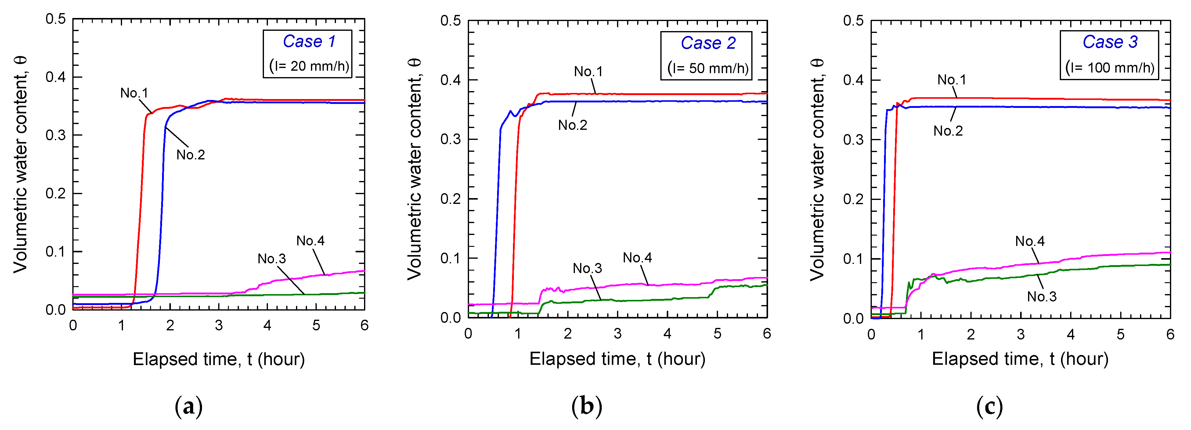
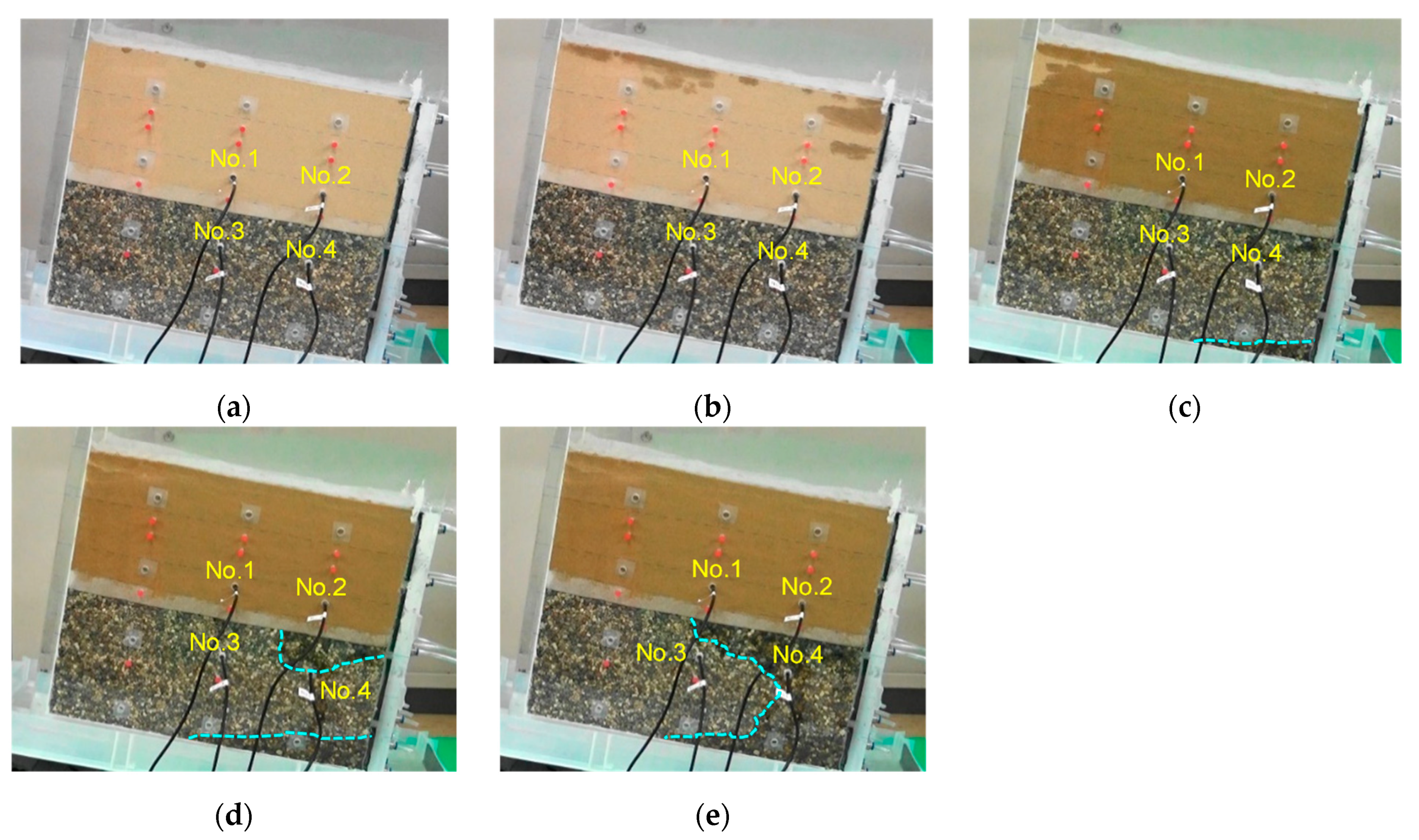
4.4. Infiltration Behavior in the SSCB Model Test

4.4.1. Result for Case 1

Figure 6 shows the results of the volumetric water contents (θ) measured by the EC-5 sensors for each case. It was observed that the measured values of sensors No. 3 and No. 4 after the breakthrough commonly increased up to 6 h. This tendency corresponds to a change according to the contact area with the sensor in the water infiltration paths. Thus, the infiltration path after 6 h in this study was also investigated, and the occurrence of an additional water infiltration path was not confirmed. After 6 h, since the amount of water drained from the soil tank was in a steady state compared to the precipitation, we decided to conclude the model test. It should be also noted that there was no surface runoff or predominant lateral runoff for each case in this study.

The model test for Case 1 was performed under a rainfall intensity of 20 mm/h over 6 h (Table 3). Figure 6a shows the volumetric water contents (θ) measured by the EC-5 sensors for the model test of Case 1: the response times of the four EC-5 sensors were visibly different. In fact, at t = 75 min, sensor No. 1 (installed in the sand layer) showed the fastest response, indicating a rapid increase in the volumetric water content. Meanwhile, sensor No. 2 reported a rapid increase in the volumetric water content 10 min later than sensor No. 1; after which the volumetric water content appeared to quickly reach the saturated condition (as in the case of sensor No. 1). These results indicate that, in Case 1, the sand layer became saturated after 180 min. Notably, sensor No. 3 (installed in the gravel layer) did not show any response during the test. Finally, sensor No. 4 showed a gradual increase in the volumetric water content after 210 min, demonstrating the occurrence of a breakthrough at that time.

Figure 7 shows the occurrence of rainfall infiltration in Case 1 as a function of time. The infiltration of rainfall to the midpoint of the sand layer was observed after 60 min from the beginning of the test (dry state) (Figure 7a,b). After 200 min, the entire sand layer became saturated (Figure 7c). This trend was observed in terms of variations in the volumetric water content by sensors No. 1 and No. 2 (Figure 6a). Meanwhile, a breakthrough was clearly observed in Case 1 after 210 min (Figure 7d). After 360 min (6 h), sensor No. 4 indicated an increase in the volumetric water content due to rainfall infiltration; however, sensor No. 3 did not measure any increase, since it was located at a distance from the location of the breakthrough event (Figure 7e). Notably, after t = 360 min, the observations of all sensors agreed well with each other (Figure 6a).

4.4.2. Result for Case 2

The model test for Case 2 was performed under a rainfall intensity of 50 mm/h over 6 h (Table 3). As in Case 1, the amount of water that drained from the soil tank after 6 h was found in a steady state; hence, we concluded the model test at that time. Figure 6b shows the volumetric water contents (θ) measured by the EC-5 sensors for the model test of Case 2. Notably, the response times of sensors No. 1 and No. 2 in the sand layer under I = 20 mm/h were different from those measured in Case 1 (Figure 6b). In particular, sensor No. 1 started to respond 50 min after the start of the test and indicated a rapid increase in the volumetric water content within a short time after that. Meanwhile, sensor No. 2 started to respond 20 min earlier than sensor No. 1 (30 min after the start of the test), indicating a rapid increase in the volumetric water content until 60 min, when the saturation state was reached. The reason why sensor No. 1 reacted before sensor No. 2 in Case 1 could be that lower rainfall intensity (I) causes a predominantly vertical infiltration, and thus the increase in the volumetric water content was first detected by sensor No. 1. However, in Case 2 with higher rainfall intensity (I) at the upper boundary, it can be understood that the lateral no-flow boundary condition could cause the accumulation of water in the right corner of the model, and thus the increase in the volumetric water content was first detected at sensor No. 2 location. Since the results of both of these sensors showed high volumetric water contents at 85 min, we infer that the saturation of the sand layer in Case 2 was completed after that time. Moreover, sensors No. 3 and No. 4 in the gravel layer showed an increase in the volumetric water content at 85 min: a breakthrough should have occurred in Case 2 at that time. In Case 2, under a rainfall intensity of 20 mm/h, the saturation of the sand layer and the breakthrough occurred 95 min and 125 min, respectively, before those in Case 3.

4.4.3. Result for Case 3

The model test for Case 3 was performed under a rainfall intensity of 100 mm over 6 h (Table 3). As in Case 1 and Case 2, the amount of water that drained from the soil tank was found to be in a steady state after 6 h; hence, we decided to conclude the model test at that time. Figure 6c shows the volumetric water contents (θ) measured by the EC-5 sensors for the model test of Case 3: notably, the response times of sensors No. 1 and No. 2 in the sand layer were shorter in Case 3 than in Case 1 and Case 2 (Figure 6c). In fact, sensor No. 1 (installed in the sand layer) responded after 20 min, indicating a constant, high volumetric water content after 45 min. Sensor No. 2 responded 10 min earlier than sensor No. 1; in addition, in this case, a constant volumetric water content was measured after 45 min. Thus, we infer that the saturation of the sand layer in Case 3 was completed after 45 min. Meanwhile, sensors No. 3 and No. 4 in the gravel layer both showed an increase in the volumetric water content at 45 min, suggesting the occurrence of breakthrough at that time. The saturation and breakthrough of the sand layer in Case 3 occurred 160 and 165 min prior to those Case 1, respectively. Moreover, compared to Case 2, the saturation of the sand layer and the breakthrough in the same layer in Case 3 occurred both 40 min earlier than in Case 2. Overall, the results of the SSCB model tests for Case 1, Case 2, and Case 3 under I = 20, 50, and 100 mm/h, suggest that the rainfall intensity was very closely related to the time needed for reaching the saturation of the sand layer, as well as to the time of breakthrough occurring in the CB system. As summarized in

Table 4. Measurement results for each case.

No.	I (mm/h)	Time to Reach the Saturation State of the Sand Layer	Time of Breakthrough Occurrence
Case 1	20	180 min	210 min
Case 2	50	85 min	85 min
Case 3	100	45 min	45 min

, the two series of time data just mentioned are proportionally related to the rainfall intensity.

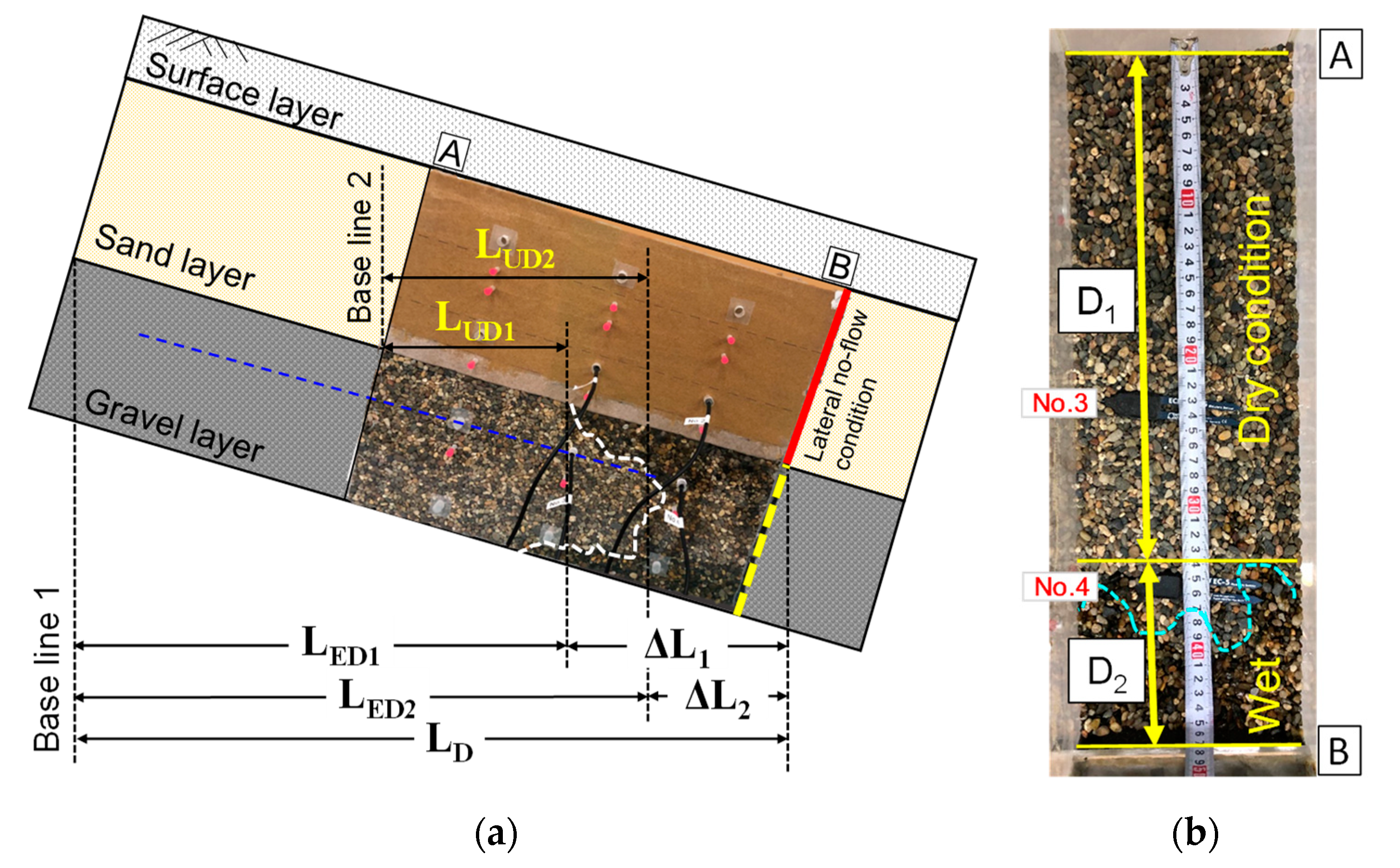
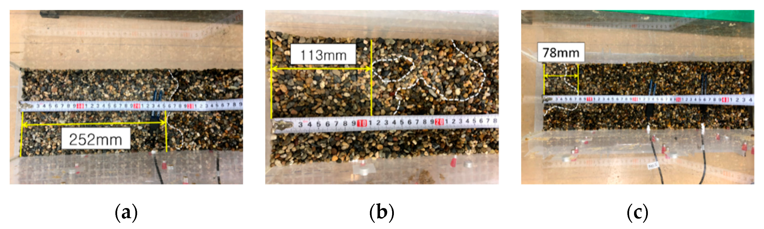
4.4.4. Measurement Results of the Diversion Lengths in the SSCB Model Test

Figure 8a shows a sample situation in which a breakthrough occurred under the lateral no-flow condition. Here, the area comprised between A and B corresponds to the size of the model used for the laboratory model test. The breakthrough point was not easy to identify, because water infiltration from the interface between the sand and the gravel layers did not occur regularly over time. In addition, to determine the pattern of rainfall infiltration according to the sensor responses, we defined two types of diversion lengths in the SSCB model test (Figure 8a). One of them is the distance, L_UD1 (i.e., the undrained diversion length), which was measured at the position of breakthrough occurrence from base-line 2 (at the interface between the sand and gravel layers). After the completion of the model test (at t = 360 min) (Figure 7e), the L_UD1 values for each case were determined based on the infiltration of water from the front and back sides of the model under steady conditions. The L_UD1 for Case 1, Case 2, and Case 3 were 13.5 cm, 11.7 cm, and 0 cm, respectively. Notably, the horizontal length of L_UD1 was calculated by considering the 10° slope angle. The other type of diversion length considered here was the distance from baseline 2 to the occurrence point of the finger flow (L_UD2) at the height of the soil moisture sensors (No. 3 and No. 4) installed in the gravel layer. After the completion of the model test, the sand and gravel layers were carefully dismantled up to the location of sensors installed in the gravel layer; then, the lengths of D₁ and D₂ were measured as shown in Figure 8b. Here, the lengths of D₁ and D₂ correspond to the dry and wet areas, respectively. The D₁ values obtained for Case 1, Case 2, and Case 3 were 25.2 cm, 11.3 cm, and 0 cm, respectively (Figure 9). Notably, although some dry areas were detected at 7.8 cm in Case 3 (Figure 9c), the correspondent D₁ value was determined as 0, since the left side of the soil tank was partially wet. The L_UD2 values were calculated using the following formula: L_UD2 = D₁·cosΦ, where Φ is the slope angle and those for Case 1, Case 2, and Case 3 were 24.8 cm, 11.2 cm, and 0 cm, respectively. The L_UD1 and L_UD2 values are all shown in

Table 5. Measured and estimated values of diversion length, L_D.

Case No.		Case 1	Case 2	Case 3
Rainfall intensity, I (mm/h)		20	50	100
Lateral nonflow condition	Measured LUD1 (cm)	13.5	11.7	0
	Measured LUD2 (cm)	24.8	11.2	0
Lateral flow condition	Estimated LD (cm) by Equation (2)	145.5	56.8	27.7
ΔL1 (cm)		31.3	33.1	44.8
ΔL2 (cm)		20.0	33.6	44.8
Effective diversion length, LED1 (cm)		114.2	23.7	−17.1
Effective diversion length, LED2 (cm)		125.5	23.1	−17.1

.

By comparing these results, we found that the larger the rainfall intensity, the larger the diversion length values were under the lateral no-flow condition. Notably, the highest diversion length values were found for Case 1, under I = 20 mm/h. In Case 2, under I = 50 mm/h, the L_UD1 and L_UD2 values were 13.3% and 54.8% lower than in Case 1. In Case 3, under extremely high rainfall intensity (I = 100 mm/h), our CB system collapsed. Since rainfall intensity has the greatest influence on the diversion lengths of the CB system, when designing such systems, it is fundamental to verify the maximum allowable value of rainfall intensity.

4.5. Diversion Length on the SSCB Model Test

The existing diversion length (L_D) under the lateral flow (drained) condition was derived, like in past studies, by using Equation (2) of Steenhuis et al. [28]. Each parameter related to Equation (2) was determined as follows. First, b was derived from the equation of the unsaturated hydraulic conductivity: the unsaturated permeability coefficient (k_w) of sand was approximated by applying the exponential function of the negative pressure head (h), as shown in Equations (7) and (8). In particular, since the seepage (i.e., the breakthrough) into the gravel layer from the sandy layer in the CB system occurs when the sand layer is close to saturation, the value of b for this condition in this study was applied. Thus, the value of b in this study was determined from the relationship of the instantaneous change in the permeability coefficient for increased suction from the AEV point. Based on the exponential approximation of the relationship between the unsaturated permeability coefficient and the negative pressure head for Toyoura sand (Figure 10), the value of b was estimated as 0.13.

$$k_w=k_{sat}h<h_{ae}$$

(7)

$$k_w=k_{sat}\exp [-b(h-h_{ae})]h>h_{ae}$$

(8)

Notably, the saturation permeability coefficient of Toyoura sand (k_sat) was 1.45 × 10⁻² cm/s, its slope angle (Φ) 10°, and its AEV (h_ae) 24.5 cm; moreover, the air expulsion value of silica sand No. 1 (h_aex) was 0.5 cm. For each case, we applied the following the κ values (= q_v/k_sat) and rainfall intensities: Case 1: q_v = 20 mm/h → κ = 0.038, Case 2: q_v = 50 mm/h → κ = 0.096, and Case 3: q_v = 100 mm/h → κ = 0.19. All the determined parameters (shown in

Table 6. Input parameters and results of the diversion length estimation done by applying Equation (2).

qv (mm/h)	ksat (cm/s)	κ	b	Φ (°)	hae (cm)	haex (cm)	LD (cm)
20	1.45 × 10−2	0.038	0.13	10	24.5	0.5	145.5
50		0.096					56.8
100		0.192					27.7

) were substituted into Equation (2) for each case, deriving the following diversion lengths (L_D) under the lateral flow (drained) condition: 145.5 cm (Case 1), 56.8 cm (Case 2), and 27.7 cm (Case 3). As such, the diversion length estimated by Equation (2) can be understood as the maximum theoretical water-shielding capability of the CB system. As explained earlier, it can be seen that the length of the diversion length is significantly affected by the rainfall intensity.

Meanwhile, the lengths of ΔL₁ and ΔL₂ were used to identify the wet areas of the gravel layer that formed due to breakthrough (Figure 8a). By considering ΔL₁ = L_st − L_UD1 and ΔL₂ = L_st − L_UD2, the following values were derived for ΔL₁ and ΔL₂: 31.3 and 20.0 cm (Case 1), 33.1 and 33.6 cm (Case 2), and 44.8 and 44.8 cm (Case 3), respectively. We indicated with L_st the horizontal length of the soil tank when considering the slope angle (i.e., L_st = 45.5 × cosΦ, in cm). The effective diversion lengths (L_ED1 and L_ED2) became smaller under the lateral no-flow condition: L_ED1 = L_D − ΔL₁ and L_ED2 = L_D − ΔL₂ (Figure 8a). L_ED1 represented the diversion length in the SSCB model test after it reached the level of the interface between the sand and gravel layers, while L_ED2 represented the diversion length in the CB model test after it reached the sensor installation level in the gravel layer. We obtained the following values for L_ED1 and L_ED2: 114.2 and 125.5 cm (Case 1), 23.7 and 23.1 cm (Case 2), and −17.1 and −17.1 cm (Case 1), respectively. Here, negative values of L_ED1 and L_ED2 (e.g., −17.1 and −17.1 cm for Case 3) indicated that the diversion length could not be formed under extreme rainfall (I = 100 mm/h), which means there is no water-shielding performance of the CB system. The results described above are summarized in Table 5.

Figure 11 compares the diversion lengths (L_D) estimated by Equation (2) and the L_ED1 and L_ED2 values obtained from the SSCB model test under the lateral no-flow condition in the sand layer. The resulting effective diversion lengths (i.e., L_ED1 and L_ED2) in the CB system were 21.5% and 13.8% lower in Case 1 and 58.3% and 59.2% lower in Case 2, respectively, than the L_D values estimated by Equation (2). In Case 3, under I = 100 mm/h, although the occurrence of a diversion length (L_D = 27.7 cm) was predicted by the empirical formula, no diversion length could be observed during the SSCB model test under the lateral no-flow condition. Our results indicate that the water-shielding performance of the CB system can be efficiently evaluated through the SSCB model test under the lateral no-flow condition, rather than through large-scale model tests. The size of the SSCB model can be appropriately adjusted based on the rainfall conditions or the soils used. It was concluded that the application of the results of the SSCB model test in the slope design of soil structures based on the CB system would be helpful for improving slope stability.

5. Summaries and Conclusions

In this study, the laboratory SSCB model tests were performed to efficiently evaluate the water-shielding performance of the CB system. Unlike in previous studies, our SSCB system was characterized by setting the drainage condition in the flow direction of the inclined sand layer as the lateral no-flow condition. Through the laboratory SSCB model tests, we tested three different rainfall intensities (i.e., 20, 50, 100 mm/h). To evaluate the effectiveness of the SSCB model test, the diversion lengths were estimated by the empirical equation for the lateral flow condition based on the physical and water retention characteristics of sand and gravel; then, these diversion lengths were compared to the results of the SSCB model test. The conclusions derived from the results of this study are summarized below.

• The inside of the SSCB model proposed in this study was 45.5 cm long, 47.0 cm high, and 15.0 cm wide. Notably, the amount of drainage water under the lowest tested rainfall intensity (I = 20 mm/h) reached a steady state within 6 h. We can hence infer that the production work and the testing results of the SSCB model were better when the testing time was relatively short. Moreover, since this model was smaller than the large-scale models described in previous works, it was expected that its production work and testing would have a lower cost.
• The following rainfall intensities were achieved during the SSCB model tests: 20 mm/h (Case 1), 50 mm/h (Case 2), and 100 mm/h (Case 3). The time required by the sand layer to reach the saturation state in each of the above cases was 180 min, 85 min, and 45 min, respectively; moreover, breakthroughs occurred at 210 min, 85 min, and 45 min, respectively. Thus, the rainfall intensity was very closely related both to the time required by the sand layer to reach the saturation state and to the time of breakthrough occurrence in the CB system.
• The diversion lengths in the SSCB model test of this study were measured based on two criteria (i.e., L_UD1: at the interface between the sand and the gravel layers, and L_UD2: the occurrence point of the finger flow at the height of the soil moisture sensors (No. 3 and No. 4) installed in the gravel layer), because water infiltration occurred irregularly from the interface between the sand and the gravel layers. The L_UD1 values obtained for Case 1, Case 2, and Case 3 were 13.5 cm, 11.7 cm, and 0 cm, respectively; meanwhile, the L_UD2 values were 24.8 cm, 11.2 cm, and 0 cm, respectively. These results indicate that L_UD1 and L_UD2 were 13.3% and 54.8% lower, respectively, in Case 2 (I = 50 mm/h) than those in Case 1 (I = 20 mm/h). Finally, in Case 3, under the extreme rainfall intensity of 100 mm/h, our CB system collapsed.
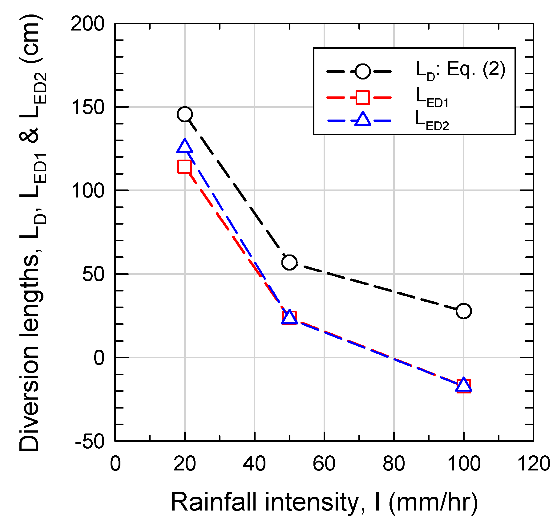
• The diversion lengths (L_D) under the lateral flow condition were estimated by the empirical equation of Steenhuis et al. [28] based on the hydraulic conductivity functions and soil-water characteristic curves of the sand and gravel. In Case 1, Case 2, and Case 3, they were 145.5 cm, 56.8 cm, and 27.7 cm, respectively. However, considering that the lengths of ΔL₁ and ΔL₂ would be reduced by the occurrence of breakthroughs in the SSCB model test, the effective diversion lengths (i.e., L_ED1 and L_ED2) for the real CB system were derived. The L_ED1 and L_ED2 values in Case 1, Case 2, and Case 3 were 114.2 and 125.5 cm, 23.7 and 23.1 cm, and −17.1 and −17.1 cm, respectively. Here, negative L_ED1 and L_ED2 values (i.e., −17.1 cm and −17.1 cm in Case 3) indicated that there is no water-shielding performance of the CB system under extreme rainfall (i.e., I = 100 mm/h).
• The diversion lengths in the CB system were compared: L_D (estimated by the empirical equation) and L_ED1 and L_ED2 (estimated based on the SSCB model test). The results indicated that L_ED1 and L_ED2 were lower than the correspondent L_D values, and that their reduction reflected the differences in rainfall intensity between one case and the other: the L_ED1 and L_ED2 values were 21.5% and 13.8% (Case 1), or 58.3% and 59.2% (Case 2) lower, respectively, than the correspondent L_D values. Thus, when the effective diversion lengths based on the SSCB model test are applied to the real CB system design, it is expected that since the reduced water-shielding performance of the CB system is taken into account, and the stability of the CB slope will be further improved. In addition, since the L_ED1 and L_ED2 values have a slight difference, applying the average of the two values to the CB system design may be a reasonable suggestion.

Based on the above results, we infer that the water-shielding performance of the CB system can be efficiently evaluated by conducting the proposed SSCB model tests under the lateral no-flow condition, rather than through large-scale model tests. Furthermore, the application of the results of the SSCB model test to the slope design of soil structures based on the CB system would be helpful for improving slope stability.

References

1. Miyazaki, T. Water flow in unsaturated soil in layered slopes. J. Hydrol. 1988, 102, 201–214. [Google Scholar] [CrossRef]
2. Rasmuson, A.; Eriksson, J.C. Capillary Barriers in Covers for Mine Waste Dumps; Report 3307; The National Swedish Environmental Protection Board: Stockholm, Sweden, 1986. [Google Scholar]
3. Nicholson, R.V.; Gillham, R.W.; Cherry, J.A.; Reardon, E.J. Reduction of acid generation in mine tailings through the use of moisture-retaining cover layers as oxygen barriers. Can. Geotech. J. 1989, 26, 1–8. [Google Scholar] [CrossRef]
4. Ross, B. The diversion capacity of capillary barriers. Water Resour. Res. 1990, 26, 2625–2629. [Google Scholar] [CrossRef]
5. Nyhan, J.W.; Schofield, T.G.; Starmer, R.H. A Water Balance Study of Four Landfill Cover Designs Varying in Slope for Semiarid Regions. J. Environ. Qual. 1997, 26, 1385–1392. [Google Scholar] [CrossRef]
6. Kämpf, M.; Montenegro, H. On the performance of capillary barriers as landfill cover. Hydrol. Earth Syst. Sci. 1997, 1, 925–930. [Google Scholar] [CrossRef] [Green Version]
7. Khire, M.V.; Benson, C.H.; Bosscher, P.J. Capillary barriers: Design variables and water balance. J. Geotech. Geoenviron. Eng. 2000, 126, 695–708. [Google Scholar] [CrossRef] [Green Version]
8. Bussière, B.; Aubertin, M.; Chapuis, R.P. The behavior of inclined covers used as oxygen barriers. Can. Geotech. J. 2003, 40, 512–535. [Google Scholar] [CrossRef]
9. Parent, S.É.; Cabral, A. Design of inclined covers with capillary barrier effect. Geotech. Geol. Eng. 2006, 24, 689–710. [Google Scholar] [CrossRef]
10. Corey, J.C.; Horton, J.H. Influence of Gravel Layers on Soil Moisture Content and Flow; Du Pont de Nemours (EI) and Co.: Aiken, SC, USA; Savannah River Lab.: Jackson, SC, USA, 1969. [Google Scholar] [CrossRef] [Green Version]
11. Hill, D.E.; Parlange, J.Y. Wetting front instability in layered soils. Soil Sci. Soc. Am. J. 1972, 36, 697–702. [Google Scholar] [CrossRef]
12. Morel-Seytoux, H.J. Dynamic perspective on the capillary barrier effect at the interface of an upper fine layer with a lower coarse layer. In Engineering Hydrology; ASCE: Reston, VA, USA, 1993; pp. 467–472. [Google Scholar]
13. Baker, R.S.; Hillel, D. Laboratory tests of a theory of fingering during infiltration into layered soils. Soil Sci. Soc. Am. J. 1990, 54, 20–30. [Google Scholar] [CrossRef]
14. Walter, M.T.; Kim, J.S.; Steenhuis, T.S.; Parlange, J.Y.; Heilig, A.; Braddock, R.D.; Selker, J.S.; Boll, J. Funneled flow mechanisms in a sloping layered soil: Laboratory investigation. Water Resour. Res. 2000, 36, 841–849. [Google Scholar] [CrossRef] [Green Version]
15. Tami, D.; Rahardjo, H.; Leong, E.C.; Fredlund, D.G. A physical model of sloping capillary barriers. Geotech. Test. J. 2004, 27, 11–27. [Google Scholar] [CrossRef] [Green Version]
16. Aubertin, M.; Cifuentes, E.; Apithy, S.A.; Bussière, B.; Molson, J.; Chapuis, R.P. Analyses of water diversion along inclined covers with capillary barrier effects. Can. Geotech. J. 2009, 46, 1146–1164. [Google Scholar] [CrossRef]
17. Rahardjo, H.; Santoso, V.A.; Leong, E.C.; Ng, Y.S.; Tam, C.P.H.; Satyanaga, A. Use of recycled crushed concrete and Secudrain in capillary barriers for slope stabilization. Can. Geotech. J. 2013, 50, 662–673. [Google Scholar] [CrossRef]
18. Tang, J.; Taro, U.; Huang, D.; Xie, J.; Tao, S. Physical Model Experiments on Water Infiltration and Failure Modes in Multi-Layered Slopes under Heavy Rainfall. Appl. Sci. 2020, 10, 3458. [Google Scholar] [CrossRef]
19. Boulanger-Martel, V.; Bussière, B.; Côté, J. Insulation covers with capillary barrier effects to control sulfide oxidation in the Arctic. Can. Geotech. J. 2021, 58, 583–594. [Google Scholar] [CrossRef]
20. Barth, C.; Wohnlich, S. Proof of effectiveness of a capillary barrier as surface sealing of sanitary landfill. In Proceedings of the 7th International Waste Management and Landfill Symposium, Santa Margarita di Pula, Cagliari, Italy, 4–8 October 1999; pp. 389–392. [Google Scholar]
21. Ng, C.W.; Liu, J.; Chen, R.; Xu, J. Physical and numerical modeling of an inclined three-layer (silt/gravelly sand/clay) capillary barrier cover system under extreme rainfall. Waste Manag. 2014, 38, 210–221. [Google Scholar] [CrossRef]
22. Zhan, T.L.; Li, H.; Jia, G.W.; Chen, Y.M.; Fredlund, D.G. Physical and numerical study of lateral diversion by three-layer inclined capillary barrier covers under humid climatic conditions. Can. Geotech. J. 2014, 51, 1438–1448. [Google Scholar] [CrossRef]
23. Matsumoto, K.; Kobayashi, K.; Morii, T.; Nakajusa, S. Evaluation of diversion length of the capillary barrier with nonflatness of regular sine wave shape between sand and gravel layers. Jpn. Geotech. J. 2016, 11, 305–313. (In Japanese) [Google Scholar] [CrossRef] [Green Version]
24. Park, T.W.; Kim, H.J.; Tanvir, M.T.; Lee, J.B.; Moon, S.G. Influence of coarse particles on the physical properties and quick undrained shear strength of fine-grained soils. Geomech. Eng. 2018, 14, 99–105. [Google Scholar] [CrossRef]
25. Oldenburg, C.M.; Pruess, K. On numerical modeling of capillary barriers. Water Resour. Res. 1993, 29, 1045–1056. [Google Scholar] [CrossRef]
26. Bussière, B.; Aubertin, M.; Chapuis, R.P. A laboratory set up to evaluate the hydraulic behavior of inclined capillary barriers. In Proceedings of the International Conference on Physical Modelling in Geotechnics, St. John’s, NL, Canada, 10–12 July 2002; pp. 391–396. [Google Scholar]
27. Morris, C.E.; Stormont, J.C. Evaluation of numerical simulations of capillary barrier field tests. Geotech. Geol. Eng. 1998, 16, 201–213. [Google Scholar] [CrossRef]
28. Steenhuis, T.S.; Parlange, J.-Y.; Kung, K.-S. Comment on “The diversion capacity of capillary barriers” by Benjamin Ross. Water Resour. Res. 1991, 27, 2155–2156. [Google Scholar] [CrossRef]
29. Bossi, G.; Borgatti, L.; Gottardi, G.; Marcato, G. The Boolean Stochastic Generation method-BoSG: A tool for the analysis of the error associated with the simplification of the stratigraphy in geotechnical models. Eng. Geol. 2016, 203, 99–106. [Google Scholar] [CrossRef]
30. Pasculli, A.; Calista, M.; Sciarra, N. Variability of local stress states resulting from the application of Monte Carlo and finite difference methods to the stability study of a selected slope. Eng. Geol. 2018, 245, 370–389. [Google Scholar] [CrossRef]
31. Sekhavatian, A.; Choobbasti, A.J. Comparison of Point Estimate and Monte Carlo probabilistic methods in stability analysis of a deep excavation. Int. J. Geo-Eng. 2018, 9, 1–19. [Google Scholar] [CrossRef]
32. Likos, W.J.; Lu, N. Hysteresis of capillary stress in unsaturated granular soil. J. Eng. Mech. 2004, 130, 646–655. [Google Scholar] [CrossRef]
33. Henry, E.J. Analytical and numerical modeling assessment of capillary barrier performance degradation due to contaminant-induced surface tension reduction. J. Geotech. Geoenviron. Eng. 2007, 133, 231–236. [Google Scholar] [CrossRef]
34. Fredlund, D.G.; Xing, A. Equations for the soil-water characteristic curve. Can. Geotech. J. 1994, 31, 521–532. [Google Scholar] [CrossRef]
35. Stormont, J.C. The effectiveness of two capillary barriers on a 10% slope. Geotech. Geol. Eng. 1996, 14, 243–267. [Google Scholar] [CrossRef]
36. Stormont, J.C.; Morris, C.E. Method to estimate water storage capacity of capillary barriers. J. Geotech. Geoenviron. Eng. 1998, 124, 297–302. [Google Scholar] [CrossRef] [Green Version]
37. Porro, I. Hydrologic behavior of two engineered barriers following extreme wetting. J. Environ. Qual. 2001, 30, 655–667. [Google Scholar] [CrossRef] [Green Version]
38. Abdolahzadeh, A.M.; Lacroix Vachon, B.; Cabral, A.R. Evaluation of the effectiveness of a cover with capillary barrier effect to control percolation into a waste disposal facility. Can. Geotech. J. 2011, 48, 996–1009. [Google Scholar] [CrossRef]
39. Kenney, T.; Chahal, R.; Chiu, E.; Ofoegbu, G.; Omange, G.; Ume, C. Controlling constriction sizes of granular filters. Can. Geotech. J. 1985, 22, 32–43. [Google Scholar] [CrossRef]
40. Dallo, Y.A.; Wang, Y. Determination of controlling constriction size from capillary tube model for internal stability assessment of granular soils. Soils Found. 2016, 56, 315–320. [Google Scholar] [CrossRef]
41. Morris, C.E.; Stormont, J.C. Parametric study of unsaturated drainage layers in a capillary barrier. J. Geotech. Geoenviron. Eng. 1999, 125, 1057–1065. [Google Scholar] [CrossRef] [Green Version]
42. Kung, K.-J.S. Preferential flow in a sandy vadose soil: 2. Mechanism and implications. Geoderma 1990, 46, 59–71. [Google Scholar] [CrossRef]
43. Kojima, M.; Miyazaki, T. Diversion capacity of capillary barriers on curved boundary slopes. Trans. JSIDRE 2004, 232, 395–402. (In Japanese) [Google Scholar] [CrossRef]
44. Morii, T.; Takeshita, Y.; Inoue, M.; Matsumoto, S. Field measurement of rainfall infiltration in capillary barrier of soil and determination of its divergence length. Trans. Jpn. Soc. Irrig. 2010, 77, 559–565. (In Japanese) [Google Scholar] [CrossRef]
45. ASTM D2434-68. Standard Test Method for Permeability of Granular Soils (Constant Head) (Withdrawn 2015); ASTM International: West Conshohocken, PA, USA, 2006. [CrossRef]
46. Kim, B.S.; Hatakeyama, M.; Park, S.W.; Park, H.S.; Takeshita, Y.; Kato, S. Assessment of water retention test by continuous pressurization method. Geotech. Test. J. 2021, 44, 274–289. [Google Scholar] [CrossRef]
47. Warrick, A.W.; Wierenga, P.J.; Pan, L. Downward water flow through sloping layers in the vadose zone: Analytical solutions for diversions. J. Hydrol. 1997, 192, 321–337. [Google Scholar] [CrossRef]
48. Fredlund, D.G.; Xing, A.; Huang, S. Predicting the permeability function for unsaturated soils using the soil-water characteristic curve. Can. Geotech. J. 1994, 31, 533–546. [Google Scholar] [CrossRef]
49. Childs, E.C.; Collis-George, N. The permeability of porous materials. Proc. R. Soc. Lond. Ser. A Math. Phys. Sci. 1950, 201, 392–405. [Google Scholar] [CrossRef] [Green Version]
50. Kobayashi, K.; Matsumoto, K.; Nakajusa, S.; Morii, T. Effect of the nonwoven fabric laying to give to diversion length of the capillary barrier. Jpn. Geotech. J. 2013, 8, 611–620. [Google Scholar] [CrossRef] [Green Version]
Figure 1. Concept of the CB system and capillary tube model: (a) concept of the CB system; (b) capillary tube model.
Applsci 11 05231 g001
Figure 2. Grain size distribution curves of Toyoura sand and silica sand No. 1.
Applsci 11 05231 g002
Figure 3. SWCCs and hydraulic conductivities of Toyoura sand and silica sand No. 1: (a) SWCCs; (b) hydraulic conductivities.
Applsci 11 05231 g003
Figure 4. Apparatus and conditions of the laboratory SSCB model test under the lateral no-flow condition: (a) apparatus of the SSCB model test; (b) rainfall apparatus; (c) setting conditions.
Applsci 11 05231 g004
Figure 5. Steps for the preparation of the laboratory SSCB model: (a) installation of the first gravel layer; (b) installation of sensors No. 3 and No. 4; (c) installation of the drainage material; (d) installation of the first sand layer and of sensors No. 1 and No. 2; (e) installation of the second sand layer; (f) after the sand layer was completed, the drainage material was laid on it.
Applsci 11 05231 g005
Figure 6. Measured volumetric water contents (θ) for each case: (a) Case 1 (I = 20 mm/h); (b) Case 2 (I = 50 mm/h); (c) Case 3 (I = 100 mm/h).
Applsci 11 05231 g006
Figure 7. Occurrence of rainfall infiltration as a function of the elapsed time in Case 1: (a) initial condition; (b) after 60 min; (c) after 200 min; (d) after 210 min; (e) after 360 min.
Applsci 11 05231 g007
Figure 8. Definition of each length in the SSCB model test under the lateral no-flow condition: (a) definition of the diversion lengths (LD, and LED1 and LED2); (b) definition of D1 and D2.
Applsci 11 05231 g008
Figure 9. Measurement results of D1 for each case: (a) Case 1; (b) Case 2; (c) Case 3.
Applsci 11 05231 g009
Figure 10. Exponential approximation of the relationship between the unsaturated permeability coefficient and the negative pressure head for Toyoura sand.
Applsci 11 05231 g010
Figure 11. Comparison of the diversion lengths based on the SSCB model test under the lateral no-flow condition and estimated by the empirical equation.
Applsci 11 05231 g011