Research on Extended Finite Element Method for Axisymmetric Electrostatic Field Based on Liquid Nitrogen with Bubbles

Abstract

In this paper, the extended finite element method (XFEM) is first applied to account for the weak discontinuity of the axisymmetric electrostatic field. Firstly, the interface between two materials in an element is described by the level set method. The enrichment function is used to modify the shape function of enrichment elements. Secondly, to illustrate the feature of the enrichment function, the distribution diagrams of enrichment functions in sub-elements are drawn. The 3D field can be simplified to an axisymmetric field, which can reduce the difficulty of calculation. Finally, models with bubbles in liquid nitrogen in the axisymmetric field are used to prove the reliability of XFEM. Compared with the conventional finite element method (CFEM), XFEM costs lower computing resources with almost the same computational accuracy.

1. Introduction

Insulation characteristics are one of the key factors that affect the reliability and safety of power equipment. The insulation problems of traditional power equipment and the more complex and diverse internal insulation problems in low-temperature environments need to be considered. The bubble problem in liquid nitrogen is one of internal insulation problems for high-temperature superconductivity equipment. Insulation design of high-temperature superconducting power equipment requires accurate knowledge of the electric potential distribution in the liquid nitrogen environment containing bubbles. Hence, an accurate and effective numerical calculation method is needed.

Many researchers have experimentally studied the dynamic characteristics of bubbles in the electric field [1,2,3,4] and found that bubbles have complex motion and deformation. However, few numerical methods are presented to analyze the electric potential.

The most common numerical method is the conventional finite element method (CFEM). However, CFEM requires a continuous interpolation function, and the material is not allowed to be changed in an element. Due to the small volume, large amount, and continuous motion of bubbles, it is difficult to calculate the electric potential characteristics of liquid nitrogen quickly and accurately with CFEM.

The extended finite element method (XFEM), an emerging numerical analysis method, has been developed to deal with extremely discontinuous problems based on CFEM. Compared with CFEM, it has significant advantages:

• The interfaces are described by the level set method. A special enrichment term is constructed to reflect the discontinuity characteristics. Therefore, XFEM can better solve the non-convergence problem caused by the discontinuity. For example, the sharp corner problem may lead to a non-converge in CFEM. However, XFEM can solve this problem well.
• The mesh reconstruction is effectively avoided when involving the moving boundary problems, because an element is allowed to contain two materials. XFEM can calculate each moment of bubble movement using only one set of mesh.

XFEM [5,6,7,8] developed from solid mechanics. XFEM has become the most popular computational tool in analyzing crack problems [9]. Muixí et al. [10] presented a combined XFEM phase-field model with sharp and diffuse representations of cracks, which divides the phase field and XFEM into two regions to simplify the calculation. The XFEM method has also been used by many scholars to solve the crack problem of piezoelectric materials. Gulab Pamnani et al. [11] used XFEM to analyze static impermeable cracks at the interface of piezoelectric materials. Mishra, R. et al. [12] predicted fatigue-cracking behavior of piezo-electric structures in the existence of multiple geometrical discontinuities under cyclic thermal-electrical-mechanical loads using XFEM. Zhang, C. et al. [13] used XFEM to solve the inverse problem of detecting multiple cracks in two-dimensional piezoelectric structures under dynamic electric loads. In the field of electrical engineering, Duan et al. [14] introduced the XFEM into the electric field analysis first. Wang [15] used the XFEM to calculate the electric field of an insulating plate with cracks. Duan et al. [16] proposed an improved XFEM for modeling electromagnetic devices with multiple nearby and applied it to the iron core. XFEM is used to analyze a field-circuit coupled high-temperature superconducting cable considering magnetic hysteresis [17]. As for the use of XFEM in an axisymmetric electric field, it is blank before.

In this paper, XFEM is first applied to analyze the discontinuity problems in an axisymmetric electric field. It could be used to analyze the electric field characteristics of transformer oil with bubbles, to calculate the current distribution in the conductive layer of high-temperature superconducting cable. Additionally, it also could be used for the calculation of magnetic field and eddy current distribution in the dense thin layer of transformer core and other practical situations.

2. Principle of Axisymmetric Extended Finite Element Method

The essence of XFEM is to use the enrichment function to modify the shape function of CFEM to achieve the purpose of describing discontinuities. The convergence of XFEM is ensured by the partition of unity method (PUM) [18]. The enrichment function is constructed by the level set function and the shape function of CFEM [19].

The axisymmetric field problems are studied on the (ρ, z) plane in the cylindrical coordinate system. The axisymmetric field can simplify 3D problems effectively, as shown in Figure 1. It has obvious advantages in improving computational efficiency with accuracy.

Figure 2 represents a sphere located in the middle of a cylinder. The elements containing the interface are called the enrichment elements as E. The nodes related to the enrichment elements are named enrichment nodes.

XFEM is a method that equates the boundary value problems of partial differential equations to the conditional variational problem. It establishes corresponding discrete equations to solve them. By dividing the solution domain into discrete finite elements, computations are made based on the node of these elements. The Poison boundary value problem of the axisymmetric electrostatic field is used in this paper.

$$\{\begin{array}{l}\mathsf{\Omega }:-\frac{1}{\rho }\frac{\partial }{\partial \rho }(\epsilon \rho \frac{\partial \phi }{\partial \rho })-\frac{\partial }{\partial z}(\epsilon \frac{\partial \phi }{\partial z})=\sigma \\ {\mathsf{\Gamma }}_1:\phi (\rho ,z)={\phi }_0\\ {\mathsf{\Gamma }}_1:\frac{\partial \phi (\rho ,z)}{\partial n}=0\end{array},$$

(1)

where $\mathsf{\Omega }$ is the solution domain, ${\mathsf{\Gamma }}_1,{\mathsf{\Gamma }}_1$ is the boundary, φ is the value of electric potential, ρ and z are the vertical coordinates of cylindrical coordinates, $\epsilon$ is the relative permittivity of a medium, $\sigma$ is surface charge density, ${\phi }_0$ is the electric potential at the boundary.

The approximation of the electric potential φ(ρ, z) (axisymmetric model) with triangular element mesh can be written as:

$$\phi (\rho ,z)={\displaystyle \sum _{i=1}^3{N}_i(\rho ,z){\phi }_i}+{\displaystyle \sum _{j=1}^m{N}_j(\rho ,z)\Phi (\rho ,z){\beta }_j},$$

(2)

where $N_i$, $N_j$ are the shape functions of CFEM, $\Phi$ is the enrichment function (its expression is as the Equation (3)), m is the number of the enrichment nodes in the enrichment element, ${\phi }_i$ and ${\beta }_j$ are unknowns.

$$\Phi (\rho ,z)={\displaystyle \sum _I{N}_I(\rho ,z)\cdot \left|{\varphi }_I\right|}-\left|{\displaystyle \sum _I{N}_I(\rho ,z)}\cdot {\varphi }_I\right|,$$

(3)

where ${\varphi }_I$ is the level set function.

The final equilibrium equation can be expressed in a discrete form as follows:

$$\left[\begin{array}{cc}{K}_{II}& K_{IJ}\\ K_{JI}& K_{JJ}\end{array}\right]\left\{\begin{array}{c}{\mathit{\phi }}_I\\ {\mathit{\phi }}_J\end{array}\right\}=\left\{\begin{array}{c}{P}_I\\ P_J\end{array}\right\},$$

(4)

where $K_{II}$,$K_{JJ}$ are the self-stiffness matrixes of FEM and enrichment nodes, respectively; $K_{IJ}$,$K_{JI}$ are the mutual stiffness matrixes between the two types of nodes.

The stiffness matrix is calculated by a minimum of energy functional of the axisymmetric field as:

$$\begin{array}{l}\frac{\partial W(\phi )}{\partial {\phi }_i}=\frac{2\pi \epsilon ({\rho }_i+{\rho }_j+{\rho }_m)}{3}{\displaystyle \underset{D}{\iint }(\frac{\partial {\phi }^e}{\partial \rho }\cdot \frac{\partial (\partial {\phi }^e/\partial \rho )}{\partial {\phi }_i}+\frac{\partial {\phi }^e}{\partial z}\cdot \frac{\partial (\partial {\phi }^e/\partial z)}{\partial {\phi }_i})d\rho dz}\\ \frac{\partial W(\phi )}{\partial {\beta }_i}=\frac{2\pi \epsilon ({\rho }_i+{\rho }_j+{\rho }_m)}{3}{\displaystyle \underset{D}{\iint }(\frac{\partial {\phi }^e}{\partial \rho }\cdot \frac{\partial (\partial {\phi }^e/\partial \rho )}{\partial {\beta }_i}+\frac{\partial {\phi }^e}{\partial z}\cdot \frac{\partial (\partial {\phi }^e/\partial z)}{\partial {\beta }_i})d\rho dz}\end{array},$$

(5)

where $W(\phi )$ is the energy functional. There is a coefficient in the formula that makes the axisymmetric field different from the parallel plane field.

3. Numerical Examples

Use enrichment function in Equation (3) and take the center of the circle as the origin of cylindrical coordinate. The boundary of the bubble in the field can be described using the level set function.

$$\varphi (\rho ,z)=\frac{{(\rho -{\rho }_0)}^2}{a^2}+\frac{{(z-z_0)}^2}{b^2}-R^2,$$

(6)

where (ρ, z) is the coordinate point in the cylindrical coordinate.

Three numerical models are used to verify the reliability of XFEM. Figure 3 shows an electric field analysis model of a bubble in the middle of cylindrical liquid nitrogen. The cylinder domain is simplified to an axisymmetric domain for more convenient calculation. The width of the axisymmetric domain is 7.5 mm and the height is 25 mm. The imposed voltage U is 8 V. The radii of bubbles are different in each model. The liquid nitrogen’s relative permittivity is 1.434, while the bubble’s is 1.

Mesh is important for the finite element method, and the quantity of elements is one of the key factors affecting the accuracy of the calculation. The more elements and nodes there are, the higher the accuracy of calculation there is. However, at the same time, it will consume more computing resources. Therefore, the appropriate mesh needs to be selected. Four meshes with different densities are selected in Figure 4. The electric potentials at all nodes are compared, and ten results are shown in

Table 1. Comparison of 10 nodal electric potentials of four kinds of meshes.

Point	Mesh-a	Mesh-b	Mesh-c	Mesh-d
(7.446, 4.482)	7.4356	7.4361	7.4362	7.4362
(5.817, −4.303)	4.6215	4.6212	4.6211	4.6211
(7.141, 4.514)	7.4456	7.4461	7.4462	7.4462
(2.405, −4.024)	4.7075	4.7073	4.7072	4.7072
(3.319, −1.273)	5.5895	5.5893	5.5890	5.5890
(1.553, 1.922)	6.6287	6.6295	6.6299	6.6301
(7.324, −9.541)	2.9463	2.9462	2.9461	2.9461
(3.412, 3.803)	7.2199	7.2205	7.2208	7.2208
(5.218, −3.169)	4.9840	4.9838	4.9837	4.9837
(6.383, 10.566)	9.3816	9.3817	9.3817	9.3817

.

The results of mesh-c and mesh-d at these nodes are basically the same. The solution can be confirmed as an exact one. The results of numerical solution change little as the number of elements increases. Therefore, mesh-d is the most appropriate choice. The selection of XFEM mesh is based on the CFEM. Additionally, the size of the element is the same at the position far away from bubbles, which ensures the mesh of the two calculation methods is of the same level.

3.1. Example 1

This example is solved by three methods, analytic method, CFEM, and XFEM. The electric potential in the bubble and the liquid nitrogen can be obtained by the method of separation of variables in spherical coordinates [20].

$$\begin{array}{l}{\phi }_{\mathrm{a}\mathrm{i}\mathrm{r}}=-\frac{3{\epsilon }_l}{{\epsilon }_a+2{\epsilon }_l}{E}_{0}rsin\theta +6\\ {\phi }_{\mathrm{l}\mathrm{i}\mathrm{q}\mathrm{u}\mathrm{i}\mathrm{d}}=-\left(1-\frac{{\epsilon }_a-{\epsilon }_l}{{\epsilon }_a+2{\epsilon }_l}\frac{R^3}{r^3}\right)E_{0}rsin\theta +6\end{array}$$

(7)

where ${\phi }_{\mathrm{a}\mathrm{i}\mathrm{r}}$ is the electric potential in the bubble, ${\phi }_{\mathrm{l}\mathrm{i}\mathrm{q}\mathrm{u}\mathrm{i}\mathrm{d}}$ is the electric potential in liquid nitrogen, $E_0=-\frac{U}{d}=-\frac{8}{25} \mathrm{V}/\mathrm{m}\mathrm{m}$ is the electric field intensity between two electrodes, R is the radius of the bubble. ${\epsilon }_l$, ${\epsilon }_a$ are the relative permittivity of liquid and bubble, r and $\theta$ can be converted to an axisymmetric coordinate system, which can be expressed as

$$r=\sqrt{{\rho }^2+z^2},\theta =\arctan \frac{z}{\rho },$$

(8)

Figure 5 shows the mesh of liquid nitrogen with a static bubble on XFEM and CFEM. The center of the circle is $(0,0)$. The radius of the bubble is 1.5 mm.

Based on the mesh in Figure 5, the enlarged diagram is shown in Figure 2. The element E contains two sub-elements (e and e₁). The enrichment function of the chosen element can be obtained as Figure 6 and Figure 7, which varies from different perspectives.

From the distribution diagrams of the enrichment function imposed on the element E, the characteristics of enrichment function can be summarized as follows:

• The values on nodes of enrichment elements and inside the conventional elements are zero.
• Meanwhile, the values inside the enrichment elements are positive.
• The maximum of the values is located on the interface.

Based on the above analysis, the electric potential of the axisymmetric field model is obtained by programming with XFEM. An enlarged view of the electric potential around the bubble is shown in Figure 8.

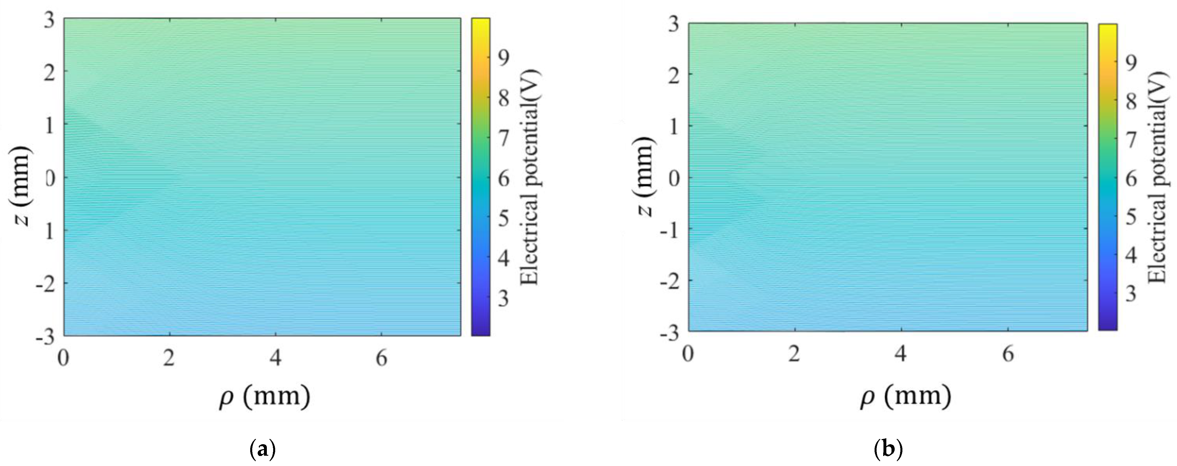
Comparing Figure 8a,b, the calculation results between XFEM and CFEM have little difference. The electric potentials of all XFEM nodes are selected for comparison. The relative errors of XFEM and analytic solutions, as well as the relative errors of XFEM and CFEM are shown in

Table 2. Relative error of electric potentials on nodes.

Method	Maximum Relative Error (%)	Average Relative Error (%)
XFEM-analytic method	0.15%	0.01%
XFEM-CFEM	0.22%	0.02%

.

The relative error is shown in Equation (9).

$$Relative Error=\frac{\phi -{\phi }_{\mathrm{X}\mathrm{F}\mathrm{E}\mathrm{M}}}{\phi }\times 100\%,$$

(9)

The error is related to the algebraic difference of point to point of two functions. $\phi$ is the electric potential of a point obtained by the analytic method or CFEM, and ${\phi }_{\mathrm{X}\mathrm{F}\mathrm{E}\mathrm{M}}$ is the electric potential of the same point obtained by XFEM. The maximum relative error is the largest error among all the nodes. The average relative error is the average of the norm of relative errors at all nodes.

The relative errors are small, which can verify the calculation results of XFEM are reliable.

3.2. Example 2

Figure 9 shows a model with four static bubbles in liquid nitrogen. The radii of these four bubbles from bottom to top are 1.3 mm, 1.5 mm, 1 mm, 1.7 mm. The electric potential results of bubbles in liquid nitrogen are obtained by XFEM and CFEM and shown in Figure 10.

In Figure 10, x and y represent the coordinate value of the node, and level represents the electric potential at the node. The difference of electric potential between CFEM and XFEM at the same node is very small. Statistically, the maximum relative error is 0.29%, and the average relative error is 0.03%.

3.3. Example 3

The behavior of bubbles in liquid nitrogen under the action of electric force includes two aspects: deformation and movement. The movement and deformation of the bubble under the electric field is determined by the electric force, surface tension, and gravity acting on the bubbles. Experiments show that bubbles are stretched into ellipsoids along the direction of the electric field intensity. The magnitude of the deformation is related to the intensity values.

With the deformation and movement of bubbles, remesh is required in CFEM. The complicated movement process of bubbles will significantly increase the calculation cost. XFEM can solve this problem by involving multiple media in one element.

Figure 11 shows the four steps of the process of movement and deformation of a bubble in the electric field with CFEM. In contrast, XFEM only meshed once as Figure 9b.

Figure 12 presents the electric potential of the moving bubble calculated with CFEM and XFEM.

The relative errors in each moment of electric potential based on CFEM and XFEM are shown in

Table 3. Electric potentials on nodes by using CFEM and XFEM.

Model	Maximum Relative Error (%)	Average Relative Error (%)
Moving bubble—1	2.34%	0.06%
Moving bubble—2	0.59%	0.05%
Moving bubble—3	1.87%	0.02%
Moving bubble—4	0.54%	0.04%

.

The results of XFEM are accurate of moving bubbles. The maximum relative error is 2.34% and the maximum average relative error is only 0.06%. XFEM has no restriction on the location of the interface in general. However, bubbles can only move along the z-axis to satisfy the principle of axisymmetric field.

In

Table 4. Numerical cost of CFEM and XFEM.

Model	XFEM Node Number	CFEM Node Number	XFEM Element Number	CFEM Element Number
Bubble	312	402	552	727
Bubbles	312	680	552	1265
Moving bubble—1	312	408	552	738
Moving bubble—2	312	434	552	784
Moving bubble—3	312	453	552	818
Moving bubble—4	312	520	552	944

, the number of nodes and the number of elements are compared to estimate the calculation consumption.

The more nodes and elements there are, the more computing resources there cost in the finite element method. Under the same selection criteria, XFEM in these examples has half as many nodes and elements as CFEM. XFEM can reduce computing resources in half for the same example.

4. Conclusions

In this paper, the XFEM is introduced to solve the axisymmetric electrostatic field problem. Three models with bubbles in liquid nitrogen are used to prove the reliability and accuracy of XFEM.

The errors between XFEM and CFEM, or between XFEM and analytic solution, are small. The maximum relative error is only 0.22%. Increasing complexity of models will not lead to larger errors. The maximum relative error is 0.29% of four bubbles and is 2.34% of moving bubble.

Compared with CFEM, XFEM needs fewer nodes and elements. XFEM can reduce computing resources in half for the same example. It verified that XFEM can accurately solve the discontinuous problem with lower calculation space than CFEM.

XFEM can effectively and accurately describe the electric potential distribution of liquid nitrogen with bubbles, which provides a basis for the insulation design of HTS power equipment.

References

- Andalib, S.; Hokmabad, B.V.; Esmaeilzadeh, E. Study of a single coarse bubble behavior in the presence of DC electric field. Colloids Surf. A Physicochem. Eng. Asp. 2013, 436, 604–617. [Google Scholar] [CrossRef]
- Zhang, H.B.; Yan, Y.Y.; Zu, Y.Q. Numerical modelling of EHD effects on heat transfer and bubble shapes of nucleate boiling. Appl. Math. Model. 2010, 34, 626–638. [Google Scholar] [CrossRef]
- Medvedev, D.A.; Kupershtokh, A.L.; Bukovets, A.A. Dynamics of bubble in dielectric liquid in electric field: Mesoscopic simulation. In Proceedings of the 2017 IEEE 19th International Conference on Dielectric Liquids (ICDL), Manchester, UK, 25–29 June 2017; pp. 1–4. [Google Scholar]
- Dong, W.; Li, R.Y.; Yu, H.L.; Yan, Y.Y. An investigation of behaviours of a single bubble in a uniform electric field. Exp. Therm. Fluid Sci. 2006, 30, 579–586. [Google Scholar] [CrossRef]
- Belytschko, T.; Black, T. Elastic crack growth in finite elements with minimal remeshing. Int. J. Numer. Methods Eng. 1999, 45, 601–620. [Google Scholar] [CrossRef]
- Moes, N.; Dolbow, J.; Belytschko, T. A finite element method for crack growth without remeshing. Int. J. Numer. Methods Eng. 1999, 46, 131–150. [Google Scholar] [CrossRef]
- Daux, C.; Moës, N.; Dolbow, J.; Sukumar, N.; Belytschko, T. Arbitrary branched and intersecting cracks with the extended finite element method. Int. J. Numer. Methods Eng. 2000, 48, 1741–1760. [Google Scholar] [CrossRef]
- Oglejan, R.T.; Avram, A. An overview of coupling XFEM and LSM for modeling moving interfaces for the optimization of the electric field problems. Acta Electroteh. 2015, 56, 209–213. [Google Scholar]
- Li, H.; Li, J.; Huang, Y. A review of the extended finite element method on macrocrack and microcrack growth simulations. Theor. Appl. Fract. Mech. 2018, 97, 236–249. [Google Scholar] [CrossRef]
- Muixí, A.; Marco, O.; Rodríguez-Ferran, A.; Fernández-Méndez, S. A combined XFEM phase-field computational model for crack growth without remeshing. Comput. Mech. 2020, 67, 1–19. [Google Scholar] [CrossRef]
- Pamnani, G.; Bhattacharya, S.; Sanyal, S. Analysis of interface crack in piezoelectric materials using extended finite element method. Mech. Adv. Mater. Struct. 2019, 26, 1447–1457. [Google Scholar] [CrossRef]
- Mishra, R.; Burela, R.G. Thermo-electro-mechanical fatigue crack growth simulation in piezoelectric solids using XFEM approach. Theor. Appl. Fract. Mech. 2019, 104, 102388. [Google Scholar] [CrossRef]
- Zhang, C.; Nanthakumar, S.S.; Lahmer, T.; Rabczuk, T. Multiple cracks identification for piezoelectric structures. Int. J. Fract. 2017, 206, 151–169. [Google Scholar] [CrossRef]
- Duan, N.N.; Xu, W.J.; Wang, S.H.; Li, H.L.; Guo, Y.G.; Zhu, J.G. Extended finite element method for electromagnetic fields. In Proceedings of the 2015 IEEE International Conference on Applied Superconductivity and Electromagnetic Devices (ASEMD), Shanghai, China, 20–23 November 2015; pp. 364–365. [Google Scholar]
- Wang, G.; Wang, S.; Duan, N.; Huangfu, Y.; Zhang, H.; Xu, W.; Qiu, J. Extended finite-element method for electric field analysis of insulating plate with crack. IEEE Trans. Magn. 2015, 51, 7205904. [Google Scholar]
- Duan, N.; Xu, W.; Wang, S.; Zhu, J.; Guo, Y. An improved XFEM with multiple high-order enrichment functions and low-order meshing elements for field analysis of electromagnetic devices with multiple nearby geometrical interfaces. IEEE Trans. Magn. 2015, 51, 7206004. [Google Scholar]
- Duan, N.; Xu, W.; Wang, S.; Zhu, J. Current distribution calculation of superconducting layer in HTS cable considering magnetic hysteresis by using XFEM. IEEE Trans. Magn. 2018, 54, 8000804. [Google Scholar] [CrossRef]
- Melenk, J.M.; Babuška, I. The partition of unity finite element method: Basic theory and applications. Comput. Methods Appl. Mech. Eng. 1996, 139, 289–314. [Google Scholar] [CrossRef]
- Osher, S.; Sethian, J.A. Fronts propagating with curvature-dependent speed: Algorithms based on Hamilton-Jacobi formulations. J. Comput. Phys. 1988, 79, 12–49. [Google Scholar] [CrossRef]
- Zhang, W.; Wang, J.; Li, B.; Yu, K.; Wang, D.; Yongphet, P.; Yao, J. Experimental investigation on bubble dispersion under electric field. High Volt. Eng. 2019, 45, 3736–3742. [Google Scholar]
Figure 1.
Axisymmetric analysis model from three-dimensional field domain.
Figure 2.
Discrete field with discontinuous circle interfaces.
Figure 3.
Electric field analysis model.
Figure 4.
Four types of meshes. (a) Coarser, (b) Coarse, (c) Fine, (d) Finer.
Figure 5.
Meshing of the bubble in liquid nitrogen. (a) CFEM, (b) XFEM.
Figure 6.
Top view of the enrichment function diagram of chosen element E based on triangular elements.
Figure 7.
Front view of the enrichment function diagram of chosen element E based on triangular elements.
Figure 8.
Electric potential distribution of a bubble in liquid nitrogen. (a) CFEM, (b) XFEM.
Figure 9.
Meshing of the bubbles in liquid nitrogen. (a) CFEM, (b) XFEM.
Figure 10.
Electric potential distribution of bubbles in liquid nitrogen. (a) CFEM, (b) XFEM.
Figure 11.
Meshing of a moving bubble in liquid nitrogen.
Figure 12.
Electric potential distribution of a moving bubble in liquid nitrogen. (a) CFEM, (b) XFEM.