Abstract
Slug multiphase flow is known to be the most prevalent regime because of its extensive encounters associated with chaotic behaviour, complexity and instability that cause significant fluctuations in operating conditions and thus lead to undesirable effects. In this study, the effect of varying crude oil grades on slug characteristics is numerically investigated. A partitioned one-way coupling framework of fluid–structure interaction (FSI) one-way coupling framework is adopted to investigate the influence of changing oil grades and slug characteristics on the maximum induced stresses in horizontal carbon steel pipe. It was found that increasing crude oil density causes frequent slugging and promotes the formation of liquid slugs further upstream near the inlet with high translational velocity and short wavelength. Therefore, the maximum induced stresses resulting from the interaction between slugs and the inner surface of pipes are strongly dependent on crude oil grade. In modelling extra heavy crude oil, a 40% increase in maximum induced stresses is recorded when the liquid superficial velocity decreases from 1 to 0.86 m/s at a constant natural gas superficial velocity.
1. Introduction
Transmission pipelines are widely used in the petrochemical, nuclear and petroleum industries as they are reliable, efficient and cost-effective methods for connecting supply and consumers []. Specifically, in the petroleum industry, hydrocarbon mixtures are produced from natural oil and gas reservoirs, and they are composed of two or more fluids of different phases. The gas–liquid two-phase flow is the most common type of multiphase flow in most oil and gas systems [,,,]. One of the main challenges in piping design is the occurrence of slug flow because its extensive encounter in most oil and gas production systems, chaotic behaviour and instability cause undesirable consequences [,]. Hydrodynamic slug flow could be developed from a stratified flow regime by the natural growth of small random disturbance in the gas–liquid flow interface or by liquid accumulation due to the instantaneous imbalance caused by hilly terrain pipes. Moreover, the high superficial velocity of the gas phase promotes the coalescence of kinematic waves which acts as an important mechanism for the formation of liquid slugs [,]. The occurrence of slug flow is not limited to a specific piping geometry or configuration and may occur in vertical, inclined and horizontal piping []. Slug flow is characterised as the alternating flow of liquid slugs and gas pockets. This alternating phenomenon exerts forces on pipe walls and causes stresses and vibration which are known to lead to serious pipeline damage.
Therefore, predicting slug behaviour and quantifying slug characteristics and the consequent stresses are essential steps in flow assurance and piping design. They should be predetermined in the design stage of any production system.
Researchers have investigated slug characteristics analytically, experimentally, and numerically. However, most existing research focused on air–water or gas–low viscous liquid two-phase flows and on determining slug characteristics by varying operating conditions. Nevertheless, computational fluid dynamics (CFD) modelling has become a viable option to predict the behaviour of slug flow and enable researchers to investigate different fluid and gas flow behaviours, including slug flow []. Laboratory-sized experiments are widely used for air–water two-phase flows in transparent piping to visualise the multiphase flow behaviour, including slug flow. However, natural gas–crude oil two-phase flows require a highly sophisticated setup and instrumentation for data acquisition to determine multiphase flow characteristics. Hence, CFD modelling techniques are widely used to predict multiphase slug flow behaviour and characteristics. Frank [] performed the CFD modelling of slug flow by using the commercial CFX software to explore the slug characteristics whilst varying the piping length, inlet and outlet conditions and free surface flow agitation. Frank validated his model against the experimental work of Lex []. A reasonable agreement was achieved between the numerical cases of Frank [] and the experimental work of Lex []. Woods and Hanratty [] attempted to determine the effect of the liquid Froude number on the formation of liquid slugs in air–water flow through horizontal piping by identifying the liquid holdup at multiple locations. They stated that for air superficial velocity between 1 and 4 m/s, slugs were not formed before 40D (D represents the pipe diameter) from the piping inlet. Adibi et al. [] investigated experimentally the effect of the liquid holdup and variation of gas and liquid superficial velocities on slug initiation. They used the air–water two-phase flow in a rectangular channel and concluded that for liquid holdup HL = 0.25, the slug initiation position occurred farther toward the downstream direction with the increase of the superficial velocities of air and water. For HL = 0.5, it exerted no significant impact on the slug initiation position. Recently, Xu et al. [] experimentally investigated the formation of slug flow through particle image velocimetry in a fully turbulent air–water two-phase flow in horizontal piping at a constant gas and liquid superficial velocity. They analysed the slug flow characteristics and developed a correlation to predict slug translational velocity on the basis of the maximum local velocity in the slug tail. Doyle et al. [] investigated the effect of flow rate and physical geometry in CO2–water two-phase flow in a developed flow regime. They found that at a relatively low gas superficial velocity, bubble flow is highly likely to occur relative to slug flow. Mohmmed et al. [] numerically investigated the slug characteristics in air–water two-phase flow in horizontal piping by using STAR-CCM+ software and validated the numerical results against those in the literature []. Mohmmed [] also utilised his validated numerical model to simulate the two-phase flow of air–oil with specific grade to explore the effect of changing the fluids’ physical properties on slug characteristics. On the basis of the limited data set utilised in their study, they concluded that liquid physical properties have a significant effect on slug characteristics. Mohmmed [] performed experimental and numerical investigation to study the effect of varying water and air velocity on the slug behaviour and characteristics in Plexiglass pipe. Mohmmed used STAR-CCM+ software in his numerical investigation. Sam et al. [] numerically investigated the pressure gradient, slug liquid holdup and slug frequency of oil–gas two-phase flow in horizontal piping. They developed a correlation to predict slug liquid holdup and slug frequency as a function of gas superficial velocity. However, they reported a limitation in which the proposed correlations are only applicable to fluids with similar properties.
Pao et al. [] numerically investigated the slug liquid holdup and transition velocity for oil–gas oil vapor in horizontal piping and investigated their effect on varying gas superficial velocities. Losi et al. [] statistically analysed the results from their experimental investigation on highly viscous oil–air slug flow in horizontal piping. They concluded that liquid physical properties greatly influence slug characteristics, and that slug length decreases as liquid viscosity increases. Baba et al. [,] experimentally investigated the effect of varying liquid viscosities on slug length and slug translational velocity by utilising two gamma densitometers with fast sampling frequencies. They utilised dimensional analysis and established an empirical correlation to predict slug length and slug translational velocity. Shadloo et al. [] investigated the effect of changing the operating conditions and physical properties of two-phase flow on pressure drop through the implementation of a multilayer perceptron artificial neural network model. However, their findings are used to validate the results of the developed algorithm. Abdulkadir et al. [] constructed an experimental facility and utilised nonintrusive instrumentation technique for the measurement of the Taylor bubbles, liquid slugs’ translational velocity, slug frequency and liquid slug lengths of an air–silicon oil two-phase flow in a pipe flow rig. They concluded that slug translational velocity is significantly dependent on the superficial velocity of the mixture. As the gas superficial velocity increases, the Taylor bubbles and liquid slug lengths increase. As the liquid superficial velocity increases, the slug frequency increases.
Several researchers have investigated the cascading effect of slug characteristics on the deformation of the mechanical properties of piping by utilising conventional analytical and experimental methods [,,] in which slugs are geometrically idealised as a moving load in pipes with a fixed length, velocity and frequency. However, the slug characteristics were predefined as an input to the model. Chica et al. [] implemented the two-way coupling of fluid–structure interaction (FSI) to investigate the resultant effect from slug flow into the structural domain by varying the volume fraction and mixture velocity in a subsea jumper for gas–low viscous liquid. In addition, they developed a structured methodology to determine the likelihood of failure and predict the reduction of the designed life of a piping system due to slug flow behaviour. An and Su [] and Wang et al. [] analysed the effect of hydrodynamic slug forces on structural behaviour by changing the volumetric gas–liquid fractions and flow rate. They found that slug velocity exerts a significant effect on the vibration response of piping systems. Mohmmed et al. [] developed a one-way coupled FSI model to establish a prediction model that correlates slug frequency and induced stresses by using air–water mixture flowing in a horizontal Plexiglass piping. Furthermore, Mohmmed et al. [] also extended his air–water slug flow investigation and studied the effect of slug liquid length and slug translational velocity on the mechanical stresses in a Plexiglas pipe. Liu et al. [] analytically explored the dynamic responses of gas–liquid two-phase slug flow in a simply supported piping system by varying the piping materials and translational velocities. They concluded that for a high gas superficial velocity, the dynamic response manifests as a periodic-like motion.
Recently, several researchers utilised various intrusive and nonintrusive methods to investigate the flow pattern and identify the two-phase flow characteristics [,,,,]. Almutairi et al. [] used electrical capacitance tomography (ECT) to measure liquid holdup and utilised the high-speed camera images (HSCI) to investigate multiphase flow patterns. Xu et al. [] combined the typical electrical capacitance tomography (ECT) with the convolutional neural network (CNN) algorithm and predicted the two-phase flow patterns and ‘gas-liquid’ flow rates. Roshani et al. [] measured the void fraction and identified the annular regime by utilising gamma radiation attenuation and artificial intelligence. Furthermore, Roshani et al. [] experimentally determined the flow pattern and predicted the oil–water–gas volume fraction by using sodium iodide crystal detectors, X-ray tube combined with group method of data handling (GMDH) neural network. Fang et al. [] used ultrasonic phased array technology to identify the ‘air-water’ vertical flow regimes in multiphase flow.
In sum, most previous studies investigated the effect of varying the operating conditions of slug flow on the induced stresses in pipes whilst keeping the liquid physical properties unchanged. As mentioned previously, slug flow occurs frequently in oil and gas systems and is known to cause serious damage to pipelines. Therefore, the effect of changing the crude oil grade on slug characteristics and the resulting induced stresses should be investigated in detail. In this study, we aimed to investigate numerically the effect of varying crude oil grades on slug characteristics and the structural responses through the implementation of a partitioned one-way coupled FSI technique of a natural gas–crude oil two-phase flow in a horizontal carbon steel (ASTM SA106 Grade B) piping. The developed CFD and structural models were validated against the experimental results for air–water two-phase flow of Mohmmed [].
2. Modelling
The numerical model of the fluid and solid domains was developed using Altair AcuSolve and Altair OptiStruct software, respectively. The partitioned one-way coupled FSI technique was adopted by mapping the fluid domain and resultant pressure into the boundary conditions of the structural domain. Both models were validated against the experimental work and numerical modelling results of Mohmmed []. Then, the modelling was extended to investigate the effect of varying crude oil grades on slug characteristics and the induced stresses on the gas–crude oil two-phase flow in the horizontal carbon steel piping.
2.1. Mathematical Formulation of CFD Domain
For the CFD model in this study, the back-and-forth error compensation (BFECC) algorithm with the level set (LS) method was adopted in the physical modelling in Altair AcuSolve software. The integration of BFECC and LS improves the accuracy of a semi-Lagrangian integration for improved computational performance []. Various numerical studies have reported that the implementation of the BFECC algorithm results in second-order accuracy in the space and time domains and generates a relatively realistic animation of the two-phase flow [,,,]. The CFD model numerically solves incompressible Navier–Stokes equations as follows:
where and , respectively, represent the velocity and pressure profiles, and , respectively, denote the fluid stress tensor and density and is the summation of the bulk and surface forces per unit volume. In addition, . is defined as zero to physically represent the time rate of changing the volume of the flowing fluid element. In the case of fluids with a constant density despite the applied pressure, they adhere to the following equation:
where is the fluid absolute viscosity and represents the strain tensor rate of the fluid. In this work, both fluids satisfied the aforementioned equations. For the multiphase flow simulation, the numerical model was supported with a combination of predefined boundary and initial conditions at the fluid domain and the interface which are intended to solve Equations (1) and (2). In this numerical model, the no-slip boundary condition at the interface was considered to ensure that the defined pressure and velocity profiles were continuous along the interface. The LS method was represented by the Lipschitz scalar function , which is defined as a signed distance function that measures geometrical properties and tracks the transit topological changes in the interface of fluid regions and which share the same boundary with an interface denoted by . The signed distance function is defined as
The LS function reflects the shortest distance from the interface to the grid cell with a positive value for the liquid phase (), a negative value for the gas phase () and a zero level implicitly representing the interface (). As the fluid regions and evolve with time and satisfy Navier–Stokes Equation (2), the LS function is governed by the following expression:
However, an auxiliary equation is required to solve Equation (5) at each time step because of the large variation and the difficulty of preserving the intrinsic property of as a result of the velocity field in the second term (). Moreover, the curvature of the interface can develop irregularities on the LS function and thereby lead to dissipative errors. Therefore, the BFECC algorithm was introduced to compute the error compensation (e) from the LS function () at time by evolving the reversible differential Equation (5) forward in time to measure at time and backward in time to measure at time . As the same advection scheme was adopted for the forward and backward operations, the errors were expected to be similar in both steps. Therefore, the numerical error was estimated as follows:
This error was subtracted before the final forward advection step, and then, was measured. If the forward and backward advection operations returned the exact value, then .
2.2. CFD Simulation
As mentioned previously, the fluid domain was simulated in Altair AcuSolve software. The horizontal piping had an internal diameter (D) of 74 mm and a length of 8 m at room temperature and atmospheric pressure condition (Figure 1). The boundary conditions imposed on the domain were as follows: (1) a smooth piping wall with no-slip condition is applied; (2) inflow velocity for both phases is given as an input to the inlet surface; (3) atmospheric outflow pressure is applied at the outlet surface.
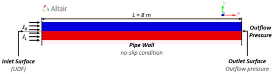
Figure 1.
Representation of fluid domain in Altair AcuSolve and the applied boundary conditions.
Initially, the piping was filled with stratified two-phase flow with 50% liquid holdup. A user-defined function was then incorporated at the inlet surface boundary to impose perturbations. The volume fraction of the liquid phase was set as a function of time:
The pipe and fluid domain mesh are shown in Figure 2. A fine mesh was placed at the fluid–internal pipe surface interface so that the fluid behaviour and the slug effect on the pipe surface could be accurately observed and determined. The maximum absolute cell length was 2 mm with an aspect ratio of 1.63 and maximum skewness angle of 37.4°.
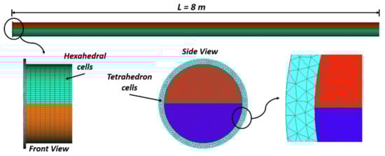
Figure 2.
Mesh operation with front and side view of piping geometry.
Mesh independence study was carried out by varying the number of cells. The number of cells was varied to optimise the number of cells and to ensure that mesh independence was reached. As shown in Figure 3, increasing the number of elements to more than 388,504 resulted in a 0.5% change in the slug frequency values. Therefore, we set the optimum number of elements in this study to 388,504.
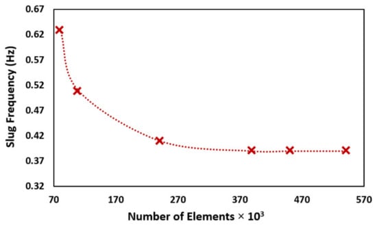
Figure 3.
Mesh independence study for developed CFD model using Altair AcuSolve.
2.3. Mathematical Formulation of Solid Domain
An explicit dynamic solver was employed for the finite element (FE) model, which utilises the widely used Newmark integration scheme for the structural response analysis to determine the induced stresses caused by the slug flow. The explicit finite element equation of motion is expressed as
where M, C and K are constant values that represent the mass matrix, damping matrix and stiffness matrix, respectively; q represents the coordinates used in the mechanical system configuration; F is the load vector at the t th time step; and are the acceleration, velocity and displacement, respectively.
The solution was derived through a one-step time integration by solving the equation of motion in the Newmark scheme. The results were formulated in terms of time history. The vector iterations were calculated through the following system:
where and are the acceleration, velocity and initial displacement, respectively. The resultant load at time t was determined by
The displacement at time was calculated using the following expression:
The dynamic stress at time can be predicted from the displacement at time through the following expression:
The Young’s modulus, Poisson’s ratio and stain displacement matrix are denoted by , and , respectively.
2.4. Solid Model
The developed model was validated against the experimental measurement of Mohmmed []. The developed solid model’s material properties which are similar to the Plexiglass piping specifications of [], are listed in Table 1.

Table 1.
FEA model’s piping geometry and physical properties.
Figure 4 shows that fixed support boundary conditions were adopted at the inlet and outlet surfaces to simulate the operating conditions of the experimental work of Mohmmed []. The resultant pressure profile from the fluid model domain was extracted from the CFD simulation and mapped in the solid structure.
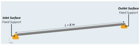
Figure 4.
Representation of solid domain in Altair OptiStruct and the applied boundary condition.
A mesh independence study of the solid model was conducted. The number of elements was varied, as shown in Figure 5. Increasing the number of elements to more than 86,880 resulted in a 0.21% change in the value of the maximum induced stresses predicted by the present model. Therefore, the optimum number of elements of 86,880 was used in the present FSI model.
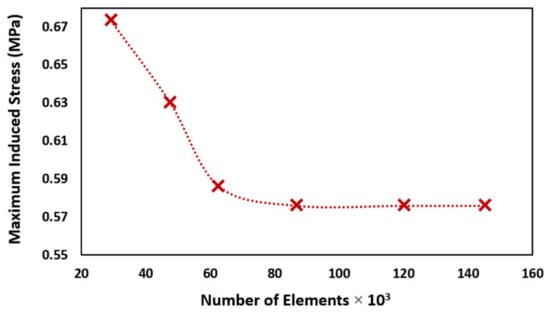
Figure 5.
Mesh independence study for developed FE model using Altair OptiStruct.
The developed model showed a 10% variation against the experimental measurement of Mohmmed []; hence, the results of both works could be considered to have a reasonable agreement. The developed model could thus be used to predict the induced stresses in carbon steel ASTM SA106 Grade B pipes, which are widely used in oil and gas plants.
3. Results and Discussion
This section is divided into two parts, namely, CFD modelling and solid modelling. As mentioned previously, Altair AcuSolve and Altair OptiStruct are respectively used in the CFD modelling for the fluid domain and the solid modelling for the one-way coupled FSI.
3.1. Numerical Model Validation
As mentioned, this research investigates varying crude oil grade effect on slug characteristics and induced stresses. Due to the fact, and to the authors best knowledge, there is no published research that investigates the effect of crude oil slug flow on induced stresses in horizontal pipes. Hence the results of ‘water-air’ slug flow published by [] was used to validate this model which could be considered as reasonably acceptable validation; taking into consideration that the software solvers (CFD and FE) used in this research solve the same governing equations for both crude oil–natural gas and ‘water-air’ multiphase flow. Past research also performed their validation and verification models of crude oil against ‘water-air’ multiphase published results [,].
3.1.1. CFD Fluid Domain Model Validation
The developed CFD model was further validated quantitatively by comparing the results of the predicted slug characteristics (slug initiation position, slug translational velocity, slug liquid length and slug frequency) for the cases shown in Table 2 with the measured results by Mohmmed []. Selected cases (1, 2 and 4) were used to validate qualitatively the present model with the slug contours of the STAR-CCM+ model and slug images from Mohmmed [].
Table 2.
Cases for the quantitative validation of CFD model.
The results of the qualitative analysis of slug formation and growth and the liquid length of the present model were compared with the slug contours in the experimental work and numerical model of Mohmmed [] (Figure 6). The captured slugs present different hydrodynamic behaviours and liquid lengths, which change as a function of gas and liquid superficial velocities. The slug flow for jL = 1 m/s and jG = 2.44 m/s shows the shortest liquid slug which increases in length as the water superficial velocity decreases, as in jL = 0.86 m/s and jL = 0.7 m/s. As shown in Figure 6, the qualitative results of the developed CFD model are in good agreement with those of the experimental work and CFD model of Mohmmed [].
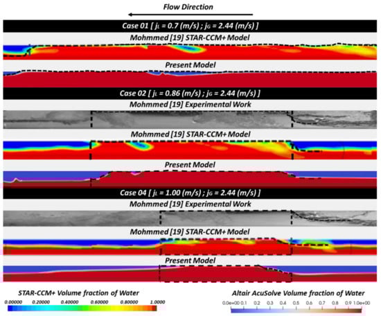
Figure 6.
Qualitative validation of slug contours against the experimental work and numerical model of Mohmmed [].
Figure 7 shows the quantitative validation of slug initiation position, slug translational velocity, slug liquid length and slug frequency against those reported by Mohmmed []. In general, the slug characteristics are strongly dependent on the water and air superficial velocities. As the water superficial velocity increases, the slug formation tends to occur further downstream from the piping inlet. Moreover, a reduction in the slug liquid length is observed as the water superficial velocity increases. The comparison of the results of the present model with those of Mohmmed [] shows that the highest deviations recorded for the slug initiation position, slug translational velocity, slug liquid length and slug frequency are 11.8%, 11.5%, 10.8% and 11.8%, respectively. Mohmmed [] validated his experimental work by using the STAR-CCM+ numerical model [] and found that the highest deviation recorded for slug length was 17.6% when jG = 2.44 m/s and jL = 0.86 m/s. Therefore, relative to the experimental work of Mohmmed [], the present model achieves a reasonable prediction of slug characteristics.
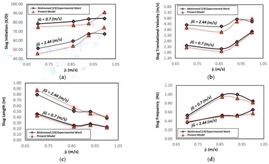
Figure 7.
Quantitative validation of air–water two-phase flow in the present model against the experimental work of Mohmmed []. Validation of (a) slug initiation position; (b) slug translational velocity; (c) slug liquid length; (d) slug frequency.
3.1.2. FSI Model Validation
The maximum induced stresses due to the effect of the slug flow characteristics on the piping were used to validate the FSI model in the current work. Cases 1, 2 and 4 from the CFD model were utilised for the FSI model validation, and the results were compared against the findings of Mohmmed []. Figure 8 illustrates the maximum induced stresses plotted against the water superficial velocity and the quantitative comparison.
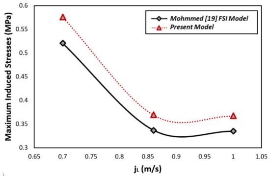
Figure 8.
Quantitative validation of maximum induced stresses due to the effect of the slug characteristics of the air–water two-phase flow validation cases and comparison of FSI model of the present study against the FSI model of Mohmmed [].
Through the comparison of the results from the present model with those by Mohmmed [], the deviations for Cases 1, 2 and 4 are recorded as 9.5%, 8.7% and 8.8%, respectively. The deviations indicate the reasonable agreement of the results compared.
3.2. Effect of Varying Crude Oil Grades on Slug Characteristics
After performing the validation, the model was modified to include the effect of varying the crude oil grade (density and viscosity) on the slug characteristics in the carbon steel pipe. Table 3 lists the properties of the natural gas–crude oil two-phase flow and the modelled cases’ superficial velocities. In practical applications, the oil superficial velocity lies in the range of 0.1–1 m/s whilst the natural gas superficial velocity lies between 0.5 and 4 m/s []; these values explain the selection of the cases under investigation herein.
Table 3.
Physical properties of two-phase flow.
3.2.1. Slug Initiation Position
Figure 9 illustrates the slug initiation position for the modelled cases. Under the constant superficial velocities of gas and crude oil, an increase in crude oil density causes the slug initiation position to decrease. Moreover, the slug initiation position for light crude oil increases by 25% when the liquid velocity increases at a constant gas velocity jG = 2.44 (m/s). As the density of crude oil increases, the location of the slug initiation position moves closer to the inlet and decreases by 84% for very heavy crude oil, 48% for the heavy crude oil and 16% for medium crude oil relative to light crude oil.
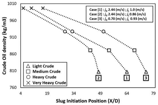
Figure 9.
Effect of varying crude oil grades on slug initiation position (‘D’ represents the pipe diameter).
Figure 9 also shows that the variation in slug initiation position is minimal when the crude oil grade increases and is highly noticeable for light crude oil. Meanwhile, decreasing the gas velocity to 0.7 m/s at 0.93 m/s liquid velocity results in a noticeable increase in slug initiation position for light-grade crude oil; this increase is minimal for very heavy crude oil. The contours shown in Figure 10 indicate that for light crude oil (low-viscosity crude oil), the slug initiation occurs further toward the downstream distance. As the crude oil grade increases at a constant gas–liquid velocity, the slug formation occurs close to the pipe inlet.
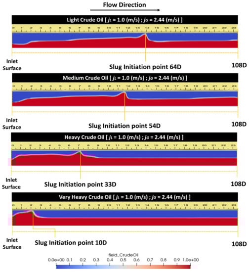
Figure 10.
Effect of varying crude oil grades on slug initiation position (‘D’ represents the pipe diameter).
Figure 11 shows that for light crude oil, 1 m/s liquid superficial velocity results in a stratified wavy flow pattern prior to slug formation. Slug formation occurs closer to the inlet under a lower liquid velocity (0.86 m/s) than under the 1 m/s liquid velocity. At jL = 0.86 m/s and jL = 1 m/s, the slug is captured at 48D and 64D from the inlet surface, respectively. When the gas velocity drops to jG = 0.7 (m/s) at jL = 0.93 (m/s), the maximum initiation position is captured for the light crude oil at 75D; this position is farther than the slug positions for Cases 1 and 2.
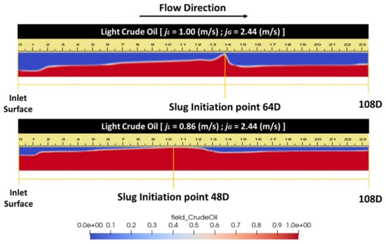
Figure 11.
Effect of varying liquid superficial velocities on slug initiation position (‘D’ represents pipe diameter).
3.2.2. Slug Liquid Length
Slug liquid length is one of the main characteristics of slug flow, and an incorrect prediction may cause flooding in the downstream equipment and thereby result in production deferment. Figure 12 illustrates the effect of changing the oil grades on the slug liquid length. For all investigated cases, increasing the crude oil density decreases the slug length.
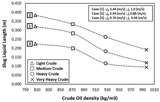
Figure 12.
Effect of varying crude oil grades on slug liquid length.
Moreover, decreasing the liquid velocity at a constant gas velocity causes an increase in slug length. By contrast, up to 30% decrease in slug length is recorded when the gas velocity decreases at liquid velocity of 0.93 m/s as compared with Case 1.
3.2.3. Slug Translational Velocity
The effect of varying crude oil grades on slug translational velocity is presented in Figure 13. The slug translational velocity for high-density crude oil is higher than that for low-density oil. This difference can be explained by considering the mass per unit volume of liquid slug. As shown in Figure 12, higher density crude oil has shorter slug length. Although the slug length decreases, the decrease is larger than the increase in oil density. Hence the mass of the slug for higher density oil is less than the mass of lower oil density which causes the slug translation velocity to increase.
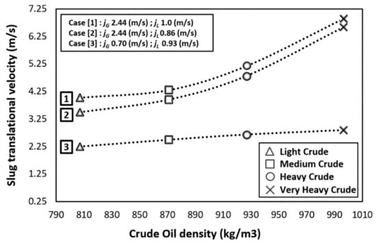
Figure 13.
Effect of varying crude oil grades on slug translational velocity.
The variation of velocity with respect to crude oil grade is minimal at a low gas velocity at 0.93 m/s liquid velocity. However, the increase in slug velocity becomes increasingly noticeable when the liquid velocity increases from 0.86 to 1 m/s at 2.44 m/s gas velocity.
3.2.4. Slug Frequency
Figure 14 illustrates the effect of varying crude oil grades on slug frequency.
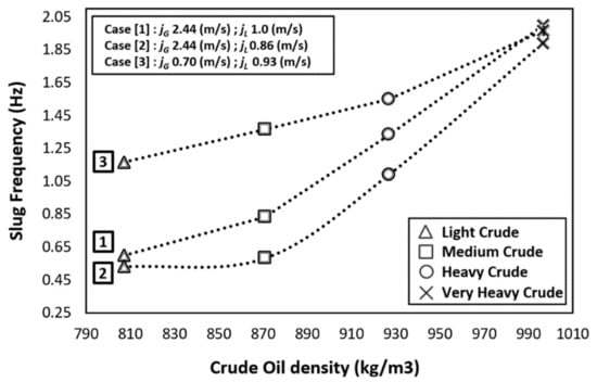
Figure 14.
Effect of varying crude oil grades on slug frequency.
The slug frequency increases when the crude oil density increases. Moreover, as the density of crude oil increases, the difference in slug frequency values decreases at different fluid and gas velocities. For instance, the slug frequency for very heavy crude oil fluctuates between 1.89 and 2 Hz for all examined superficial velocities.
For light crude oil, the slug frequency is highly influenced by the superficial velocity of the gas and liquid phases, and the variation is more noticeable than that of heavy crude oil. When the gas and liquid superficial velocities are 0.7 and 0.93 m/s, respectively, the slug frequency for light crude oil is 1.17 Hz. As the gas and liquid superficial velocities increase to 2.44 and 1.0 m/s, respectively, the slug frequency noticeably decreases to 0.6 Hz. By maintaining the gas phase superficial velocity at 2.44 m/s and decreasing the crude oil superficial velocity to 0.86 m/s, the slug frequency further decreases to 0.53 Hz.
3.3. Effect of Varying Crude Oil Grades on Maximum Induced Stresses
Slug flow occurrence is known to cause serious damage to pipelines. Hence, the effect of slug characteristics on induced stresses in carbon steel pipes is investigated in this work. Figure 15 shows that varying crude oil grades cause significant variation in maximum induced stresses values. The flow of light crude oil records the lowest induced stresses. However, as the crude oil density increases, the induced stresses increase.
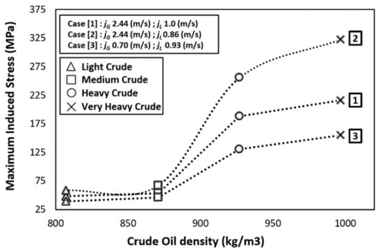
Figure 15.
Effect of varying crude oil grades on maximum induced stresses.
Figure 15 also shows that the flow of light and medium crude oil in carbon steel pipe records a marginal increase in stresses when the liquid and gas velocities change. By contrast, when heavy and extra heavy crude oil flow in pipes, the margin of increase in induced stresses due to changes in gas and liquid velocities is significant.
Moreover, for very heavy crude oil, the maximum induced stresses decrease by up to 33% when the liquid velocity increases at a constant gas velocity. Meanwhile, decreasing the gas velocity at 0.93 m/s liquid velocity records the lowest induced stresses for all crude oil grades.
The slug initiation position is a function of the operating conditions and physical properties of flowing media. Slug formation in piping systems subsequently exerts hydrodynamic loads on the piping’s inner surface. The perturbation of the slug that moves with a velocity higher than the gas and liquid superficial velocities causes high momentum, which is then transferred to the piping wall where it causes induced stresses.
Figure 16 illustrates the relation between the slug initiation position and the induced stresses for Case 1. As the slug formation occurs at 64D (D represents the pipe diameter) for the light crude oil, the maximum induced stress observed is 48 MPa at the location of slug formation. When the crude oil density increases, the liquid slug translational velocity increases (Figure 13), thereby causing the slug to move with high momentum. This condition leads to high induced stresses, as seen in the medium crude, heavy and very heavy crude oil grades with maximum recorded induced stresses of 54, 189 and 216 MPa, respectively, as shown in Figure 16.
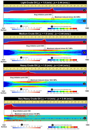
Figure 16.
Effect of slug hydrodynamics (A) on the maximum induced stresses (B) (‘D’ represents pipe diameter).
Slug liquid length is one of the main variables that characterise slug flow and could be associated with maximum induced stresses when the liquid impinges on the internal wall of the pipe. Thus, the relationship between slug length and maximum induced stresses for various crude oil grades should be understood.
Figure 17 shows that for all cases (Cases 1, 2 and 3), when the slug length increases, the recorded maximum induced stresses decrease. For heavy and extra heavy crude oil at a constant gas velocity, increasing the liquid velocity causes a decrease in slug length and consequently leads to high stresses. A possible reason is that the stresses are related to both the magnitude of force and the area. Hence, the induced stresses caused by the slug flow is affected by the fluid density and mass of the slug and the size of the crude oil slug impinged area at the pipe surface.
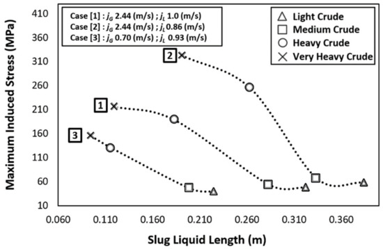
Figure 17.
Effect of slug liquid length on maximum induced stresses.
However, decreasing the gas velocity to 0.7 m/s at 0.93 m/s liquid velocity records the lowest induced stresses for all investigated cases. It is important to mention that this research mainly investigates varying the liquid velocity at constant gas velocity.
The results of the induced stresses indicate the need to carefully perform pipeline designs that handle heavy and extra heavy crude oil because the maximum induced stresses may change significantly after a slight change in liquid superficial velocities. Moreover, when the slug moves at a velocity that is higher than the gas and liquid superficial velocities, the slug moves with higher momentum, resulting in higher maximum induced stresses.
4. Conclusions
The effect of varying crude oil densities on slug characteristics and consequently on induced stresses was numerically investigated using gas–crude oil two-phase flow in a horizontal carbon steel pipe.
The variation of crude oil properties exerts a significant effect on the slug characteristics of the various cases investigated.
For light crude oil, a 14% decrease in slug translational velocity, 16% decrease in slug length and 13% increase in slug frequency are recorded when the liquid superficial velocity increases at a constant gas velocity. Moreover, increasing the crude oil density results in an increase in maximum induced stresses. Meanwhile, varying liquid and gas velocities causes a small variation in maximum induced stresses when light and medium crude oil are modelled. When heavy and extra heavy crude oil are modelled, the variation in induced stresses is significant. Hence, when flow operating conditions change, the design of pipelines that handle heavy and extra heavy crude oil should be carefully performed because small variations in liquid flow velocity may cause significant changes in maximum slug-induced stresses.
Author Contributions
Conceptualisation, M.E., M.S.N. and M.M.; methodology, M.E. and M.S.N.; software, M.E. and M.S.N.; validation, M.E. and M.S.N.; formal analysis, M.E. and M.S.N.; investigation, M.E. and M.S.N.; resources, M.S.N.; data curation, M.E.; writing—original draft preparation, M.E.; writing—review and editing, M.S.N.; visualisation, M.E.; supervision, M.S.N. and M.M.; project administration, M.S.N. funding acquisition, M.S.N. All authors have read and agreed to the published version of the manuscript.
Funding
The authors acknowledge the financial support provided by Universiti Teknologi PETRONAS through Yayasan Universiti Teknologi PETRONAS grant (YUTP 015LC0-159) to publish this research.
Institutional Review Board Statement
Not applicable.
Informed Consent Statement
Not applicable.
Data Availability Statement
The data presented in this study are available on request from the corresponding authors. The data are not publicly available due to privacy.
Acknowledgments
The authors wish to acknowledge the support of Universiti Teknologi PETRONAS for providing the resources to support this research.
Conflicts of Interest
The authors declare no conflict of interest.
References
- Liu, G.; Hao, Z.; Wang, Y.; Ren, W. Research on the Dynamic Responses of Simply Supported Horizontal Pipes Conveying Gas-Liquid Two-Phase Slug Flow. Processes 2021, 9, 83. [Google Scholar] [CrossRef]
- O’Neill, L.E.; Mudawar, I. Review of two-phase flow instabilities in macro- and micro-channel systems. Int. J. Heat Mass Transf. 2020, 157, 119738. [Google Scholar] [CrossRef]
- Wang, B.; Shen, S.; Ruan, Y.; Cheng, S.; Peng, W.; Zhang, J. Simulation of Gas-Liquid Two-Phase Flow in Metallurgical Process. Acta Metall. Sin. 2020, 56, 619–632. [Google Scholar] [CrossRef]
- Wu, B.; Firouzi, M.; Mitchell, T.; Ru_ord, T.E.; Leonardi, C.; Towler, B. A critical review of flow maps for gas-liquid flows in vertical pipes and annuli. Chem. Eng. J. 2017, 326, 350–377. [Google Scholar] [CrossRef]
- Risso, F. Agitation, Mixing, and Transfers Induced by Bubbles. Annu. Rev. Fluid Mech. 2018, 50, 25–48. [Google Scholar] [CrossRef]
- Nnabuife, S.G.; Sharma, P.; Iyore Aburime, E.; Lokidor, P.L.; Bello, A. Development of Gas-Liquid Slug Flow Measurement Using Continuous-Wave Doppler Ultrasound and Bandpass Power Spectral Density. ChemEngineering 2021, 5, 2. [Google Scholar] [CrossRef]
- Sergeev, V.; Vatin, N.; Kotov, E.; Nemova, D.; Khorobrov, S. Slug Regime Transitions in a Two-Phase Flow in Horizontal Round Pipe. CFD Simulations. Appl. Sci. 2020, 10, 8739. [Google Scholar] [CrossRef]
- Lin, P.Y.; Hanratty, T.J. Prediction of the initiation of slugs with the linear stability theory. Int. J. Multiph. Flow 1987, 12, 79–98. [Google Scholar] [CrossRef]
- Woods, B.D.; Fan, Z.; Hanratty, T.J. Frequency and development of slugs in a horizontal pipe at large liquid flows. Int. J. Multiph. Flow 2006, 32, 902–925. [Google Scholar] [CrossRef]
- Dafyak, L.; Appah, D.; Onuoha, S.; Mukhtar, A. Effect of pipe inclination on the hydrodynamics of slug flow. In Proceedings of the SPE Nigeria Annual International Conference and Exhibition, Lagos, Nigeria, 6–8 August 2018. [Google Scholar] [CrossRef]
- Shen, R.; Jiao, Z.; Parker, T.; Sun, Y.; Wang, Q. Recent application of Computational Fluid Dynamics (CFD) in process safety and loss prevention: A review. J. Loss Prev. Process Ind. 2020, 67, 104252. [Google Scholar] [CrossRef]
- Frank, T. Numerical simulation of slug flow regime for an air-water two-phase flow in horizontal pipes. In Proceedings of the 11th International Topical Meeting on Nuclear Reactor Thermal-Hydraulics (NURETH-11), Avignon, France, 2–6 October 2005. [Google Scholar]
- Lex, T. Beschreibung Eines Testfalls zur Horizontalen Gas-Flüssigkeitsströmung; Technische Universität München: Munich, Germany, 2003. [Google Scholar]
- Woods, B.D.; Hanratty, T.J. Influence of Froude number on physical processes determining frequency of slugging in horizontal gas–liquid flows. Int. J. Multiph. Flow 1999, 25, 1195–1223. [Google Scholar] [CrossRef]
- Adibi, P.; Ansari, M.; Jafari, S.; Habibpour, B.; Salimi, E. Slug Initiation Evaluation in Long Horizontal Channels Experimentally. Int. J. Mech. Aerosp. Ind. Mechatron. Manuf. Eng. 2014, 8, 92–98. [Google Scholar] [CrossRef]
- Xu, K.; Zhang, Y.; Liu, D.; Azman, A.N.; Kim, H. Slug flow development study in a horizontal pipe using particle image velocimetry. Int. J. Heat Mass Transf. 2020, 162, 120267. [Google Scholar] [CrossRef]
- Doyle, B.J.; Morin, F.; Haelssig, J.B.; Roberge, D.M.; Macchi, A. Gas-Liquid Flow and Interphase Mass Transfer in LL Microreactors. Fluids 2020, 5, 223. [Google Scholar] [CrossRef]
- Mohmmed, A.O.; Nasif, M.S.; Al-Kayiem, H.H. Numerical investigation of slug characteristics in a horizontal air/water and air/oil pipe flow. Prog. Comput. Fluid Dyn. 2018, 18, 241–256. [Google Scholar] [CrossRef]
- Mohmmed, A.O.I. Effect of Slug Two-Phase Flow on Fatigue of Pipe Material. Ph.D. Thesis, Universiti Teknologi PETRONAS, Perak, Malaysia, June 2016. [Google Scholar]
- Sam, B.; Pao, W.; Nasif, M.S. Numerical simulation of two-phase flow regime in horizontal pipeline and its validation. Int. J. Numer. Methods Heat Fluid Flow 2018, 8, 1279–1314. [Google Scholar] [CrossRef]
- Pao, W.; Sam, B.; Nasif, M.S.; Norpiah, F.M. Numerical validation of two-phase slug flow and its liquid holdup correlation in horizontal pipeline. Key Eng. Mater. 2016, 740, 173–182. [Google Scholar] [CrossRef]
- Losi, G.; Arnone, D.; Correra, S.; Poesio, P. Modelling and statistical analysis of high viscosity oil/air slug flow characteristics in a small diameter horizontal pipe. Chem. Eng. Sci. 2016, 148, 190–202. [Google Scholar] [CrossRef]
- Baba, Y.D.; Aliyu, A.M.; Archibong, A.E.; Abdulkadir, M.; Lao, L.; Yeung, H. Slug length for high viscosity oil-gas flow in horizontal pipes: Experiments and prediction. J. Pet. Sci. Eng. 2018, 165, 397–411. [Google Scholar] [CrossRef]
- Baba, Y.D.; Archibong-Eso, A.; Aliyu, A.M.; Fajemidupe, O.T.; Ribeiro, J.X.F.; Lao, L.; Yeung, H. Slug translational velocity for highly viscous oil and gas flows in horizontal pipes. Fluids 2019, 4, 170. [Google Scholar] [CrossRef]
- Shadloo, M.; Rahmat, A.; Karimipour, A.; Wongwises, S. Estimation of Pressure Drop of Two-Phase Flow in Horizontal Long Pipes Using Artificial Neural Networks. J. Energy Resour. Technol. 2020, 142, 1–21. [Google Scholar] [CrossRef]
- Abdulkadir, M.; Hernandez-Perez, V.; Lowndes, I.S.; Azzopardi, B.J.; Sam-Mbomah, E. Experimental study of the hydrodynamic behavior of slug flow in a horizontal pipe. Chem. Eng. Sci. 2016, 156, 147–161. [Google Scholar] [CrossRef]
- Reda, M.; Forbes, G.L.; Sultan, I.A. Characterization of slug flow conditions in pipelines for fatigue analysis. In Proceedings of the ASME 2011 30th International Conference on Ocean, Offshore and Arctic Engineering (OMAE2011), Rotterdam, The Netherlands, 19–24 June 2011. [Google Scholar]
- Kansao, R.; Casanova, E.; Blanco, A.; Kenyery, F.; Rivero, M. Fatigue life prediction due to slug flow in extra-long submarine gas pipelines. In Proceedings of the ASME 2008 27th International Conference on Offshore Mechanics and Arctic Engineering (OMAE2008), Estoril, Portugal, 15–20 June 2008. [Google Scholar]
- Van der Heijden, B.H.E.J.; Semienk, H.; Metrikine, A.V. Fatigue Analysis of subsea jumper due to slug flow. In Proceedings of the ASME 2014 33rd International Conference on Ocean, Offshore and Arctic Engineering (OMAE2014), San Francisco, CA, USA, 8–13 June 2014. [Google Scholar]
- Chica, L.; Pascali, R.; Jukes, P.; Ozturk, B.; Gamino, M.; Smith, K. Detailed FSI analysis methodology for subsea piping components. In Proceedings of the ASME 2012 31st International Conference on Ocean, Offshore and Arctic Engineering (OMAE2012), Rio de Janeiro, Brazil, 1–6 July 2012. [Google Scholar]
- An, C.; Su, J. Dynamic behaviour of pipes conveying gas-liquid two-phase flow. Nucl. Eng. Des. 2015, 292, 204–212. [Google Scholar] [CrossRef]
- Wang, L.; Yang, Y.; Li, Y.; Wang, Y. Dynamic behaviours of horizontal gas-liquid pipes subjected to hydrodynamic slug flow: Modelling and experiments. Int. J. Press. Vessel. Pip. 2018, 161, 50–57. [Google Scholar] [CrossRef]
- Mohmmed, A.O.; Al-Kayiem, H.H.; Nasif, M.S.; Time, R.W. Effect of slug flow frequency on the mechanical stress behaviour of pipelines. Int. J. Press. Vessel. Pip. 2019, 172, 1–9. [Google Scholar] [CrossRef]
- Almutairi, Z.; Al-Alweet, F.M.; Alghamdi, Y.A.; Almisned, O.A.; Alothman, O.Y. Investigating the Characteristics of Two-Phase Flow Using Electrical Capacitance Tomography (ECT) for Three Pipe Orientations. Processes 2020, 8, 51. [Google Scholar] [CrossRef]
- Xu, Z.; Wu, F.; Yang, X.; Li, Y. Measurement of Gas-Oil Two-Phase Flow Patterns by Using CNN Algorithm Based on Dual ECT Sensors with Venturi Tube. Sensors 2020, 20, 1200. [Google Scholar] [CrossRef]
- Roshani, M.; Phan, G.T.T.; Ali, P.J.M.; Roshani, G.; Hanus, R.; Duong, T.; Corniani, E.; Nazemi, E.; Kalmoun, E. Evaluation of flow pattern recognition and void fraction measurement in two phase flow independent of oil pipeline’s scale layer thickness. Alex. Eng. J. 2021, 60, 1955–1966. [Google Scholar] [CrossRef]
- Roshani, M.; Phan, G.; Roshani, G.; Hanus, R.; Nazemi, B.; Corniani, E.; Nazemi, E. Combination of X-ray tube and GMDH neural network as a nondestructive and potential technique for measuring characteristics of gas-oil–water three phase flows. Measurement 2021, 168, 108427. [Google Scholar] [CrossRef]
- Fang, L.; Zeng, Q.; Wang, F.; Faraj, Y.; Zhao, Y.; Lang, Y.; Wei, Z. Identification of two-phase flow regime using ultrasonic phased array. Flow Meas. Instrum. 2020, 72, 101726. [Google Scholar] [CrossRef]
- Hu, L.; Li, Y. A limiting strategy for the back and forth error compensation and correction method for solving advection equations. Math. Comput. 2016, 85, 1263–1280. [Google Scholar] [CrossRef]
- Kim, B.M.; Liu, Y.J.; Llamas, I.; Rossignac, J.R. FlowFixture: Using BFECC for fluid simulation. In Proceedings of the Eurographics Workshop on Natural Penomena, Dublin, Ireland, 30 August 2005. [Google Scholar]
- He, X.; Wang, H.; Zhang, F.; Wang, H.; Wang, G.; Zhou, K.; Wu, E. Simulation of fluid mixing with interface control. In Proceedings of the 14th ACM SIGGRAPH/Eurographics Symposium on Computer Animation, Los Angeles, CA, USA, 7–9 August 2015. [Google Scholar]
- Sussman, M.; Smereka, P.; Osher, S. A level set approach for computing solutions to incompressible two-phase flow. J. Comput. Phys. 1994, 114, 146–159. [Google Scholar] [CrossRef]
- Herrmann, M. A balanced force refined level set grid method for two-phase flows on unstructured flow solver grids. J. Comput. Phys. 2008, 227, 2674–2706. [Google Scholar] [CrossRef]
- Akhiyarov, D.T.; Zhang, H.Q.; Sarica, C. High-viscosity oil-gas flow in vertical pipe. In Proceedings of the 2010 Offshore Technology Conference, Houston, TX, USA, 3–6 May 2010. [Google Scholar]
Publisher’s Note: MDPI stays neutral with regard to jurisdictional claims in published maps and institutional affiliations. |
© 2021 by the authors. Licensee MDPI, Basel, Switzerland. This article is an open access article distributed under the terms and conditions of the Creative Commons Attribution (CC BY) license (https://creativecommons.org/licenses/by/4.0/).