Cationic and Anionic Dye Adsorption on a Natural Clayey Composite

Abstract

One of the main challenges for environmental sciences today is the effective treatment of dye-laden industrial effluents. This work aimed to study the potential of an untreated (natural occurring clayey composite) red clay (RC) for the adsorption of a cationic dye Basic Navy Blue 2RN (CNB) and anionic dye Drimaren Yellow CL-2R (ADY). We evaluated the effect of pH, dye concentration, and adsorbent concentration on the removal effectiveness to study the absorption process. Also, we studied the adsorption process by analyzing the feasibility of several known adsorption isotherms and kinetic models. The results show that at a pH of less than 4, the CNB and ADY removal percentages were 97% and 96%, respectively. At a pH greater than 8, the CNB and ADY removals were 75% and 25%, respectively. The CNB adsorption happened by chemisorption of a monolayer on iron-containing particles (IPs). In congtrast, the ADY adsorption occurred by monolayer physisorption on kaolinite particles (KPs) and Na, K-rich Laumontite particles (LPs). The Langmuir isotherm model fits very well with CNB experimental data. The Temkin model shows the best fit between the isotherm function and the ADY dye-adsorption data. The pseudo-second-order kinetic model fits the CNB and ADY dye-adsorption data on RC particles. The heterogeneous composition of naturally occurring clay favors different adsorption mechanisms and opens an avenue for the separation process’s engineering.

1. Introduction

The agricultural and industrial sectors consume 70% and 22% of the available freshwater, respectively. This consumption results in large amounts of wastewater [1] and leads to worldwide freshwater availability changes [2]. In particular, dyes’ discharge to effluents can reach up to 50% of the initially used amount in the textile industry, depending on substrate and dye type [3]. Dyes’ discharge to effluents and climate variation, among other issues, are emerging threats to water and food [2,4] that have endangered the equilibrium of natural ecosystems. Dyes are recalcitrant organic molecules, resistant to aerobic digestion, and stable to light, heat, and oxidizing agents [5]. Because of dyes’ potential toxicity to human health, many have been classified as hazardous pollutants [6]. Dyes potentially alter the genetic constitution by changing the deoxyribonucleic acid (DNA). They are considered to be mutagenic and genotoxic chemical agents. Therefore, the discharge of dyes on water bodies is a significant environmental contamination source [4,7]. Dyes tend to sequester metal and may cause microtoxicity to fish and other organisms [1]. At present, around 100,000 dyes exist and are toxic beyond the threshold level. This number is gradually increasing and constitutes a threat to the biosphere. As such, it is crucial to treat colored effluents for the removal of dyes [8].

Dyes organic compounds are based on functional groups such as the chromophore group (NR₂, NHR, NH₂, COOH, and OH) and auxochromes (N₂, NO, and NO₂) [3]. There are different dyes: acid, basic, disperse, direct, reactive, solvent, sulfur, and vat dyes, amount others [1,3]. Several treatment methods have been developed to treat colored effluents: biological treatment, membrane separation, chemical oxidative processes, electrochemical processes, and adsorption processes [9]. However, one factor to consider within the existing alternatives is the treatments’ high investment and operating costs, energy expenditure, and the waste generated [10]. The adsorption process is a promising technique to treat wastewater, which utilizes natural materials as an adsorbent. It is regarded as eco-friendly and economical to operate. The adsorbent in the highest demand is activated carbon, due to its adsorption capacity [11], because of its large specific surface area [12]. However, active carbon has some drawbacks, primarily related to its high cost and complicated regeneration process [13]. Alternatively, dye removal by clay has shown promising results. Clays are suitable adsorbent materials for the adsorption of various pollutants because of their: high surface area, porosity, thermal stability, specific active sites, high cation exchange capacity, easy availability, and attractive adsorptive properties [14].

Clay refers to a material that: (1) occurs naturally on the earth’s surface, (2) is composed primarily of colloidal grains of minerals, (3) forms a viscous, plastic mass when mixed with water, and (4) hardens and holds its shape when dried or baked. The natural–pristine clays’ constituents are mineral clays and associated minerals. Mineral clay provides plasticity, e.g., kaolinite, montmorillonite, illite, and vermiculite. It hardens when dried or fired. The associated minerals do not impart plasticity to clay, e.g., micas, quartz, feldspars, and others: iron oxide; hydroxides such as magnetite, hematite, maghemite, goethite; and aluminum hydroxides such as corundum, gibbsite, boehmite, diaspores. Therefore, natural clays are a mixture of weathered minerals that give rise to unique clayey composite materials. These differences among the clays provide an opportunity to investigate the adsorption potential of these naturally occurring clayey composites as multifunctional adsorbents of pollutants like dyes.

Clays have shown the potential to remove dyes in aqueous solutions [4]. Bentonite removed 88% of acid dyes [15]. Dolomite (CaMg(CO₃)₂) rich natural clay removed 90% of methylene blue [14]. Smectite-rich natural clay removed 80% of acid brow 75 [16]. Natural red clay removed 96% of bright green dye [17]. The adsorption capacity of clays generally results from a net negative charge on the structure of minerals. This negative charge gives clays the capability to adsorb positively charged molecules [18]. Comparatively, clay adsorbents are more cost-effective than active carbon and other organic adsorbents for effluent treatment [3]. Moreover, clay adsorbents reduce costs ten to more times than other adsorbents (

Table 1. The effective cost of effluent treatment with clay and other adsorbents [3].

Adsorbent	USD $/kg	Adsorbent	USD $/kg
Bentonite	0.05–0.3	Active carbon	0.8–1.1
Red mud	0.025	Chitin	15–20
Clinoptilolite	0.14–0.29	Chitosan	16–10
Natural zeolite	0.08	Cross-linked chitosan	5–10

).

Even though many studies deal with clay material as adsorbents, a great deal of work still needs to be done [1,3,19]. There exists a wide variety of dyes, and their removal is based on various factors, which include: adsorbate (dye)–adsorbent (clay) relationships (interactions), adsorbate molecular size, and the role of functional groups on both adsorbate as well as adsorbent. More detailed work on these interactions is needed for the studies to correlate and compare [1].

Composite materials made up of nanomaterial, bio-material, and mineral clay can improve the dye removal effectiveness. However, their cost still hampers practical application. Clayey composites are low-cost adsorbents with unique properties and structural diversity, offering superior performance versus individual clay mineral counterparts. This research aimed to study a clayey composite—naturally occurring red clay—from Ecuador’s Amazonia region as a multifunctional adsorbent to treat dye-laden textile industrial effluents. We selected as adsorbate a cationic dye (Basic Navy Blue 2RN) and an anionic dye (Drimaren Yellow CL-2R) to achieve this objective. We evaluated the effect of pH, adsorbate (dye), and adsorbent (red clay) concentration on the removal effectiveness to study the absorption process. Also, we studied the adsorption process by analyzing the feasibility of several known adsorption isotherms and kinetic models.

2. Materials and Methods

2.1. Materials and Reagents

Archroma (Reinach, Switzerland) provided the CNB dye—Basic Navy Blue 2RN—and the ADY dye—Drimaren Yellow CL-2R—of very high purity (99%), taken as a pollutants model without any prior purification. Chemical and reagents used were of analytical grade, i.e., sulfuric acid (H₂SO₄), sodium chlorite (NaClO₂), HCl, and sodium hydroxide (NaOH) were purchased from Sigma-Aldrich Corp., St Louis, MO, USA. Distilled and de-ionized water was used in all experimental work.

The red clay (RC) samples were collected from a natural deposit at the Province of Pastaza Ecuador (UTM coordinates x = 846,551, y = 9,854,823). Red clay samples were dried at 105 °C for 24 h, mechanically ground in a planetary mill, and reduced to powder in an agate mortar.

2.2. SEM and EDS Characterization

Morphological analysis was performed with the scanning electron microscope (VEGA 3 TESCAM, Kohoutovice, Czech Republic). The sample was fixed in a sample holder using carbon tape (double-sided) and then coated with a thin layer of gold. Energy dispersive spectroscopy of X-ray photon (EDS) was performed to quantify the sample elemental composition. We scan and sample a rectangle area covering the whole image and performed a mapping with quantitative spectrum analysis. The process involved an accurate standardless spectrum analysis based on the P/B-ZAF method.

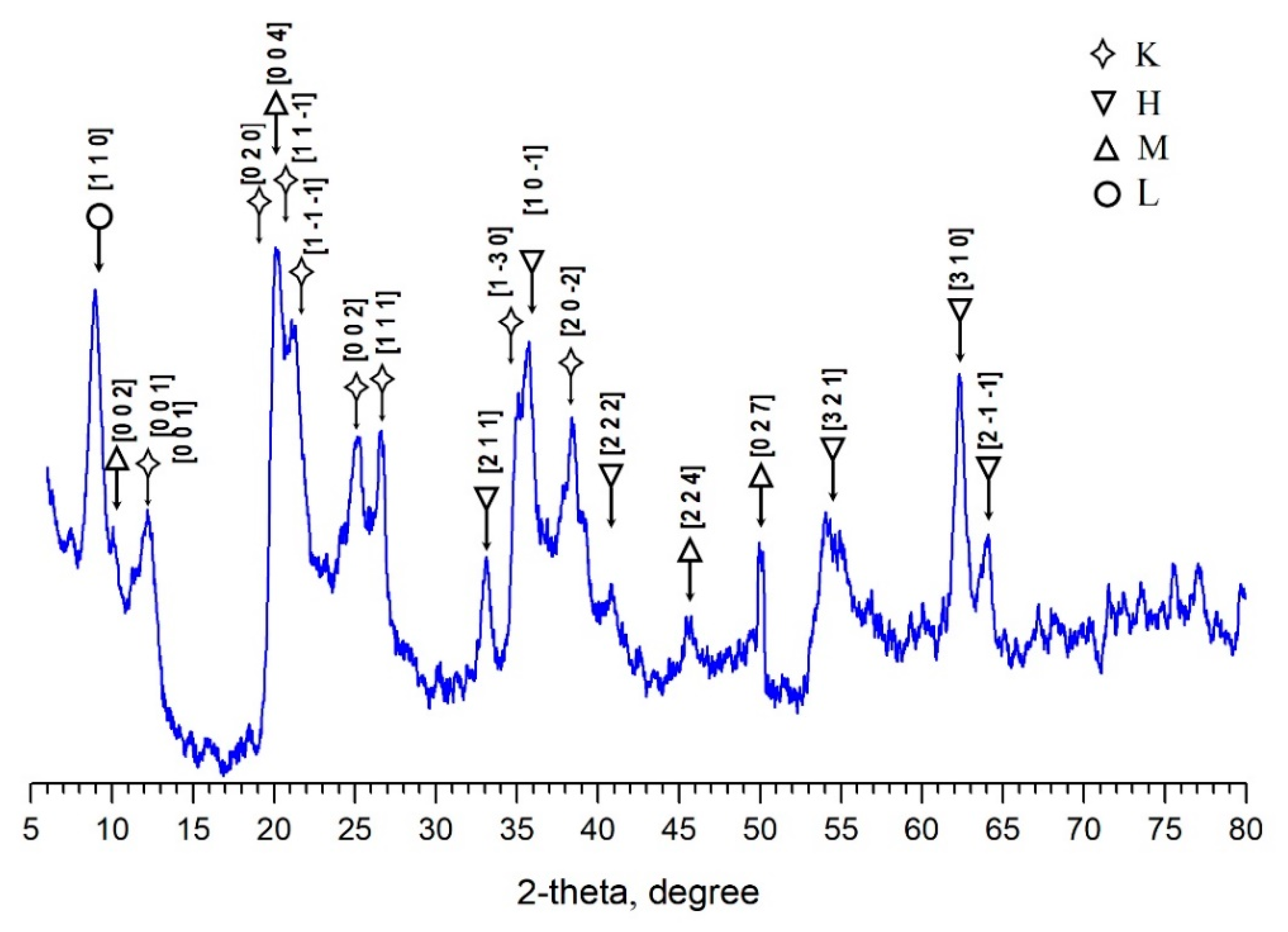
2.3. X-ray Diffraction Characterization

The RC crystalline phases were analyzed via the powder method. We used an X-ray diffractometer (D8 Advance, Bruker, Billerica, MA USA) equipped with a copper anode (λ = 1.5418 Å) and a linear detector (LYNXEYE compound silicon strip detector, Bruker). The diffractograms were collected in a range of 4 to 80 degrees using a step size of 0.02 degrees and a measurement time of 2 s per step. The diffractogram analysis and the qualitative phase analysis were performed using the QualX program [20]. QualX can carry out the phase identification by inquiring about the PDF-2 commercial database and the freely available database: POW_COD. The POW_COD was created by using the structure information contained in the Crystallography Open Database.

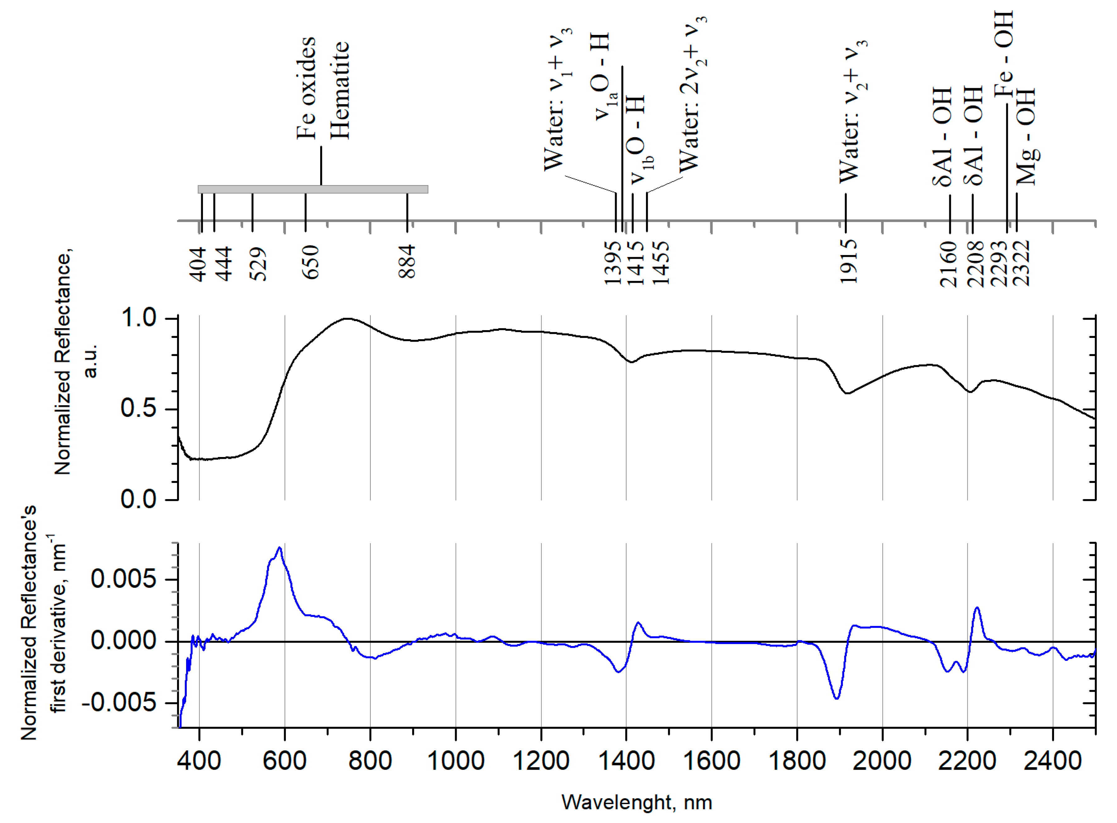
2.4. Vis–NIR Diffused Reflectance Spectroscopy

A portable spectroradiometer (Fieldspec^®4 radiometer, Analytical Spectral Devices Inc., Boulder, CO, USA) was used to record the diffuse reflectance (DR) spectra. The spectroradiometer was used in a proximal mode over the Vis–NIR region (350–2500 nm). The DR spectrum was recorded by illuminating the sample with a 75 W Lowel Pro-Light lamp at 45°. The radiometer’s optic was vertically aligned with the axis passing through the samples’ geometric center. Its height was adjusted so that only light reflected from the materials’ surface filled the instrument’s field of view. A spectralon panel (Labsphere Inc., North Sutton, NH, USA) with 99% reflectance was used as a reference panel (white reference) to optimize the spectroradiometer before taking Vis–NIR reflectance measurements for each sample. The spectroradiometer’s internal configuration consists of three detectors, each collecting spectra from three different spectral regions: 350–1000 nm (Silicon array detector), 1000–1800 nm (InGaAs detector), and 1800–2500 nm (InGaAs detector). The spectra collected by these detectors were not spliced, so each spectrum was corrected, splicing the three aforementioned spectral regions and using the ASD ViewSpec ProTM software (ASD Inc., Boulder, CO, USA). Spectra were recorded consecutively in different angular orientations to eliminate undesirable effects in the spectrum. The spectral was recorded by placing 10 g of the RC in a Petri dish and placed under the lens (3–10 nm, inclination 90°, height 1.5 cm) separated from the sample. Ten spectra were taken (for 4 s) in 4 quadrants (0°,90°, 180°, 270°), obtaining a total of 40 readings for each sample. Spectral reflectance data for each sample were generated by arithmetic averaging four replicated measurements (40 spectra) for that sample. Finally, the readings were normalized to one. We used the Savitzky–Golay algorithm (second-order polynomial and window of 10 wavelengths), implemented in the Origin Lab 9.1 platform (OriginLab Corp., Northampton, MA, USA) to calculate the first derivative of the DR spectra. The DR spectrum first derivative makes feasible spectrum features visualization.

2.5. Adsorption Test

Stock solutions of 1 g/L of CNB and ADY dyes were prepared by dissolving each dye’s appropriated amount in double-distilled water. The used concentrations were obtained by dilution. Adsorption experiments were conducted at room temperature in 50 mL of dyed water in a flask at a constant agitation speed by varying the pH of the solution from 2 to 10, the adsorbent dosage from 0.2 to 1.2 g/50 mL, the contact time from 5 to 60 min, and the initial dye concentration from 15 to 75 mg/L. The pH was adjusted to a given value by adding analytical grade H₂SO₄ (1 N) and NaOH (1 N) reagents. The test solutions were agitated with an IKA shaker, model RT 10 power, IKA^® WERKE (Staufen, Germany). Solutions were agitated at 200 rpm at room temperature (20 °C) for 30 minutes until the adsorption process reached equilibrium. Then, samples were centrifugated with a Thermo Fisher Scientific CL2 centrifuge (Waltham, Massachusetts, USA) at 1000 rpm for 30 minutes to separate the liquid phase and solids. Upon centrifugation, filtration was carried out to separate adsorbents’ filtration and residue with 0.1 μm of membrane filter (Millipore, Japan). The absorbance of the filtrated solution was measured at a wavelength of ${\lambda }_{\mathrm{ADY}}=420\mathrm{nm}$ and ${\lambda }_{\mathrm{CNB}}=650\mathrm{nm}$ with DR 5000 Hach^® UV-visible spectrometer (Loveland, Colorado, USA). The CNB dye shows a peak absorbance at 610 nm. However, the CNB dye optical density was measured at 650 nm to mitigate the azo group hyperchromic effect [21].

The residual dye concentration at the equilibrium state $\left(C_e;\mathrm{mg}/\mathrm{L}\right)$ in the filtrated solution is calculated using Equation (1) upon measuring the calibration curve (optical absorbance vs. dye concentration). The adsorption performance is described by the amount of adsorbate adsorbed or adsorption capacity at equilibrium $\left(q_e;\mathrm{mg}/\mathrm{g}\right)$. Alternatively, the performance is described by the removed adsorbate’s relative amount $\left(\%R\right)$. The adsorption capacity and the percentage of dye removal are calculated using Equations (2) and (3). In these equations, the C_o represents the initial dye concentration expressed in mg/L, V is the label for the total volume of the solution expressed in L, and m represents the absorbent mass in grams. In this study, we carried out three replications of each adsorption experiment.

$$C_e=\frac{\mathrm{Optical}\mathrm{absorption}}{\mathrm{Calibration}\mathrm{constant}}$$

(1)

$$q_e=(C_o-C_e)\left(\frac{V}{m}\right)$$

(2)

$$\%R=\left(1-\frac{C_e}{C_o}\right)\times 100$$

(3)

2.6. Adsorption Isotherm Modeling

The adsorption equilibria data is crucial to understand how much of the adsorbate can fit onto the solid adsorbent surface. The adsorption isotherm models express a mathematical relation between the dye adsorbed and the remained dye concentration in solution. There are many possible interactions between the adsorbent and the adsorbate. Various isotherm models consist of different model parameters [21]. Therefore, we studied the adsorption equilibria data by analyzing the Langmuir, Freundlich, Tempkin, and Dubinin–Radushkevich isotherm models’ feasibility. The criterion for choosing the more feasible isotherm model was that it should be a good fit between the isotherm function and the experimental data. The best-fit isotherm model was determined by carrying out linear regressions of the isotherm linear equation. Data evaluation was accomplished by using R² value analysis.

The Langmuir model (LM) was developed using the following assumptions [22,23,24]: (1) a fixed number of accessible sites are available on the adsorbent surface, and all active sites have the same energy, (2) adsorption is reversible, (3) once the adsorbate occupies a site, no further adsorption can occur on that site (the adsorbate forms a monolayer on the adsorbent surface), and (4) there is no interaction between adsorbate species. The nonlinear and the Lineweaver–Burk linearization of the LM are described in Equation (4). The LM parameters are found when $1/q_e$ plotted vs. $1/C_e$ yielding a straight line with $1/q_m{C}_e$ the slope and $1/q_m$ intercept.

$$q_e=\frac{q_m{K}_L{C}_e}{1+K_L{C}_e}\mathrm{and}\frac{1}{q_e}=\left(\frac{1}{q_m{K}_L}\right)\frac{1}{C_e}+\frac{1}{q_m}$$

(4)

where $q_e\left({\mathrm{mg}\mathrm{g}}^{-1}\right)$ is the adsorbed amount uptake at equilibrium, $q_m\left({\mathrm{mg}\mathrm{g}}^{-1}\right)$ is the maximum possible adsorption (mg g⁻¹) or maximum adsorption capacity of an adsorbent, $K_L\left({\mathrm{L}\mathrm{mg}}^{-1}\right)$ is a constant related to the affinity between an adsorbent and adsorbate.

The LM’s essential characteristic can be expressed in terms of a dimensional constant called the separation factor or equilibrium parameter $R_L$, defined in Equation (5). The adsorption nature is: linear when $R_L=1$, favorable when $R_L<1$ (concave shape), and unfavorable when $R_L>1$ (convex shape) [24].

$$R_L=\frac{1}{1+K_L{C}_0}$$

(5)

The Freundlich model (FM) describes the equilibrium data and adsorption characteristics for a heterogeneous surface [25]. The nonlinear and the linear forms of the FM are described in Equation (6). The LM parameters can be found when $\log q_e$ plotted vs. $\log C_e$ yielding a straight line with n the slope and $\log K_F$ intercept.

$$q_e=K_F{C}_e^n\mathrm{and}\log q_e=n\log C_e+\log K_F$$

(6)

In Equation (6) $K_F\left[\left(\mathrm{mg}/\mathrm{g}\right)/{\left(\mathrm{mg}/\mathrm{L}\right)}^n\right]$ is the Freundlich constant and $n$ is the Freundlich intensity parameter. The adsorption nature is linear when $n=1$, favorable when $n<1$ (concave shape), and unfavorable when $n>1$ (convex shape).

The Temkin model (TM) assumes that adsorption heat $\left(\mathsf{\Delta }{H}_{ads}\right)$ as a function of all molecules’ temperature in the layer declines linearly rather than logarithmically due to the surface coverage increase [21,26]. Equation (7) describes the nonlinear and linear forms of the TM. By plotting $q_e$ vs. $\ln C_e$, both $A_T$ and $b_T$ constants can be obtained.

$$q_e=\frac{RT}{b_T}\ln \left(A_T{C}_e\right)\mathrm{and}{q}_e=\frac{RT}{b_T}\ln A_T+\left(\frac{RT}{b_T}\right)\ln C_e$$

(7)

In Equation (7), R is the constant of the ideal gases (8.314 J mol⁻¹ K⁻¹). T is the temperature at which the adsorption was performed (K). The b_T is a dimensionless constant related to the heat of adsorption. The $A_T$ is the isothermal equilibrium binding constant (L g⁻¹). The $RT/b_T$ is the adsorption energy (J mol⁻¹).

The Dubinin–Radushkevich model (D–RM) was developed to account for an adsorbent’s porous structure [23,27]. Similarly to the model mentioned above, Equation (8) describes the D–RM’s nonlinear and linear forms.

$$q_e=q_m{e}^{-K_{DR}{\epsilon }^2}\mathrm{and}\ln q_e=-K_{DR}{R}^2{T}^2{\ln }^2\left(1+\frac{1}{C_e}\right)+\ln q_m$$

(8)

$$\epsilon =RT\ln \left(1+\frac{1}{C_e}\right)\mathrm{and}E=\frac{1}{\sqrt{2K_{DR}}}$$

In Equation (8) $K_{DR}$ is the activity coefficient related to the average free energy of adsorption (mol² kJ⁻²). ε is the potential energy, also called Polanyi potential. E is the average adsorption energy (kJ mol⁻¹). By plotting $\ln q_e$ vs. ${\ln }^2\left(1+1/C_e\right)$, both $K_{DR}$ and $q_m$ constants can be obtained.

2.7. Adsorption Kinetic Modeling

The adsorption kinetic data is vital to understanding the adsorption rate, the reaction pathways and adsorption mechanisms, and predicting the rate-controlling step [23]. The adsorption kinetic models express a mathematical relation between the absorbate adsorbed and time. There are different adsorption mechanisms; therefore, various phenomenological models describing adsorption kinetics, consisting of different model parameters. We studied the adsorption kinetic data by analyzing the pseudo-first-order, pseudo-second-order, and the intra-particle diffusion model’s feasibility. The criterion for choosing the more feasible model was that it should be a good fit between the model and the experimental data. The best-fit model was determined by carrying out linear regressions of the linearized kinetic equation. The values analysis allowed the models’ evaluation; below a short overview of the feasible models describing the adsorption kinetic data.

Lagergren proposed the empirical pseudo-first-order model (PFOM) [28]. The PFOM assumes that the absorption could be described by Equation (9). Solving Equation (9) with the boundary condition $q_{t=0}=0$, one obtains Equation (10). Equations (10) and (11) describe the nonlinear and linear forms of the PFOM.

$$\frac{d{q}_t}{dt}=k_1\left(q_e-q_t\right)$$

(9)

$$q_t=q_e\left(1-e^{-k_{1}t}\right)\mathrm{when}{q}_{t=0}=0$$

(10)

$$\ln \left(q_e-q_t\right)=\ln q_e-k_{1}t\mathrm{when}{q}_e>q_t$$

(11)

The values of $q_e$ and $k_1$ parameters are usually determined by applying the commonly accepted linear regression procedure, based on Equation (11). Where $q_e\left(\mathrm{mg}/\mathrm{g}\right)$ and $q_t\left(\mathrm{mg}/\mathrm{g}\right)$ are the amounts of adsorbate adsorbed at equilibrium and at any $t\left(\min \right)$, respectively. The $k_1\left({\min }^{-1}\right)$ represents the rate constant of the PFOM. Near to the equilibrium $q_t\to q_e$, the validation of the PFOM by Equation (11) is significative, affected by random data uncertainty [23,29] Alternatively, the PFOM validation could be performed with its nonlinear forms in Equation (10).

The pseudo-second-order model (PSOM) proposed by Blanchard et al. [30] assumes that the adsorption follows second-order chemisorption (Equation (12)) [31]. PSOM has been used to describe chemisorption and ion exchange adsorption mechanisms [32]. Equation (13) describes the nonlinear and linear forms of the PSOM. By plotting $q_t/t$ vs. $q_t$, both $k_2$ and $q_e$ constant can be obtained. Furthermore, the initial adsorption rate $\left(h_0;\mathrm{mg}/\mathrm{g}\times \min \right)$ can be determined using the relation $h_o=k_2{q}_e^2$.

$$\frac{d{q}_t}{dt}=k_2{\left(q_e-q_t\right)}^2$$

(12)

$$q_t=\frac{k_2{q}_e^{2}t}{1+k_2{q}_{e}t}\mathrm{and}\frac{q_t}{t}=-\left(k_2{q}_e\right)q_t+k_2{q}_e^2$$

(13)

where $q_e\left(\mathrm{mg}/\mathrm{g}\right)$ and $q_t\left(\mathrm{mg}/\mathrm{g}\right)$ are the amounts of adsorbate adsorbed at equilibrium and at any $t\left(\min \right)$, respectively. The $k_2\left(\mathrm{g}/\mathrm{mg}\times \min \right)$ represents the rate constant of the PSOM. The $t\left(\min \right)$ is the label for the contact time between the adsorbate and the adsorbent. Although the PSOM can adequately describe adsorption kinetic experimental data, this model does not help to reveal the adsorption mechanism.

The intra-particle diffusion model (IPDM) can help identify the reaction pathways and adsorption mechanisms and predicting the rate-controlling step [23]. Equation (14) shows the linearized transformation of the IPDM proposed by Weber and Morris [33]. In Equation (14) $K_{ipd}\left({\mathrm{mg}/\mathrm{g}\min }^{\frac{1}{2}}\right)$ represents the rate constant of the IPDM and $C\left(\mathrm{mg}/\mathrm{g}\right)$ is a constant associated with the boundary layer thickness. A higher value of C corresponds to a more significant effect on the limiting boundary layer. By plotting $q_t$ vs. $\sqrt{t}$, both $K_{ipd}$ and $C$ constants can be obtained. If C’s value is equal to zero, the adsorption process is controlled by intra-particle diffusion.

$$q_t=K_{ipd}\sqrt{t}+C$$

(14)

3. Results and Discussion

3.1. SEM and EDS Analysis

The RC micrograph (Figure 1a) shows irregular structures of small size and a preferential laminar structure typical of clay samples. The agglomeration of the small particles forms clusters of different sizes. Also, it is possible to observe big single particles that suggest other mineral phases different from clay phases. The EDS spectra of the rectangle covering the whole image is shown in Figure 1b. The quantitative analysis of the spectra is shown in Figure 1c. Thus, the EDS analysis suggests the Si, Al, and Fe as the main constituent. These results are in agreement with clay samples, mainly constituted of aluminosilicate.

3.2. X-ray-Diffraction Analysis

The RC sample’s diffractograms are presented in Figure 2, in which several of the most intense peaks are pointed. The XRD semiquantitative analysis reveals that the RC sample contained a mixture of kaolinite (48.6%); magnesiochloritoid (22.4%); Na, K-rich laumontite (23.3%); and hematite (5.8%) (

Table 2. The red clay diffractogram qualitative analysis.

Card	Compound	Chemical Formula	wt%
00-155-0598	Kaolinite	Al2H4O9Si2	48.6
00-900-6106	Magnesiochloritoid	Al2Fe0.35H2Mg0.65O7Si	22.4
00-154-8100	Na, K-rich laumontite	Al2Ca0.68K0.26Na0.36O15.63Si4	23.3
00-900-9782	Hematite	α-Fe2O3	5.8

). Thus, the RC’s constituents are mineral clays and associated minerals.

3.3. Vis–NIR Analysis

As the energy quantum is directly related to photon frequency ($\nu$) and inversely related to its wavelength ($\lambda$), the resulting absorption spectrum exhibits characteristic shapes useful for analytical purposes. The photon wavelength at which radiation is absorbed appears as a reduced signal of reflected radiation and is displayed in % reflectance ($R$), which can then be transformed to apparent absorbance: $A=\log (1/R)$. The wavelength at which the absorption occurs (i.e., the energy quantum size) also depends on the chemical matrix and environmental factors such as neighboring functional groups and temperature. This wavelength allows the detection of a range of molecules that contain the same type of bonds [34].

The RC’s DR spectrum (Figure 3) shows variations in the absorbance, a wavelength associated with functional groups of iron oxides, water, hydroxyl, and clay minerals (

Table 3. Band assignments for fundamental mid-IR absorption of red clay constituents and their overtone and combinations in the Vis–NIR [38,40,41,42]. For the sake of simplicity, some selected wavelengths were not represented in Figure 3.

Sample Constituent	Fundamental, cm−1	Vis–NIR Wavelength, nm	Vis–NIR Mode
Fe oxides (Hematite)		404, 444,529 650, 884	Electronic transitions
Water	ν1: O-H: 3278 cm−1	1915	ν1 + ν2
	ν2: O-H: 1645 cm−1	1455	2ν2 + ν3
	ν3: O-H: 3484 cm−1	1380	ν1 + ν3
		1135	ν1+ ν2 + ν3
		940	2ν1 + ν3
Hydroxyl	ν1: O-H: 3575 cm−1	1400	2ν1
		930	3ν1
		700	4ν1
Kaolin doublet	ν1a: O-H: 3695 cm−1	1395	2ν1a
	ν1b: O-H: 3620 cm−1	1415	2ν1b
	δ: O-H: 915 cm−1	2160	2ν1a + δ
		2208	2ν1b + δ
	ν: Fe-H: 3508 cm−1	1425	2ν
	δ: Fe-OH: 853 cm−1	2293	ν + δ [43]
Magnesiochloritoid	δ: Mg-OH: 1090 cm−1	2322	v + δ [42,43]

). Iron oxides are spectrally active across the Vis–NIR region based on the electronic transition of iron cations Fe³⁺, Fe²⁺, as summarized by Pearlshtien and Ben-Dor [35]. The RC’s DR spectrum displays the steep red slope between the 400 nm and 700 nm characteristic of Fe³⁺. A broad minimum is around 650 nm and 884 nm attributable to iron oxide minerals such as hematite (Table 3). Clay-sized hematite crystals can arise as a secondary mineral formed by weathering processes in soil. Thus, it would be responsible for the reddish color found in the RC samples. In contrast, samples with goethite would show a yellowish-brown color [7,35,36,37,38].

The minima around 1400 nm and 1900 nm are commonly associated with tones and overtones of H₂O and OH– (Table 3) [38]. The RC’s DR spectrum displays one or more small minima between around 2150 and 2400 nm. These minima would be due to Si–OH and cation–OH bonds in phyllosilicate minerals (e.g., kaolinite) [37,38]. Previous investigations confirm the kaolin doublet’s observation around 1400 nm and 2200 nm (Figure 3 and Table 3), corresponding to the –OH stretch vibration of water in the crystal lattice of silicates and Al–OH bending modes [39]. The minimum around 2310–2330 nm could be assigned to magnesiochloritoid [40,41]. The RC’s DR spectrum shows features associated with functional groups of Fe oxides (hematite), water, hydroxyl, kaolinite, and magnesiochloritoid. Therefore, untreated red clay’s characterization suggests a clayey composite mainly constituted by a mineral clay (kaolinite), laumontite, and secondary minerals (iron-containing particles).

3.4. Solution pH Effect

The CNB dye removal was higher than 96% at a low pH and decreased around 75% in a solution at pH higher than 8 (Figure 4a). However, ADY removal was around 90% at a low pH and decreased to lower than 30% at a pH higher than 8 (Figure 4b). The RC particles are charged positively. Similar charges on the CNB and the RC’s surface cause repulsion between the CNB and the RC. However, results in Figure 4a suggest that the CNB participates in breaking and making bonds. These interactions are described as inner-sphere complexes due to CNB’s and the surface’s ability to reach each other, enabling the orbitals’ overlapping responsible for the bonding. Jagadamma [44] concluded that this bonding process is significant when the inorganic surface exposes metals like iron or aluminum to utilize organic adsorbate as one of the ligands. This result agrees that the RC sample is a mixture of kaolinite clay particles (KPs); Na, K-rich laumontite particles (LPs), and iron-containing particles (IPs). We hypothesize that the IPs expose iron on their surfaces, which forms covalent bonds with the CNB dye molecules, and show affinity by the CNB molecules.

In a high-pH solution, the CNB removal decreases to around 75% (Figure 4a). The RC particles are charged negatively. The OH⁻ neutralizes the CNB. Opposite charges on KPs and CNB dye molecules cause the emergence of electrostatic attraction between CNB and KPs. Nevertheless, the result suggests no affinity between the CNB and the IPs at high pH. Thus, the removal of CNB molecules at a high pH decreases. Therefore, the results suggest that in a low-pH solution, the mechanism of CNB removal could be due to chemisorption. At high pH, the removal mechanism could be due to physisorption.

The adsorption mechanism can be broadly divided into three categories: physisorption, chemisorption, and ion exchange [45]. The physisorption mechanism refers to surface adsorption without disrupting the adsorbent’s electronic orbitals and adsorbate. It could involve van der Waals interactions, electrostatic interactions, hydrogen bonding, diffusion, and hydrophobic interaction (π–π interaction and Yoshida interaction [46]. Physisorption is a reversible and exothermal phenomenon [47]. In contrast, the chemisorption mechanism involves electronic orbital and valence forces between absorbent and adsorbate. It generates a chemical bond to the surface of the adsorbent and is irreversible. The mechanism of the chemisorption process can involve complex formation, chelation, covalent bonding, redox reaction, and proton displacement. As a consequence of chemisorption, the electronic state of adsorbent changes, and it can be observed using, for example, FTIR, Raman, XPS, magnetic susceptibility, among other techniques [45]. Therefore, more studies need to be done to elucidate the adsorption mechanism of the CNB to low and high pH.

In solution at low pH, the KPs are charged negatively (Figure 4b). The ion ${\mathrm{OH}}_2^{+}$ neutralizes the ADY dye in the solution. However, the high ADY dye removal at a low pH could be due to the emergence of electrostatic attraction between ADY and KPs due to the opposite charges on KPs and ADY dye molecules. Nevertheless, the result suggests no affinity between the ADY and the IPs at a low pH. Thus, the ADY’s high removal at a low pH is mainly due to ADT dye molecules’ physisorption onto positively charged KPs. There is no electrostatic interaction between the negatively charged KPs and the ADY in solution at a high pH. We hypothesize a slight affinity between the ADY and the IPs because the removal decreases to around 20%. Therefore, in a solution at low pH, the mechanism of ADY removal is through physisorption. In contrast, the removal mechanism is at high pH through “incipient” chemisorption due to a low affinity between the ADY dye and the IPs (Figure 4b).

3.5. Dye Concentration Effect

When the initial dye concentration increases from 10 to 60 $\mathrm{mg}/\mathrm{L}$, the adsorption capacity rises from 0.7 to 5.2 $\mathrm{mg}/\mathrm{g}$ and 0.8 to 5.7 $\mathrm{mg}/\mathrm{g}$ for CNB and ADY dye, respectively (Figure 5). The amount of absorbent remains constant and equal to 0.5 g of RC in 50 mL of solution. Figure 5 shows a linear dependency between the amount of adsorbate adsorbed and the initial dye concentration. From Equation (2), we have $\partial q_e/\partial C_0=k\left(1-\partial C_e/\partial C_0\right)$ where $k\equiv V/m_c$, and $\partial C_e/\partial C_0=\left(1-m/k\right)$ where $m\equiv \partial q_e/\partial C_0$. Therefore, we have a framework helpful in studying the dye concentration effect (

Table 4. Framework for the study of the dye concentration effect on the amount of adsorbate absorbed.

$\mathit{m}$	$\partial {\mathit{q}}_{\mathit{e}}/\partial {\mathit{C}}_0$	$\partial {\mathit{C}}_{\mathit{e}}/\partial {\mathit{C}}_0$	Comment
$=0$	$=0$, An increase in Co implies that there is no change in the amount of adsorbate adsorbed.	$=1$, An increase in Co implies an equal increase in Ce.	Upon saturation
$<k$	$<k$, A change in Co implies a proportional and minor change in the amount of adsorbate adsorbed.	$>0$, An increase in Co implies an increase in Ce.	Adsorbing
$=k$	$=k$, A change in Co implies a proportional and equal change in the amount of adsorbate adsorbed.	$=0$, An increase in Co implies that there is no change in Ce.	Full adsorption
$>k$	$>k$, A change in Co implies a proportional and higher change in the amount of adsorbate adsorbed.	$<0$, An increase in Co implies a decrease in Ce.	Unlikely

).

For data in Figure 5, the $k$ value was equal to 0.100, and the $m$ value was equal to 0.090 and 0.098 for CNB and ADY, respectively. Hence $m<k$, the system does not reach the complete adsorption condition $\left(m=k\right)$ (Table 4). The full adsorption condition occurs when all the initial dye amount is completely adsorbed. Assuming that the value $m=V/m_c$ will remain constant, the complete adsorption condition would be reached if the amount of adsorbent is equal to 0.555 g/50 mL and 0.510 g/50 mL for the CNB and ADY, respectively. We recall our hypothesis that CNB is mainly removed by chemisorption on IPs. The ADY is removed mainly by physisorption on the KPs and LPs.

Umoren et al. [48], Anirudhan and Ramachandran [49], and Yu et al. [50] reported that dye removal should decreases at higher dye concentrations, as the adsorbent’s active sites become saturated. Oluwafemi and Ojo [51] reported that decreased dye removal could be due to an unchanged adsorption capacity. Nevertheless, the CNB and ADY dye removal increased as the dye concentration increased (Figure 6). From 10 to 60, the removal increases from 77% to 87% and 77% to 95% for CNB and ADY dyes, respectively (Figure 6).

The results in Figure 6 are in agreement with the explanation given to the information in Figure 5. In both systems, the experimental amount of absorbent is equal to 0.500 g/50 mL (Figure 6). However, the values of adsorbent for complete adsorption should be 0.550 g/50 mL and 0.510 g/50 mL for the CNB and ADY dye, respectively. Thus, the CNB system was working further from the complete adsorption condition, and dye removal was smaller than the ADY that was working closer to the complete adsorption condition. We recall that the postulated mechanism for CNB adsorption is chemisorption.

Moreover, CNB removal depends on how easily the CNB molecules get closer to the IPs. At high CNB dye concentration, the CNB molecule gets closer to the IPs, and the removal should increase. Thus, the ADY dye removal is higher than the CNB dye removal by ADY’s physisorption onto KPs and LPs. In agreement with our hypothesis, CNB removal proceeds by forming a chemisorbed monolayer on the IPs. The ADY removal proceeds by forming a physisorbed monolayer of ADY onto KPs.

3.6. Adsorbent Amount Effect

While the absorbent amount increases from 0.2 to 1.2 g/50 mL and the absorbate concentration is 50 mg/L, the CNB and ADY dye removal increases from 78% to 97% and from 87% to 97%, respectively (Figure 7). Several authors reported that dye removal is proportional to the adsorbent amount [16,49,52]. The ADY adsorption quickly progresses closer to the complete adsorption. The CNB adsorption slowly progresses closer to the complete adsorption. Thus, ADY removal demands a smaller amount of RC particles.

In contrast, the CNB dye’s remotion demands more RC particles. However, following the above-proposed model, the differences in RC particle amounts strongly depend on the IPs’ and KPs’ proportions in the RC’s total amount. The results in Figure 7 support the proposed adsorption models. With an increment in the adsorbent dose in the CNB adsorption system, the number of active absorption sites increases for more molecules’ chemisorption on the IPs’ surfaces [18].

Figure 8 shows that the amount of dye adsorbed at equilibrium (adsorption capacity) decreases from 9.6 mg/g to 2.0 mg/g for the CNB dye. From 10.9 mg/g to 2.0 mg/g for ADY dye as the adsorbent amount increases. The initial adsorbate concentration is 50 mg/g. If the adsorbent amount increases, there are more available sites for adsorption. As the adsorbate amount remains constant, then each RC particle gets fewer adsorbed dye molecules. The authors of [16,53,54] reported a similar trend.

3.7. Adsorption Isotherms

The results of fitting the Langmuir, Freundlich, Tempkin, and Dubinin–Radushkevich isotherms models to the CNB adsorption data are shown in

Table 5. Characteristic parameters of the adsorption isotherms model after it was fitted with the experimental data obtained with the CNB—Basic 2RN Navy Blue Dye. Adsorbate concentration 50 mg/L. pH = 6.

Isothermal	Parameter	Adsorbent (g/50 mL)
		0.25	0.50	0.75
Langmuir	$q_m\left[\mathrm{mg}/\mathrm{g}\right]$	10.614 ± 2.354	6.146 ± 0.693	6.013 ± 1.747
	$K_L\left[\mathrm{L}/\mathrm{mg}\right]$	0.290 ± 0.084	0.511 ± 0.036	0.390 ± 0.165
	$R^2$	0.963	0.991	0.991
	$R_L$	0.187 ± 0.005	0.103 ± 0.070	0.178 ± 0.110
Freundlich	$K_F\left[\left(\mathrm{mg}/\mathrm{g}\right)/{\left(\mathrm{mg}/\mathrm{L}\right)}^n\right]$	2.283 ± 0.519	1.906 ± 0.053	1.540 ± 0.244
	$n$	1.994 ± 0.312	2.156 ± 0.052	1.993 ± 0.358
	$R^2$	0.875	0.995	0.834
Temkin	$\left(RT/b_t\right)$ $\left[\mathrm{J}/\mathrm{mol}\right]$	2.842 ± 0.840	1.489 ± 0.160	1.176 ± 0.130
	$b_T$	863.494 ± 362.310	1647.649 ± 198.301	2086.756 ± 259.348
	$A_T\left[\mathrm{L}/\mathrm{g}\right]$	1.582 ± 0.149	3.772 ± 0.043	4.188 ± 0.008
	$R^2$	0.718	0.955	0.946
Dubinin–Radushkevich	$q_m\left[\mathrm{mg}/\mathrm{g}\right]$	7.838 ± 1.650	4.698 ± 0.706	3.889 ± 0.452
	$K_{DR}\left[{\mathrm{mol}}^2/{\mathrm{kJ}}^2\right]$	4.81 × 10−7 ± 1.93 × 10−8	2.06 × 10−7± 2.08 × 10−8	2.65 × 10−7 ± 4.10 × 10−8
	$E\left[\mathrm{kJ}/\mathrm{mol}\right]$	1.019 ± 0.021	1.558 ± 0.072	1.373 ± 0.095
	$R^2$	0.565	0.787	0.911

. The Langmuir isotherm model fits very well with CNB experimental data ($R^2>0.96$ in all adsorption experiments). This result supports the hypothesis that CNB removal proceeds by forming a chemisorbed monolayer on IPs. Thus, this result is in agreement with the chemisorption mechanism proposed above. The maximum monolayer adsorption capacities were 10.614, 6.146, and 6.013 mg/g for 0.25, 0.50, and 0.75 g/50 mL of adsorbent, respectively. The R_L values are less than 1. It agrees with the CNB molecules’ favorable adsorption by the IPs [55].

The TM model shows the best fit between the isotherm function and the ADY dye-adsorption data (

Table 6. Characteristic parameters of the adsorption isotherms model after it was fitted with the experimental data obtained with the ADY—Drimaren Yellow Dye CL-2R. Adsorbate concentration 50 mg/L. pH = 2.

Isothermal	Constants	Adsorbent (g/50 mL)
		0.25	0.50	0.75
Langmuir	$q_m\left[\mathrm{mg}/\mathrm{g}\right]$	13.510 ± 2.873	1.311 ± 0.718	0.130 ± 0.107
	$K_L\left[\mathrm{L}/\mathrm{mg}\right]$	0.113 ± 0.092	0.440 ± 0.065	0.394 ± 0.016
	$R^2$	0.595	0.695	0.625
	$R_L$	0.371 ± 0.207	0.137 ± 0.084	0.131 ± 0.091
Freundlich	$K_F\left[\left(\mathrm{mg}/\mathrm{g}\right)/{\left(\mathrm{mg}/\mathrm{L}\right)}^n\right]$	2.016 ± 1.036	0.877 ± 0.755	0.559 ± 0.502
	$n$	0.857 ± 0.198	0.335 ± 0.016	0.297 ± 0.028
	$R^2$	0.705	0.835	0.528
Temkin	$\left(RT/b_t\right)$ $\left[\mathrm{J}/\mathrm{mol}\right]$	8.609 ± 1.310	10.902 ± 1.731	8.760 ± 4.802
	$b_T$	285.062 ± 51.636	225.104 ± 31.278	280.145 ± 43.163
	$A_T\left[\mathrm{L}/\mathrm{g}\right]$	0.885 ± 0.053	0.916 ± 0.069	0.894 ± 0.185
	$R^2$	0.913	0.906	0.670
Dubinin–Radushkevich	$q_m\left[\mathrm{mg}/\mathrm{g}\right]$	18.519 ± 4.054	27.805 ± 10.105	18.503 ± 8.765
	$K_{DR}\left[{\mathrm{mol}}^2/{\mathrm{kJ}}^2\right]$	1.48 × 10−6 ± 2.96 × 10−7	1.40 × 10−6 ± 2.07 × 10−7	1.35 × 10−6 ± 1.35 × 10−7
	$E\left[\mathrm{kJ}/\mathrm{mol}\right]$	0.580 ± 0.043	0.598 ± 0.040	0.609 ± 0.043
	$R^2$	0.881	0.917	0.421

). The R² values were 0.913, 0.906, and 0.670 for 0.25 g/50 mL, 0.50 g/50 mL, and 0.75 g/50 mL of RC, respectively. This result agrees with the suggested mechanism for ADY removal by monolayer formation throughout ADY physisorption on KPs. However, the TM considers the interaction between the absorbent and the absorbate while ignoring large and low concentrations. Thus, the TM is valid for an intermediate concentration range [22]. The low R² values at 0.75 for the TM suggest that the TM becomes less suitable for experimental data representation. The system is becoming more complex. Numerous factors, including the pH, temperature, and surface chemistry of the absorbent, among others, can influence the ADY adsorption. Since the complex phenomenon involved in liquid-phase adsorption is not considered by this equation [56], the DRM is not necessarily significantly worse than TM (Table 6). However, the results suggest that the TM is statistically more suitable to describe the isotherms’ adsorption of the ADY dye onto the clayed subtract. However, both models lead to low adsorption energy that suggests physic adsorption.

In agreement with the Temkin model, the adsorption of ADY molecules on the KPs causes a linear decrease in adsorption heat $\left(\mathsf{\Delta }H\right)$ [57]. The enthalpy variation in the system will be negative $\left(\mathsf{\Delta }H=H_t-H_0;H_t<H_0\right)$; then, energy is lost [57,58,59]. By the second principle of thermodynamics, there will be an increase in the system’s entropy. Therefore, at the equilibrium state, the system entropy is higher accordingly with an exothermic adsorption process. A small experiment supported this interpretation. It was verified that the temperature of 50 mL of ADY dye solution in agitation with 0.5 g of RC particles increased from 22.2 °C to 25.5 °C in 60 min. Three solutions were placed in agitation in a container with thermal insulating walls. One contained only water, the second [water + clay], and the third [water + clay + dye]. After 60 minutes, we measured the temperature of each solution. The solution’s temperature had increased 0.5, 0.6, and 3.3 degrees Celsius, in the container with water, with water+clay, and with water+clay+dye, respectively. The CNB and ADY desorption experiments (not reported here) verify that the CNB adsorption is not reversible. In contrast, the ADY adsorption is reversible, in agreement with the adsorption mechanism above proposed.

Figure 9 shows the adsorption data at equilibrium at different initial adsorbent dosages. For the sake of comparison, the dashed lines represent the theoretical data predicted by the LM (Figure 9a) and by the TM (Figure 9b).

3.8. Adsorption Kinetic

The PSOM fits the CNB and ADY dye adsorption kinetic data on RC particles (

Table 7. Results of the kinetic models considered for CNB—Basic Navy Blue Dye 2RN.

			Pseudo-First-Order			Pseudo-Second-Order			Intraparticle Diffusion
Adsorbent $\left(\mathbf{g}/50\mathbf{mL}\right)$	Dye $\left(\mathbf{mg}/\mathbf{L}\right)$	${\mathit{q}}_{\mathit{e}}^{\mathbf{exp}}$ $\left(\mathbf{mg}/\mathbf{g}\right)$	${\mathit{q}}_{\mathit{e}}^{}$ $\left(\mathbf{mg}/\mathbf{g}\right)$	${\mathit{k}}_1$ $\left({\mathbf{min}}^{-1}\right)$	${\mathit{R}}^2$	${\mathit{q}}_{\mathit{e}}^{}$$\left(\mathbf{mg}/\mathbf{g}\right)$	${\mathit{k}}_2$$\left(\mathbf{g}/\mathbf{mg}·\mathbf{min}\right)$	${\mathit{R}}^2$	${\mathit{K}}_{\mathit{i}\mathit{p}\mathit{d}}$$\left(\mathbf{mg}/{\mathbf{g}\mathbf{min}}^{0.5}\right)$	$\mathit{C}$$\left(\mathbf{mg}/\mathbf{g}\right)$	${\mathit{R}}^2$
0.25	15	2.760	3.293 ± 0.113	0.262 ± 0.093	0.944	2.831 ± 0.105	0.186 ± 0.026	1.000	0.005 ± 0.007	2.731 ± 1.210	0.251
	30	4.384	4.983 ± 0.145	0.272 ± 0.087	0.984	4.629 ± 0.275	0.152 ± 0.038	0.998	0.052 ± 0.007	5.045 ± 1.249	0.174
	45	7.100	7.575 ± 0.387	0.194 ± 0.090	0.972	7.102 ± 0.643	0.196 ± 0.028	0.999	0.128 ± 0.021	8.313 ± 1.267	0.699
	60	9.300	10.766 ± 0.553	0.246 ± 0.082	0.980	9.548 ± 1.151	0.267 ± 0.047	0.997	0.249 ± 0.025	12.128 ± 1.412	0.929
	75	11.267	12.754 ± 0.673	0.273 ± 0.112	0.969	11.641 ± 1.700	0.600 ± 0.052	0.996	0.434 ± 0.029	16.094 ± 1.737	0.983
0.50	15	1.442	1.627 ± 0.159	0.418 ± 0.067	0.958	1.456 ± 0.032	0.465 ± 0.038	0.999	0.001 ± 0.0003	1.414 ± 0.987	0.455
	30	2.795	2.749 ± 0.053	0.271 ± 0.050	0.983	2.862 ± 0.108	0.127 ± 0.021	0.999	0.001 ± 0.0003	2.749 ± 0.673	0.496
	45	4.015	4.195 ± 0.114	0.276 ± 0.085	0.964	4.086 ± 0.213	0.161 ± 0.021	0.999	0.033 ± 0.0022	4.334 ± 0.215	0.210
	60	5.092	5.352 ± 0.162	0.252 ± 0.105	0.982	5.190 ± 0.341	0.190 ± 0.030	1.000	0.075 ± 0.0029	5.858 ± 0.736	0.843
	75	6.233	6.593 ± 0.195	0.221 ± 0.112	0.988	6.322 ± 0.507	0.850 ± 0.068	0.999	0.120 ± 0.0102	7.522 ± 0.785	0.906
0.75	15	0.957	1.353 ± 0.254	0.334 ± 0.120	0.969	0.963 ± 0.017	1.271 ± 0.098	1.000	0.001 ± 0.0002	0.959 ± 0.178	0.446
	30	1.939	1.980 ± 0.123	0.422 ± 0.105	0.974	1.953 ± 0.054	0.561 ± 0.025	1.000	0.004 ± 0.0002	1.885 ± 0.165	0.500
	45	2.793	3.496 ± 0.245	0.244 ± 0.154	0.959	3.239 ± 0.106	0.351 ± 0.012	0.999	0.010 ± 0.0057	2.870 ± 0.125	0.523
	60	3.689	3.684 ± 0.096	0.381 ± 0.076	0.999	3.722 ± 0.183	0.264 ± 0.027	0.999	0.013 ± 0.0068	3.784 ± 0.978	0.857
	75	4.336	4.531 ± 0.187	0.246 ± 0.089	0.976	4.386 ± 0.248	0.228 ± 0.038	1.000	0.048 ± 0.0092	4.857 ± 0.132	0.982

and

Table 8. Results of kinetic models considered for ADY—Drimaren Yellow Dye CL-2R.

			Pseudo-First-Order			Pseudo-Second-Order			Intraparticle Diffusion
Adsorbent $\left(\mathbf{g}/50\mathbf{mL}\right)$	Dye $\left(\mathbf{mg}/\mathbf{L}\right)$	${\mathit{q}}_{\mathit{e}}^{\mathbf{exp}}$$\left(\mathbf{mg}/\mathbf{g}\right)$	${\mathit{q}}_{\mathit{e}}^{}$$\left(\mathbf{mg}/\mathbf{g}\right)$	${\mathit{k}}_1$$\left({\mathbf{min}}^{-1}\right)$	${\mathit{R}}^2$	${\mathit{q}}_{\mathit{e}}^{}$$\left(\mathbf{mg}/\mathbf{g}\right)$	${\mathit{k}}_2$$\left(\mathbf{g}/\mathbf{mg}·\mathbf{min}\right)$	${\mathit{R}}^2$	${\mathit{K}}_{\mathit{i}\mathit{p}\mathit{d}}$$\left(\mathbf{mg}/{\mathbf{g}\mathbf{min}}^{0.5}\right)$	$\mathit{C}$$\left(\mathbf{mg}/\mathbf{g}\right)$	${\mathit{R}}^2$
0.25	15	2.634	2.522 ± 0.167	10.228 ± 0.895	0.986	2.627 ± 0.043	1.253 ± 0.901	0.999	0.007 ± 0.004	2.669 ± 0.085	0.280
	30	5.589	5.412 ± 0.484	2.000 ± 0.328	0.969	5.597 ± 0.082	0.237 ± 0.053	0.999	0.003 ± 0.001	5.494 ± 0.149	0.487
	45	8.488	8.231 ± 0.231	0.363 ± 0.127	0.992	8.518 ± 0.121	0.120 ± 0.005	0.999	0.023 ± 0.002	8.165 ± 0.168	0.009
	60	11.200	10.936 ± 1.265	0.277 ± 0.159	0.979	11.246 ± 0.116	0.099 ± 0.002	1.000	0.040 ± 0.003	10.710 ± 0.149	0.505
	75	13.791	13.584 ± 1.176	0.256 ± 0.186	0.989	13.875 ± 0.093	0.072 ± 0.008	1.000	0.067 ± 0.005	13.041 ± 0.159	0.959
0.50	15	1.376	1.399 ± 0.095	0.295 ± 0.173	0.984	1.377 ± 0.032	7.917 ± 3.995	1.000	0.001 ± 0.0003	1.365 ± 0.313	0.103
	30	2.848	2.879 ± 0.112	0.395 ± 0.159	0.998	2.850 ± 0.079	2.863 ± 1.238	1.000	0.002 ± 0.0006	2.836 ± 0.189	0.198
	45	4.341	4.320 ± 0.173	0.490 ± 0.198	0.988	4.344 ± 0.004	1.739 ± 1.550	1.000	0.002 ± 0.0001	4.313 ± 0.814	0.531
	60	5.828	5.704 ± 0.120	4.411 ± 1.205	1.000	5.836 ± 0.019	0.578 ± 0.188	1.000	0.005 ± 0.0006	5.756 ± 0.380	0.202
	75	7.281	7.260 ± 0.183	0.359 ± 0.254	0.976	7.291 ± 0.052	0.736 ± 0.067	1.000	0.008 ± 0.0009	7.197 ± 0.703	0.959
0.75	15	0.896	0.826 ± 0.095	0.175 ± 0.125	0.986	0.902 ± 0.016	4.122 ± 2.300	0.999	0.003 ± 0.003	0.873 ± 0.045	0.315
	30	1.907	1.832 ± 0.129	0.262 ± 0.181	0.979	1.919 ± 0.009	0.827 ± 0.662	1.000	0.009 ± 0.005	1.822 ± 0.273	0.590
	45	2.890	2.808 ± 0.205	0.311 ± 0.178	0.989	2.900 ± 0.009	1.042 ± 0.643	1.000	0.007 ± 0.003	2.823 ± 0.247	0.520
	60	3.889	3.870 ± 0.178	0.329 ± 0.214	0.990	3.900 ± 0.016	1.235 ± 0.364	1.000	0.007 ± 0.005	3.820 ± 0.546	0.197
	75	4.896	4.772 ± 0.223	0.313 ± 0.205	0.984	4.914 ± 0.019	0.565 ± 0.183	1.000	0.013 ± 0.004	4.771 ± 0.985	0.407

). In contrast, the PFOM does not fit the experimental CNB and ADY adsorption data. The PFOM leads to adsorption capacity values at equilibrium $q_e$ that are entirely different from the actual ones, determined experimentally. The differences are significant despite the relatively high quality of the PFOM fits. In contrast, the PSOM leads to $q_e$ values similar to the determined experimentally and high R² values with the experimental data. The R² values of the PSOM fit are consistently higher than the R² values of the PFOM fit.

Similarly, the IPDM fitted the CNB and ADY adsorption data when the adsorbate’s concentration was the highest (75 mg/L) (Table 7 and Table 8). The interparticle diffusion is not the limiting step in the CNB and ADY adsorption on RC particles at a concentration lower than 75 mg/L.

The R² value is greater than 0.996 and 0.999 for the CNB and ADY adsorption kinetics, respectively, which indicates that it is a reasonably good fit between the PSOM and the experimental data in both sets of experiments. The excellent agreement between the experimental values $q_e^{\exp }$ and calculated values $q_e$ indicates that the CNB and ADY adsorption were suitable for PSOM.

The rate constant for the CNB adsorption onto RC particles varies ten times between 0.127 to 1.271 $\mathrm{g}/\mathrm{mg}·\min$. The rate constant for the ADY adsorption onto RC particles varies 100 times between 0.072 to 7.917 $\mathrm{g}/\mathrm{mg}·\min$. These results could support the hypothesis that CNB adsorption proceeds by forming a chemisorbed monolayer. The ADY proceeds by forming a physisorbed monolayer. However, more studies need to be done to resolve this issue.

Figure 10 shows the adsorption kinetic profiles of ADY and CNB dyes onto RC particles at different initial adsorbent dosages and dye concentrations. For the sake of the analysis, the dashed lines are the theoretical data predicted by the PSOM, Equation (13).

4. Conclusions

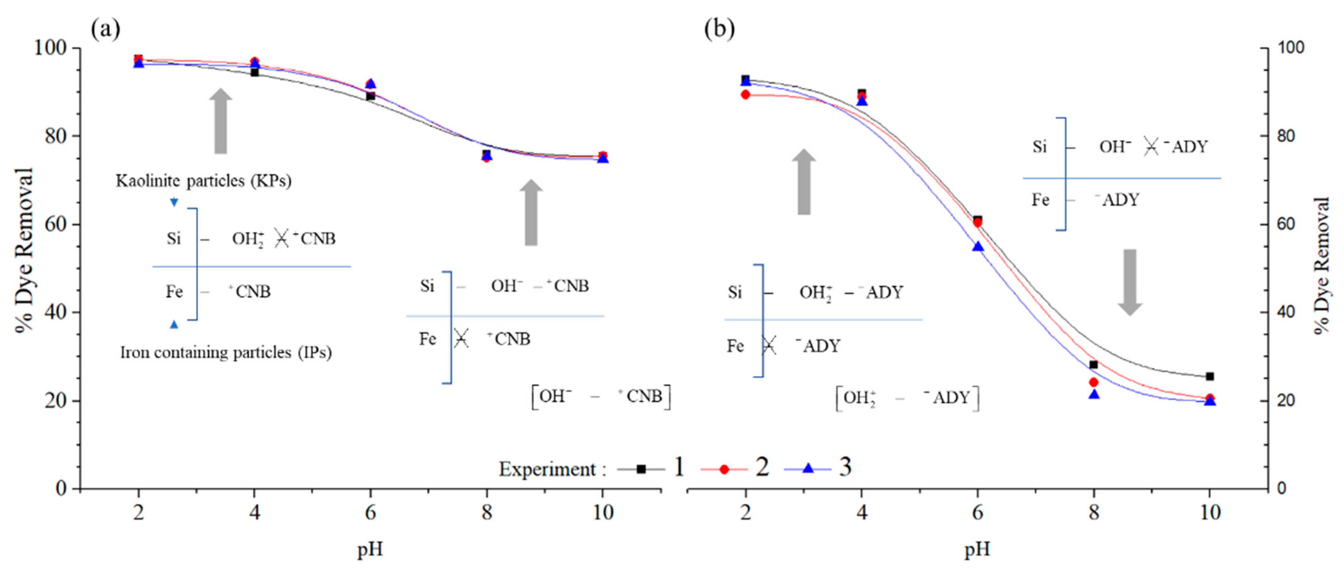
The naturally occurring clayey composite RC can efficiently remove the cationic and anionic dye, like the CNB and ADY, from water. The outcomes suggest a clayey composite constituted by IPs, KPs, and LPs. The heterogeneous composition of naturally occurring clayey composite favors different adsorption mechanisms. It opens an avenue for the separation process’s engineering. The IPs showed a strong affinity for CNB dye and the KPs and LPs for ADY dye.

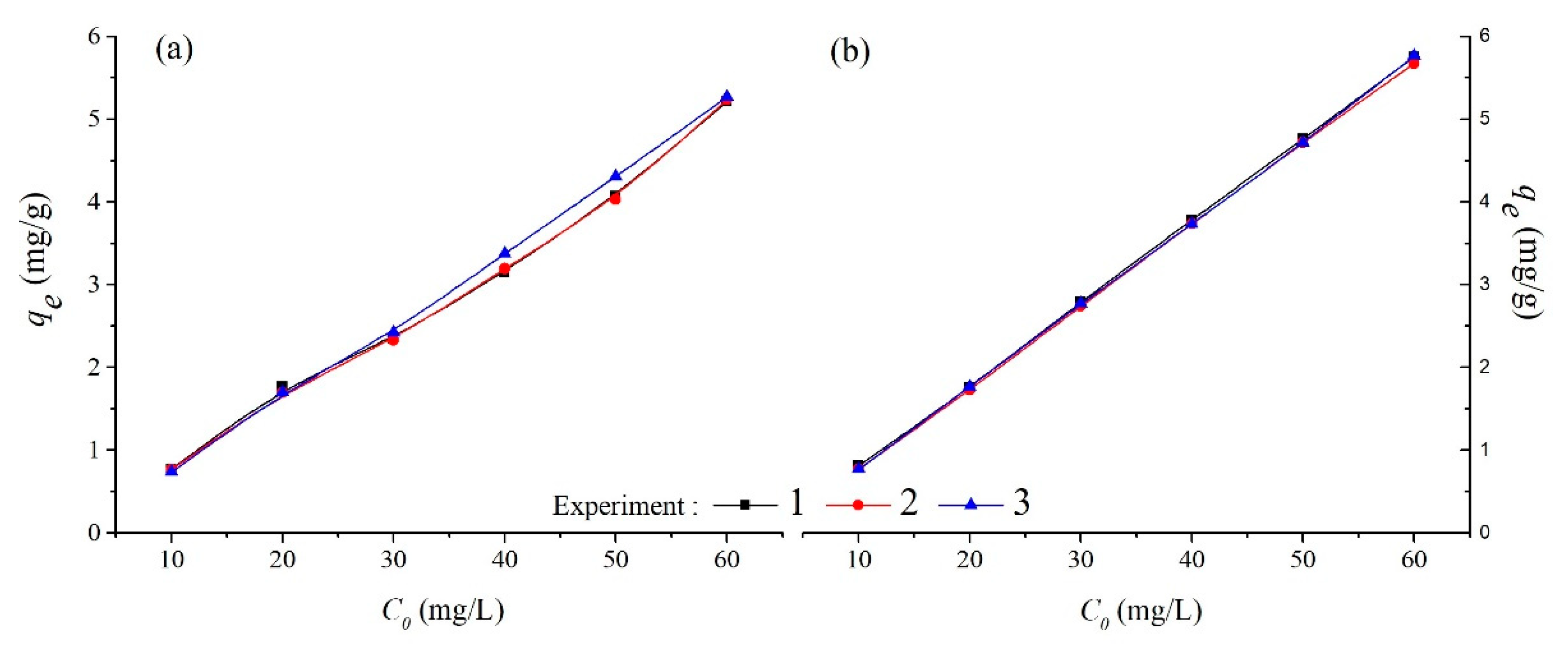
The proposed framework for studying the dye concentration effect on the adsorption capacity leads to the adsorbent dose for complete adsorption. At a pH of less than 4, the CNB and ADY removal percentage was 97% and 96%, respectively. At a pH greater than 8, the CNB and ADY removal was 75% and 25%, respectively. The study of the pH effect on dye removal allowed us to postulate the RC particles’ CNB and ADY adsorption mechanisms. The CNB adsorption happened by chemisorption of a monolayer on IPs. In contrast, the ADY adsorption occurs by the physisorption of a monolayer on KPs.

The Langmuir isotherm model fits very well with CNB experimental data. The Temkin model shows the best fit between the isotherm function and the ADY dye-adsorption data. The PSOM fits the CNB and ADY dye adsorption kinetic data on RC particles. The interparticle diffusion is not the limiting step in the CNB and ADY adsorption on RC particles at a concentration lower than 75 mg/g.