
Protection Strategy for Edge-Weighted Graphs in Disease Spread


Abstract
:1. Introduction
2. Basic Definitions
2.1. Graphs
2.2. DIL-W Ranking
3. Strategy Protection
4. Simulation of Disease Spread with Protection and Analysis Results
4.1. Data and Methodology
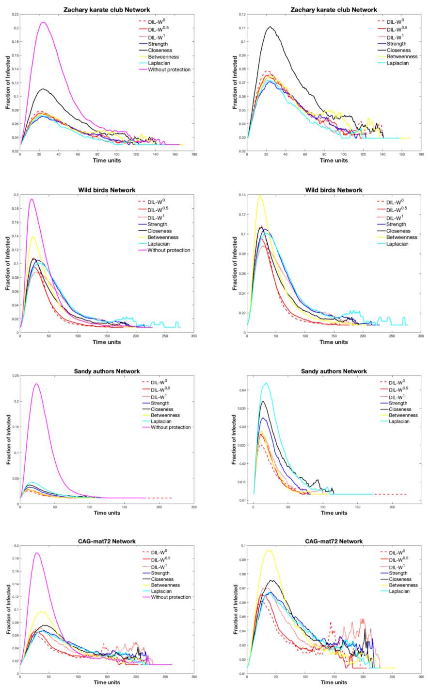
4.2. Simulation of Disease
- The probability () that a susceptible vertex is infected by one of its neighbors is given bywhere is a purely biological factor and representative of the disease and is the weight of the edge . Notice that the expression (4) can be deduced from the infection model called q-influence, assuming . (see [45,46]).
- The probability () that an infected vertex at time t will recover is given bywhere is the recovery rate.
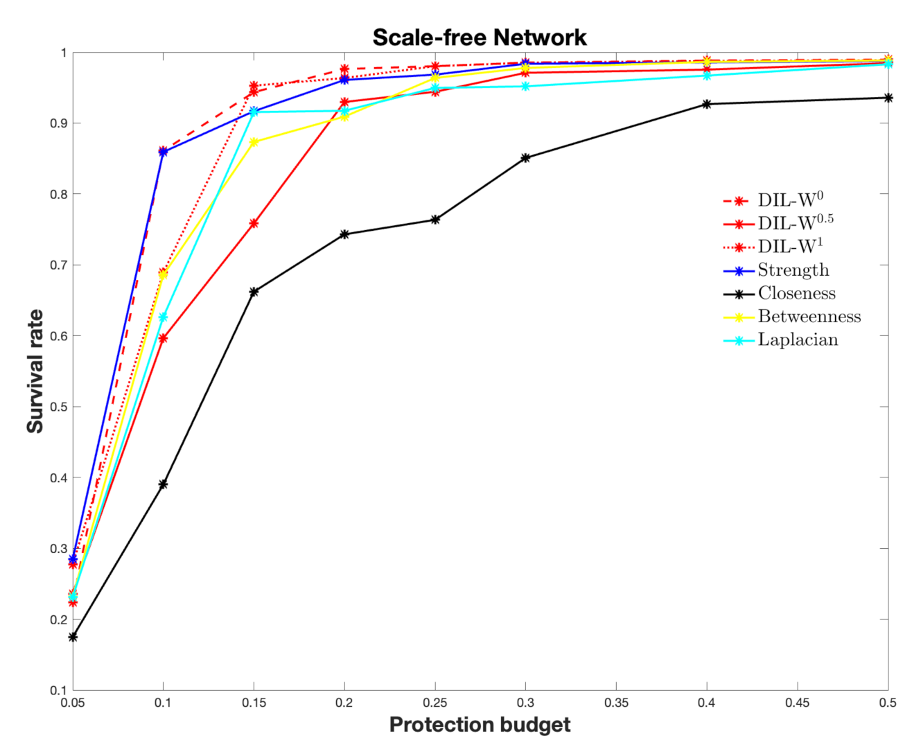
4.3. Survival Rate
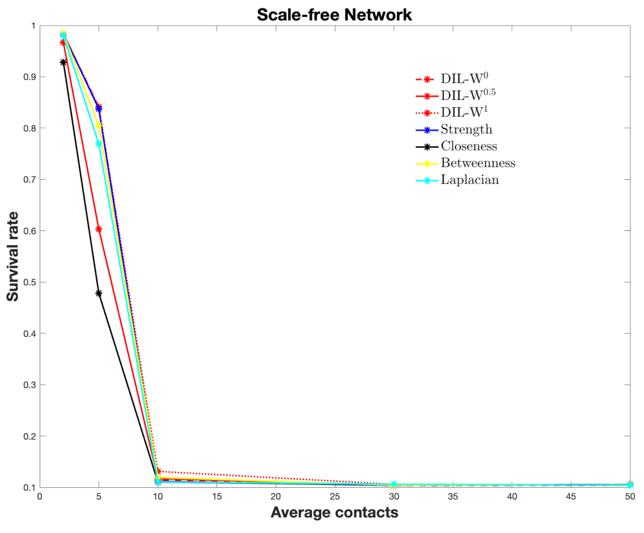
4.4. Scale-Free Network
5. Conclusions
Author Contributions
Funding
Institutional Review Board Statement
Informed Consent Statement
Data Availability Statement
Conflicts of Interest
Appendix A

| Zachary Karate Club Network | |||||||
|---|---|---|---|---|---|---|---|
| DIL-W | DIL-W | DIL-W | Strength | Closeness | Betweenness | Laplacian | |
| 5% | 0.8391 | 0.8434 | 0.8354 | 0.8406 | 0.8028 | 0.8016 | 0.8353 |
| 10% | 0.8945 | 0.8912 | 0.8941 | 0.9050 | 0.8210 | 0.8889 | 0.9015 |
| 15% | 0.9392 | 0.9367 | 0.9359 | 0.9437 | 0.8989 | 0.9333 | 0.9437 |
| 20% | 0.9510 | 0.9525 | 0.9558 | 0.9568 | 0.9276 | 0.9497 | 0.9551 |
| 25% | 0.9543 | 0.9579 | 0.9577 | 0.9593 | 0.9548 | 0.9518 | 0.9567 |
| 30% | 0.9578 | 0.9585 | 0.9572 | 0.9589 | 0.9580 | 0.9540 | 0.9597 |
| 40% | 0.9591 | 0.9603 | 0.9659 | 0.9677 | 0.9593 | 0.9681 | 0.9606 |
| 50% | 0.9657 | 0.9655 | 0.9667 | 0.9695 | 0.9603 | 0.9705 | 0.9662 |
| Wild Birds Network | |||||||
|---|---|---|---|---|---|---|---|
| DIL-W | DIL-W | DIL-W | Strength | Closeness | Betweenness | Laplacian | |
| 5% | 0.7355 | 0.7394 | 0.6447 | 0.6188 | 0.6696 | 0.6411 | 0.6212 |
| 10% | 0.7871 | 0.7942 | 0.7375 | 0.7040 | 0.7326 | 0.6952 | 0.7022 |
| 15% | 0.8721 | 0.8863 | 0.8760 | 0.8625 | 0.8149 | 0.7966 | 0.8654 |
| 20% | 0.9011 | 0.9059 | 0.9076 | 0.8943 | 0.8486 | 0.8399 | 0.8980 |
| 25% | 0.9135 | 0.9155 | 0.9208 | 0.9130 | 0.8826 | 0.8676 | 0.9078 |
| 30% | 0.9150 | 0.9226 | 0.9261 | 0.9303 | 0.8980 | 0.8941 | 0.9114 |
| 40% | 0.9361 | 0.9327 | 0.9481 | 0.9540 | 0.9018 | 0.9457 | 0.9272 |
| 50% | 0.9500 | 0.9626 | 0.9710 | 0.9762 | 0.9046 | 0.9766 | 0.9462 |
| Sandy Authors Network | |||||||
|---|---|---|---|---|---|---|---|
| DIL-W | DIL-W | DIL-W | Strength | Closeness | Betweenness | Laplacian | |
| 5% | 0.9301 | 0.9292 | 0.9296 | 0.8395 | 0.8817 | 0.9312 | 0.8329 |
| 10% | 0.9671 | 0.9637 | 0.9613 | 0.9535 | 0.9434 | 0.9615 | 0.9382 |
| 15% | 0.9738 | 0.9727 | 0.9692 | 0.9706 | 0.9513 | 0.9686 | 0.9616 |
| 20% | 0.9749 | 0.9799 | 0.9760 | 0.9779 | 0.9558 | 0.9764 | 0.9645 |
| 25% | 0.9771 | 0.9819 | 0.9822 | 0.9798 | 0.9568 | 0.9808 | 0.9773 |
| 30% | 0.9795 | 0.9837 | 0.9832 | 0.9827 | 0.9700 | 0.9829 | 0.9791 |
| 40% | 0.9824 | 0.9852 | 0.9848 | 0.9839 | 0.9680 | 0.9853 | 0.9824 |
| 50% | 0.9825 | 0.9870 | 0.9860 | 0.9860 | 0.9670 | 0.9860 | 0.9837 |
| CAG-mat72 Network | |||||||
|---|---|---|---|---|---|---|---|
| DIL-W | DIL-W | DIL-W | Strength | Closeness | Betweenness | Laplacian | |
| 5% | 0.7214 | 0.7641 | 0.7632 | 0.7734 | 0.7714 | 0.7256 | 0.7779 |
| 10% | 0.8947 | 0.8886 | 0.8792 | 0.8685 | 0.8451 | 0.8077 | 0.8706 |
| 15% | 0.9185 | 0.9308 | 0.9330 | 0.9230 | 0.8993 | 0.9085 | 0.9090 |
| 20% | 0.9323 | 0.9452 | 0.9458 | 0.9446 | 0.9285 | 0.9094 | 0.9302 |
| 25% | 0.9464 | 0.9562 | 0.9581 | 0.9588 | 0.9444 | 0.9131 | 0.9351 |
| 30% | 0.9578 | 0.9657 | 0.9672 | 0.9631 | 0.9646 | 0.9312 | 0.9426 |
| 40% | 0.9710 | 0.9745 | 0.9750 | 0.9719 | 0.9720 | 0.9456 | 0.9679 |
| 50% | 0.9770 | 0.9809 | 0.9807 | 0.9779 | 0.9781 | 0.9458 | 0.9758 |
| Scale-Free Network | |||||||
|---|---|---|---|---|---|---|---|
| DIL-W | DIL-W | DIL-W | Strength | Closeness | Betweenness | Laplacian | |
| 5% | 0.2235 | 0.2359 | 0.2773 | 0.2845 | 0.1748 | 0.2320 | 0.2312 |
| 10% | 0.8610 | 0.5965 | 0.6893 | 0.8593 | 0.3901 | 0.6857 | 0.6264 |
| 15% | 0.9437 | 0.7585 | 0.9528 | 0.9168 | 0.6622 | 0.8734 | 0.9155 |
| 20% | 0.9763 | 0.9298 | 0.9636 | 0.9609 | 0.7431 | 0.9092 | 0.9174 |
| 25% | 0.9804 | 0.9442 | 0.9803 | 0.9684 | 0.7635 | 0.9637 | 0.9497 |
| 30% | 0.9853 | 0.9710 | 0.9852 | 0.9837 | 0.8509 | 0.9778 | 0.9519 |
| 40% | 0.9882 | 0.9755 | 0.9875 | 0.9857 | 0.9268 | 0.9863 | 0.9671 |
| 50% | 0.9897 | 0.9845 | 0.9887 | 0.9875 | 0.9359 | 0.9884 | 0.9830 |
| Scale-Free Network | |||||||
|---|---|---|---|---|---|---|---|
| DIL-W | DIL-W | DIL-W | Strength | Closeness | Betweenness | Laplacian | |
| 2 | 0.9841 | 0.9667 | 0.9842 | 0.9838 | 0.9284 | 0.9847 | 0.9800 |
| 5 | 0.8411 | 0.6032 | 0.8410 | 0.8373 | 0.4783 | 0.8046 | 0.7692 |
| 10 | 0.1143 | 0.1170 | 0.1311 | 0.1118 | 0.1104 | 0.1193 | 0.1107 |
| 30 | 0.1032 | 0.1043 | 0.1059 | 0.1037 | 0.1046 | 0.1041 | 0.1061 |
| 50 | 0.1041 | 0.1045 | 0.1046 | 0.1050 | 0.1053 | 0.1048 | 0.1043 |
References
- Almasi, S.; Hu, T. Measuring the importance of vertices in the weighted human disease network. PLoS ONE 2019, 14, e0205936. [Google Scholar] [CrossRef] [Green Version]
- An, X.L.; Zhang, L.; Li, Y.Z.; Zhang, J.G. Synchronization analysis of complex networks with multi-weights and its application in public traffic network. Phys. A Stat. Mech. Appl. 2014, 412, 149–156. [Google Scholar] [CrossRef]
- Crossley, N.; Mechelli, A.; Vértes, P.; Winton-Brown, T.; Patel, A.; Ginestet, C.; McGuire, P.; Bullmore, E. Cognitive relevance of the community structure of the human brain functional coactivation network. Proc. Natl. Acad. Sci. USA 2013, 110, 11583–11588. [Google Scholar] [CrossRef] [Green Version]
- Wang, G.; Cao, Y.; Bao, Z.Y.; Han, Z.X. A novel local-world evolving network model for power grid. Acta Phys. Sin. 2009, 6, 58. [Google Scholar]
- Demongeot, J.; Ghassani, M.; Rachdi, M.; Ouassou, I.; Taramasco, C. Archimedean copula and contagion modeling in epidemiology. Netw. Heterog. Media 2013, 8, 149. [Google Scholar] [CrossRef]
- Montenegro, E.; Cabrera, E.; González, J.; Manríquez, R. Linear representation of a graph. Bol. Da Soc. Parana. De Matemática 2019, 37, 97–102. [Google Scholar] [CrossRef] [Green Version]
- Pastor-Satorras, R.; Vespignani, A. Epidemic Spreading in Scale-Free Networks. Phys. Rev. Lett. 2001, 86, 3200–3203. [Google Scholar] [CrossRef] [PubMed] [Green Version]
- Guess, A.; Nagler, J.; Tucker, J. Less than you think: Prevalence and predictors of fake news dissemination on Facebook. Sci. Adv. 2019, 5, eaau4586. [Google Scholar] [CrossRef] [Green Version]
- Yang, X.; Yang, L. Towards the epidemiological modeling of computer viruses. Discret. Dyn. Nat. Soc. 2012, 2012, 259671. [Google Scholar] [CrossRef]
- Manríquez, R.; Guerrero-Nancuante, C.; Martínez, F.; Taramasco, C. Spread of Epidemic Disease on Edge-Weighted Graphs from a Database: A Case Study of COVID-19. Int. J. Environ. Res. Public Health 2021, 18. [Google Scholar] [CrossRef] [PubMed]
- Pastor-Satorras, R.; Vespignani, A. Immunization of complex networks. Phys. Rev. E 2002, 65, 036104. [Google Scholar] [CrossRef] [Green Version]
- Cohen, R.; Havlin, S.; Ben-Avraham, D. Efficient immunization strategies for computer networks and populations. Phys. Rev. Lett. 2003, 91, 247901. [Google Scholar] [CrossRef] [Green Version]
- Tong, H.; Prakash, B.A.; Tsourakakis, C.; Eliassi-Rad, T.; Faloutsos, C.; Chau, D. On the Vulnerability of Large Graphs. In Proceedings of the 2010 IEEE International Conference on Data Mining, Sydney, NSW, Australia, 13–17 December 2010; pp. 1091–1096. [Google Scholar] [CrossRef]
- Chen, C.; Tong, H.; Prakash, B.A.; Tsourakakis, C.E.; Eliassi-Rad, T.; Faloutsos, C.; Chau, D. Node immunization on large graphs: Theory and algorithms. IEEE Trans. Knowl. Data Eng. 2015, 28, 113–126. [Google Scholar] [CrossRef] [Green Version]
- Hébert-Dufresne, L.; Allard, A.; Young, J.G.; Dubé, L.J. Global efficiency of local immunization on complex networks. Sci. Rep. 2013, 3, 1–8. [Google Scholar] [CrossRef] [Green Version]
- Zhang, Y.; Prakash, B.A. Dava: Distributing vaccines over networks under prior information. In Proceedings of the 2014 SIAM International Conference on Data Mining, Philadelphia, PA, USA, 24–26 April 2014; pp. 46–54. [Google Scholar]
- Zhang, Y.; Prakash, B.A. Data-aware vaccine allocation over large networks. ACM Trans. Knowl. Discov. Data (TKDD) 2015, 10, 1–32. [Google Scholar] [CrossRef]
- Song, C.; Hsu, W.; Lee, M. Node immunization over infectious period. In Proceedings of the 24th ACM International on Conference on Information and Knowledge Management, Melbourne, Australia, 19–23 October 2015; pp. 831–840. [Google Scholar]
- Gupta, N.; Singh, A.; Cherifi, H. Community-based immunization strategies for epidemic control. In Proceedings of the IEEE 2015 7th international conference on communication systems and networks (COMSNETS), Bangalore, India, 6–10 January 2015; pp. 1–6. [Google Scholar]
- Wang, B.; Chen, G.; Fu, L.; Song, L.; Wang, X. Drimux: Dynamic rumor influence minimization with user experience in social networks. IEEE Trans. Knowl. Data Eng. 2017, 29, 2168–2181. [Google Scholar] [CrossRef]
- Wijayanto, A.W.; Murata, T. Flow-aware vertex protection strategy on large social networks. In Proceedings of the 2017 IEEE/ACM International Conference on Advances in Social Networks Analysis and Mining (ASONAM), Sydney, NSW, Australia, 31 July–3 August 2017; pp. 58–63. [Google Scholar]
- Saxena, C.; Doja, M.; Ahmad, T. Group based centrality for immunization of complex networks. Phys. A Stat. Mech. Appl. 2018, 508, 35–47. [Google Scholar] [CrossRef] [Green Version]
- Ghalmane, Z.; El Hassouni, M.; Cherifi, H. Immunization of networks with non-overlapping community structure. Soc. Netw. Anal. Min. 2019, 9, 1–22. [Google Scholar] [CrossRef] [Green Version]
- Ghalmane, Z.; Cherifi, C.; Cherifi, H.; El Hassouni, M. Centrality in complex networks with overlapping community structure. Sci. Rep. 2019, 9, 1–29. [Google Scholar] [CrossRef] [Green Version]
- Wijayanto, A.W.; Murata, T. Effective and scalable methods for graph protection strategies against epidemics on dynamic networks. Appl. Netw. Sci. 2019, 4, 1–31. [Google Scholar] [CrossRef] [Green Version]
- Tang, P.; Song, C.; Ding, W.; Ma, J.; Dong, J.; Huang, L. Research on the node importance of a weighted network based on the k-order propagation number algorithm. Entropy 2020, 22, 364. [Google Scholar] [CrossRef] [Green Version]
- Manríquez, R.; Guerrero-Nancuante, C.; Martínez, F.; Taramasco, C. A Generalization of the Importance of Vertices for an Undirected Weighted Graph. Symmetry 2021, 13, 902. [Google Scholar] [CrossRef]
- Ren, Z.; Shao, F.; Liu, J.; Guo, Q.; Wang, B.H. Node importance measurement based on the degree and clustering coefficient information. Acta Phys. Sin. 2013, 62, 128901. [Google Scholar]
- Musiał, K.; Juszczyszyn, K. Properties of bridge nodes in social networks. In International Conference on Computational Collective Intelligence; Springer: Berlin/Heidelberg, Germany, 2009; pp. 357–364. [Google Scholar]
- Liu, J.; Xiong, Q.; Shi, W.; Shi, X.; Wang, K. Evaluating the importance of nodes in complex networks. Phys. A Stat. Mech. Appl. 2016, 452, 209–219. [Google Scholar] [CrossRef] [Green Version]
- Chartrand, G.; Lesniak, L. Graphs and Digraphs, 1st ed.; Springer: Berlin/Heidelberg, Germany, 1996. [Google Scholar]
- West, D.B. Introduction to Graph Theory, 2nd ed.; Prentice Hall: Upper Saddle River, NJ, USA, 2001. [Google Scholar]
- Opsahl, T.; Agneessens, F.; Skvoretz, J. Node centrality in weighted networks: Generalizing degree and shortest paths. Soc. Netw. 2010, 32, 245–251. [Google Scholar] [CrossRef]
- Vinterbo, S.A. Privacy: A machine learning view. IEEE Trans. Knowl. Data Eng. 2004, 16, 939–948. [Google Scholar] [CrossRef]
- Latora, V.; Marchiori, M. Efficient Behavior of Small-World Networks. Phys. Rev. Lett. 2001, 87, 198701. [Google Scholar] [CrossRef] [Green Version]
- Lai, Y.; Motter, A.; Nishikawa, T. Attacks and cascades in complex networks. In Complex Networks; Springer: Berlin/Heidelberg, Germany, 2004; pp. 299–310. [Google Scholar]
- Zachary, W.W. An Information Flow Model for Conflict and Fission in Small Groups. J. Anthropol. Res. 1977, 33, 452–473. [Google Scholar] [CrossRef] [Green Version]
- Firth, J.A.; Sheldon, B.C. Experimental manipulation of avian social structure reveals segregation is carried over across contexts. Proc. R. Soc. B Biol. Sci. 2015, 282, 20142350. [Google Scholar] [CrossRef] [Green Version]
- Imrich, W.; Klavzar, S. Product Graphs: Structure and Recognition; Wiley: Hoboken, NJ, USA, 2000. [Google Scholar]
- Barrat, A.; Barthelemy, M.; Pastor-Satorras, R.; Vespignani, A. The architecture of complex weighted networks. Proc. Natl. Acad. Sci. USA 2004, 101, 3747–3752. [Google Scholar] [CrossRef] [Green Version]
- Brandes, U. A faster algorithm for betweenness centrality. J. Math. Sociol. 2001, 25, 163–177. [Google Scholar] [CrossRef]
- Newman, M. Scientific collaboration networks. II. Shortest paths, weighted networks, and centrality. Phys. Rev. E 2001, 64, 016132. [Google Scholar] [CrossRef] [Green Version]
- Qi, X.; Fuller, E.; Wu, Q.; Wu, Y.; Zhang, C.Q. Laplacian centrality: A new centrality measure for weighted networks. Inf. Sci. 2012, 194, 240–253. [Google Scholar] [CrossRef]
- Rossi, R.; Ahmed, N.K. The Network Data Repository with Interactive Graph Analytics and Visualization. In Proceedings of the Twenty-Ninth AAAI Conference on Artificial Intelligence, Austin, TX, USA, 25–30 January 2015. [Google Scholar]
- Zhang, Z.; Wang, H.; Wang, C.; Fang, H. Modeling epidemics spreading on social contact networks. IEEE Trans. Emerg. Top. Comput. 2015, 3, 410–419. [Google Scholar] [CrossRef] [Green Version]
- Pastor-Satorras, R.; Castellano, C.; Van Mieghem, P.; Vespignani, A. Epidemic processes in complex networks. Phys. Rev. Lett. 2015, 87, 925–980. [Google Scholar]
- Liu, J.; Zhang, T. Epidemic spreading of an SEIRS model in scale-free networks. Commun. Nonlinear Sci. Numer. Simul. 2011, 16, 3375–3384. [Google Scholar] [CrossRef]
- Liu, M.-X.; Jiong, R. Modelling the spread of sexually transmitted diseases on scale-free networks. Chin. Phys. B 2009, 1, 2115–2120. [Google Scholar]
- Song, W.; Zang, P.; Ding, Z.; Fang, X.; Zhu, L.; Zhu, Y.; Bao, C.; Chen, F.; Wu, M.; Peng, Z. Massive migration promotes the early spread of COVID-19 in China: A study based on a scale-free network. Infect. Dis. Poverty 2020, 9, 1–8. [Google Scholar] [CrossRef]
- Schneeberger, A.; Mercer, C.; Gregson, S.; Ferguson, N.; Nyamukapa, C.; Anderson, R.; Johnson, A.; Garnett, G. Scale-free networks and sexually transmitted diseases: A description of observed patterns of sexual contacts in Britain and Zimbabwe. Sex. Transm. Dis. 2004, 31, 380–387. [Google Scholar] [CrossRef]
- Moreno, Y.; Vazquez, A. Disease spreading in structured scale-free networks. Eur. Phys. J. B-Condens. Matter Complex Syst. 2003, 31, 265–271. [Google Scholar] [CrossRef] [Green Version]
- Yang, P.; Wang, Y. Dynamics for an SEIRS epidemic model with time delay on a scale-free network. Phys. A Stat. Mech. Appl. 2019, 527, 121290. [Google Scholar] [CrossRef]
- Ke, H.; Yi, T. Immunization for scale-free networks by random walker. Chin. Phys. 2006, 15, 2782. [Google Scholar] [CrossRef]
- Barabási, A.; Albert, R. Emergence of Scaling in Random Networks. Science 1999, 286, 509–512. [Google Scholar] [CrossRef] [Green Version]


| Zachary Karate Club | Wild Bird | Sandy Authors | CAG-mat72 | |
|---|---|---|---|---|
| Zachary | Wild Birds | Sandy Authors | CAG-mat72 | |
|---|---|---|---|---|
| DIL-W | 0.8946 | 0.7871 | 0.9671 | 0.8947 |
| DIL-W | 0.8912 | 0.7943 | 0.9637 | 0.8887 |
| DIL-W | 0.8941 | 0.7375 | 0.9613 | 0.8792 |
| Strength | 0.9051 | 0.7041 | 0.9536 | 0.8685 |
| Closeness | 0.8211 | 0.7327 | 0.9435 | 0.8451 |
| Betweenness | 0.8890 | 0.6952 | 0.9616 | 0.8078 |
| Laplacian | 0.9016 | 0.7023 | 0.9382 | 0.8707 |
Publisher’s Note: MDPI stays neutral with regard to jurisdictional claims in published maps and institutional affiliations. |
© 2021 by the authors. Licensee MDPI, Basel, Switzerland. This article is an open access article distributed under the terms and conditions of the Creative Commons Attribution (CC BY) license (https://creativecommons.org/licenses/by/4.0/).
Share and Cite
Manríquez, R.; Guerrero-Nancuante, C.; Taramasco, C. Protection Strategy for Edge-Weighted Graphs in Disease Spread. Appl. Sci. 2021, 11, 5115. https://doi.org/10.3390/app11115115
Manríquez R, Guerrero-Nancuante C, Taramasco C. Protection Strategy for Edge-Weighted Graphs in Disease Spread. Applied Sciences. 2021; 11(11):5115. https://doi.org/10.3390/app11115115
Chicago/Turabian StyleManríquez, Ronald, Camilo Guerrero-Nancuante, and Carla Taramasco. 2021. "Protection Strategy for Edge-Weighted Graphs in Disease Spread" Applied Sciences 11, no. 11: 5115. https://doi.org/10.3390/app11115115
APA StyleManríquez, R., Guerrero-Nancuante, C., & Taramasco, C. (2021). Protection Strategy for Edge-Weighted Graphs in Disease Spread. Applied Sciences, 11(11), 5115. https://doi.org/10.3390/app11115115