Article

A Dispatching-Fuzzy AHP-TOPSIS Model for Scheduling Flexible Job-Shop Systems in Industry 4.0 Context

by
Miguel Ortíz-Barrios
1,
Antonella Petrillo
2,
Fabio De Felice
3,*,
Natalia Jaramillo-Rueda
1,
Genett Jiménez-Delgado
4 and
Luz Borrero-López
1
1
Department of Industrial Management, Agroindustry and Operations, Universidad de la Costa CUC, Barranquilla 080003, Colombia
2
Department of Engineering, University of Napoli “Parthenope”, 80143 Naples, Italy
3
Department of Civil and Mechanical Engineering, University of Cassino and Southern Lazio, 03043 Cassino, Italy
4
Department of Industrial Engineering, Institución Universitaria ITSA, Barranquilla 080003, Colombia
*
Author to whom correspondence should be addressed.
Appl. Sci. 2021, 11(11), 5107; https://doi.org/10.3390/app11115107
Submission received: 3 May 2021 / Revised: 23 May 2021 / Accepted: 27 May 2021 / Published: 31 May 2021

Abstract

:
Scheduling flexible job-shop systems (FJSS) has become a major challenge for different smart factories due to the high complexity involved in NP-hard problems and the constant need to satisfy customers in real time. A key aspect to be addressed in this particular aim is the adoption of a multi-criteria approach incorporating the current dynamics of smart FJSS. Thus, this paper proposes an integrated and enhanced method of a dispatching algorithm based on fuzzy AHP (FAHP) and TOPSIS. Initially, the two first steps of the dispatching algorithm (identification of eligible operations and machine selection) were implemented. The FAHP and TOPSIS methods were then integrated to underpin the multi-criteria operation selection process. In particular, FAHP was used to calculate the criteria weights under uncertainty, and TOPSIS was later applied to rank the eligible operations. As the fourth step of dispatching the algorithm, the operation with the highest priority was scheduled together with its initial and final time. A case study from the smart apparel industry was employed to validate the effectiveness of the proposed approach. The results evidenced that our approach outperformed the current company’s scheduling method by a median lateness of 3.86 days while prioritizing high-throughput products for earlier delivery.

1. Introduction

Current market trends, the variety of consumer demand, the short life cycle of the product, and competitive pressure have pushed companies to tackle the problem of reduction of production costs through better management of available resources. One fundamental tool is represented by the scheduling algorithms for the optimization of production [1]. Scheduling problems are decision-making problems in which the factor of time is of fundamental importance, understood as a (scarce) resource to be allocated in an optimal way [2]. In the context of industrial manufacturing, scheduling consists in determining the sequential allocation of jobs to the machines, which optimizes a certain objective function and respects at the same time the constraints imposed [3]. More specifically, a scheduling problem is uniquely described by three factors: architecture of the production system, process parameters, and any constraints of the function to be optimized. The scheduling problem has been analyzed in numerous studies, which have allowed the development of different models that represent it and different methods to solve it [4]. Several applications can be traced back to scheduling problems: the regulation of user access to a service, the assignment of operations at workstations during the transformation process of a product, the timing of activities to be carried out within a project complex, the assignment of classrooms to a set of classes, regulation of vehicle accesses at an intersection through traffic light control, the assignment of tracks to railway trains, and the use of tracks and/or gates by planes arriving or departing from an airport. Scheduling problems can be represented through appropriate models [5,6,7,8,9,
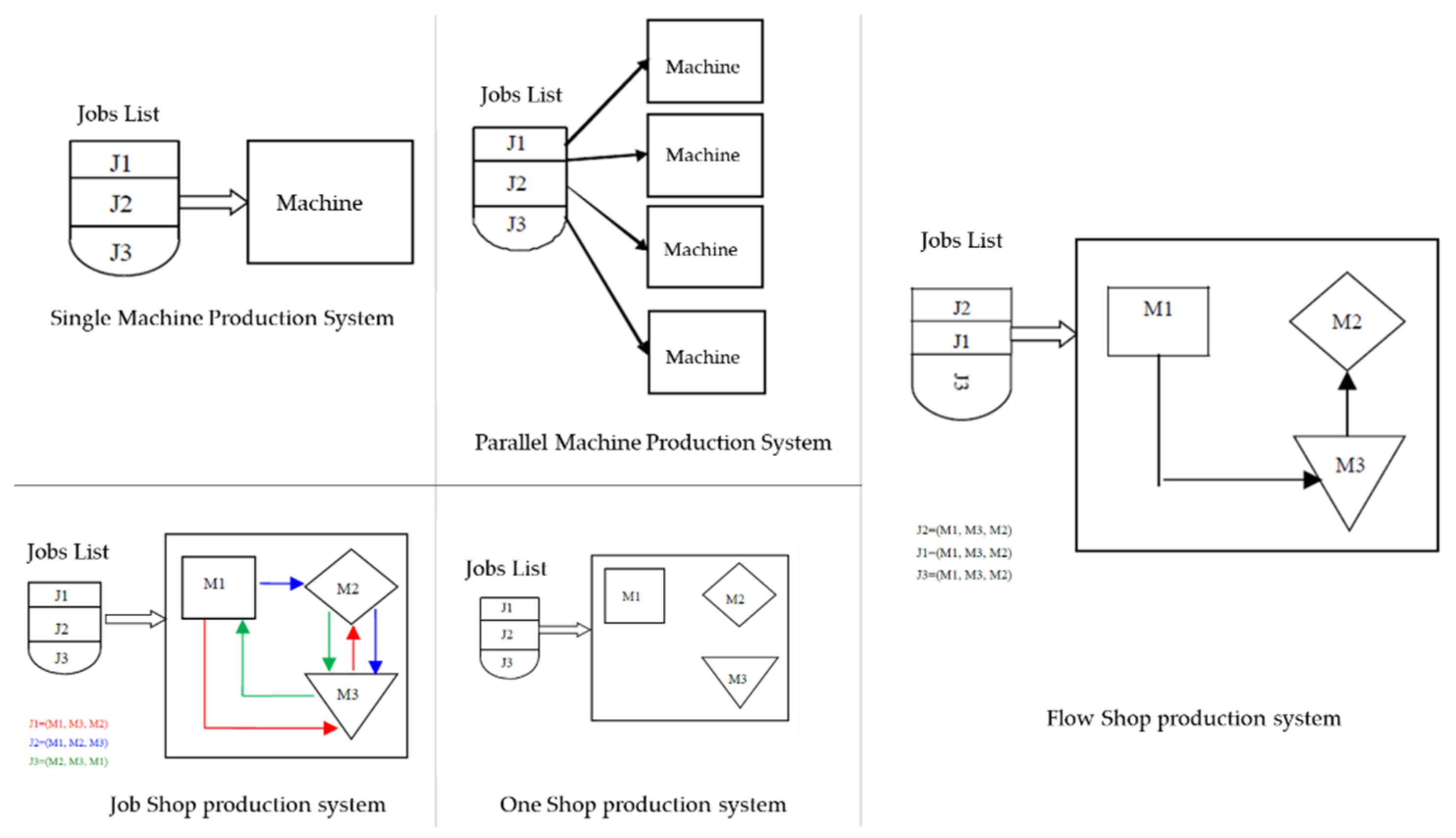
10]. The main scheduling models are (1) single machine, (2) parallel machines, (3) job shop, (4) flexible job shop, (5) flow shop, (6) flexible flow shop, and (7) open shop. The complexity of the models depends on the resources available, the type of constraints present, and the choice of objectives. In Figure 1, the main models used for the scheduling problems are illustrated.
An extension of the classical job shop scheduling problem is the flexible job-shop system (FJSS). It is a very important topic in the field of production management and smart manufacturing [11]. FJSS algorithms should be adapted to effectively support the response of available operational technology (OT) within the day-to-day operations of smart companies. However, classical scheduling methods are generally incapable of solving complex problems characterized by a continuous upgrading of the production mode of the manufacturing system [12]. A key aspect to be addressed in this aim is the adoption of a multi-criteria operation selection approach, incorporating the current dynamics of smart FJSS [13]. To face this challenge, this paper proposes a hybrid and innovative model of a dispatching algorithm based on fuzzy AHP (FAHP) and TOPSIS. In particular, FAHP was used to calculate the criteria weights under uncertainty, and TOPSIS was later applied to rank the eligible operations. A case study from the smart apparel industry was employed to validate the effectiveness of the proposed approach. In this case, a FJSS with two objectives (minimize the average lateness and maximize throughput), seven sub-processes, 13 products, and 29 orders was considered. The results evidenced that our approach outperformed the current company’s scheduling method by a median lateness of 3.86 days while prioritizing high-throughput products for earlier delivery. Our approach differs from previous work published in the literature that tended to focus solely on the classical approach. Our aim is to propose an integrated approach for the flexible job-shop scheduling problem for smart manufacturing that combines the benefits of each method.
The rest of the paper is structured as follows: Section 2 presents a literature review on FJSS and smart manufacturing. The aim of Section 2 is to briefly outline the trends in the topic analyzed. Section 3 explains materials and methods. Thereafter, Section 4 presents an illustrative example from the smart apparel industry. Results and discussion of the main findings of the research are analyzed in Section 5. Finally, Section 6 provides implications for research and future development.

2. Literature Review on FJSS and Smart Manufacturing

The topic of scheduling flexible job-shop systems (FJSS) is a theme analyzed in the scientific literature as early as the 1980s, as demonstrated by a survey carried out on Elsevier’s Scopus, the largest abstract and citation database of peer-reviewed literature. In order to identify publications on FJSS, an investigation using the string “Scheduling flexible job-shop systems” has been used. Only articles in which the string was found in the (1) article title, (2) abstract, or (3) keywords were analyzed (TITLE-ABS-KEY (scheduling AND flexible AND job-shop AND systems). The analysis on Scopus found 961 documents resulting from 1980 to 2021 (May 2021, period of investigation). The research highlighted a growth in the number of publications. Most of them have been published in 2020 (86 documents). Figure 2 shows the trend of publications over the years.
The investigation on Scopus highlighted that the three most productive countries are China (287; 30%), the United States (123; 13%), and France (67; 7%). The result is not a surprise, because it only confirms that “big” countries in terms of population are obviously the most productive ones. Interestingly, other countries like Japan are also making great advances now in plant scheduling. A worthy study was proposed in 2019 by Sun et al. [14] in which a hybrid cooperative coevolution algorithm (hCEA) for the minimization of fuzzy makespan was proposed. Furthermore, in 2015, Gen et al. [15] developed hybrid genetic algorithms (HGA) and multiobjective HGA (Mo-HGA) to solve manufacturing scheduling problems.
We have also investigated other parameters, as explained below. In particular, the analysis of documents by type pointed out the following distribution: articles (548; 57%), conference papers (346; 36%), conference reviews (44; 5%), books and chapters (8; 1%), reviews (8; 1%), and other (Letter. Editorial. Note 5; 1%). The analysis of documents by subject area highlighted that most of the publications (92%) belong to the following area: engineering (34%); computer science (29%); mathematics (10%); decision sciences (10%); business, management, and accounting (8%); and other (9%).
The literature on the subject is certainly very extensive. Thus, we investigated a very precise aspect related to smart manufacturing. In the context of “smart manufacturing”, we have selected 19 documents in line with our research goal. We selected the documents by examining the keywords and the field of application by analyzing all the documents resulting from the investigation. 
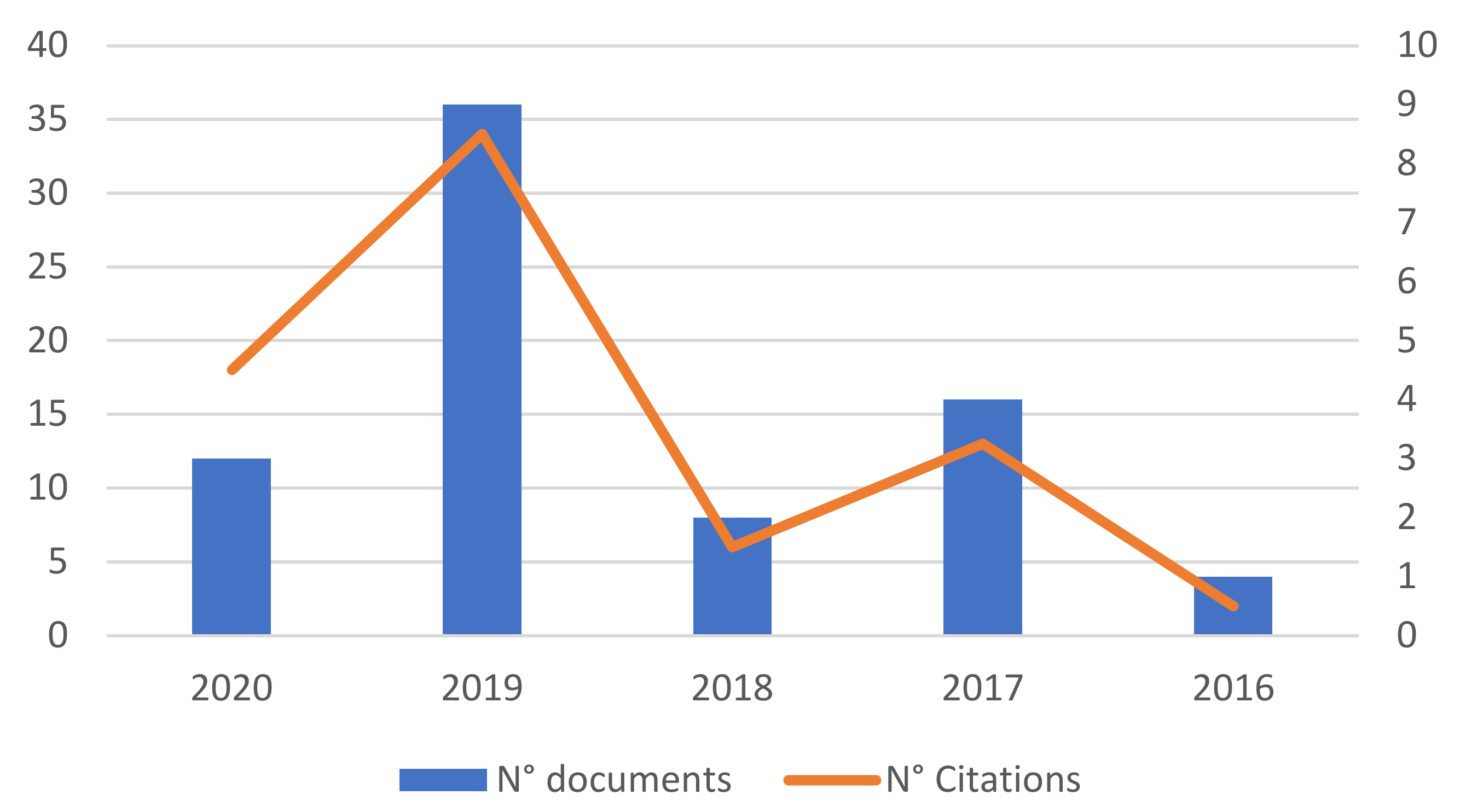
Table 1 summarizes the number of documents by year and by type.
Figure 3 depicts the time distribution of the papers and the number of citations.
According to the literature analysis, we have analyzed in detail the 19 documents as shown below. In particular, the following considerations emerged.
Recently, Li et al. [16] developed an optimization algorithm to solve the FJSP in the context of a smart production plant. Ghaleb et al. [17] proposed a real-time scheduling model for the FJSP. Mihoubi et al. [18] proposed a genetic algorithm to solve the FJSP problem. In 2019, Lim et al. [19] proposed a reusable scheduling problem decomposition framework for Industry 4.0 that facilitates agent-embedded optimization. In 2019, Vazan et al. [20] defined a simulation model of the smart flexible manufacturing system with interchangeable workplaces. A different point of view was introduced by Ma et al. in 2019 [21]. They introduced an anarchic manufacturing model to evaluate the relative flexibility of a representative hierarchical system against an anarchic system in a job shop scenario. A survey on the scheduling in production in the context of Industry 4.0 systems was proposed by Dolgui et al., 2019 [22]. Heger and Voß [23] presented a scheduling and dispatching approach for a flexible job shop incorporating travel times of autonomous guided vehicles. Some studies propose functional architecture for flexible manufacturing systems [24,25]. Other studies develop a heuristics model and algorithm to optimize and support scheduling flexible job-shop systems [26,27,28,29,30]. In 2017, a heterarchical approach based on intelligent products was analyzed by Bouazza et al. [31]. Dolgui with Ivanov and Sokolov [32] developed a model of job shop scheduling in a customized manufacturing process. A simulation approach was proposed in some studies such as by Son et al. [33] that simulate a flexible manufacturing system for producing aircraft. A novel approach based on Machine to Machine (M2M) was well argued by Yuan et al. [34]. From our point of view, it was also important to analyze the keywords in common with the selected documents and the most used ones. In this regard, Table 2 shows a classification of documents by keywords.
The analysis of the literature review pointed out that the selected documents are very heterogeneous with each other. Most of them propose traditional methods for solving scheduling problems. Some of them highlight the importance of communication technologies as the key tool that enables the interconnection among a priori isolated business processes. Among them, Jacob et al. [35] analyzed the use of 5G and Tian et al. [36] investigated the use of the Internet of Things, as they enabled manufacturing enterprise information systems to solve scheduling problems. Already in 2010, Zhao et al. [37] proposed a hybrid algorithm for production scheduling integration in holonic manufacturing systems. It is also clear that in modern competitive companies, the scheduling problem is also associated with correct maintenance, as pointed out by some authors [38,39]. In addition, it is important to note that, although several studies on FJSS have been published, the integration of a decision tool based on MCDA is not treated to solve the flexible job shop scheduling problem. However, it is clear that in a dynamic and complex environment such as the modern smart factories, the use of multi-criteria decision-making methods could represent an opportunity from a practical and problem-solving point of view, as stated by several authors [40,41,42]. In this way, more perspectives can be considered. It is a fundamental management strategy from a smart manufacturing perspective in which many factors must be taken into consideration. In fact, scheduling is a “form” of decision-making, which consists in allocating finite resources in such a way that a given goal is optimized. A scheduling problem contains the following information: (1) the decision variable and (2) the criterion by which the decision variables are evaluated (performance measure). In other words, a solution to a scheduling problem consists in identifying the optimal decision in the sense specified by the particular criterion adopted. As -making methods definitely represent a very effective tool in modern factories from a managerial point of view, our research aims to cover the literature gap.

3. Materials and Methods

3.1. Problem Definition and Modeling Phase

The suggested dispatching-fuzzy AHP-TOPSIS (DFT) methodology entails the combination of three methods for solving the FJSP in smart manufacturing: the dispatching algorithm, the fuzzy analytic hierarchy process, and TOPSIS. Such a combination is developed through a four-phase methodology outlined in Figure 4. The proposed approach is an adaptation of the algorithm presented by Calleja and Pastor [43]. A more detailed explanation of each phase is provided below:
Phase 1: In this step, the production system is characterized by defining the route of each product reference, the available machines associated with each sub-process, the setup times ( S U t j ), and the processing times ( p i , k , l , j ), whereas the jobs are fully detailed in terms of their features. This information defines the N subset, which covers all the operations to be scheduled. Following this, the E subset, comprised of all operations eligible for immediate execution (the first operation of each job), is arranged while specifying their r 1 , k , l values. The f p j is then defined in each machine, and f p m i n is finally identified from the list of m machines.
Figure 4. The proposed DFT approach for solving the FJSP.
Applsci 11 05107 g004
Phase 2: In the next step, the machine with f p m i n is selected. Then, all the candidate operations associated with the selected machine are enlisted. In the case of various machines with f p m i n , the operation to be scheduled must be chosen by implementing the operation prioritization framework depicted in Phase 3. A f p m i n = α denotes that all the operations have been programmed.
Phase 3: This stage involves choosing the operation to be scheduled or enlisted in the subset P. In this regard, there are two possible scenarios. In the case of a set of eligible operations, the DFT (Dispatching-Fuzzy AHP-TOPSIS) approach must be implemented. To this end, an operation prioritization model has to be first defined considering the criteria or job features that are of special interest to the company. FAHP (see Section 3.2) is then employed to estimate the relative importance of these criteria under uncertainty. After this, TOPSIS (see Section 3.3) calculates a priority index (closeness coefficient) for each eligible operation. The operation with the highest index is finally selected to be accordingly included in the subset P. The remaining scenario is the one in which there is only one candidate operation; in such a case, the scheduler must pass it immediately to the subset P without implementing the operation prioritization model here proposed.
Phase 4: The final step of this methodology is to enlist the selected operation while outlining its start and end times. The end time is calculated by using the formula specified in Figure 3 considering whether j = j′. Following this, the f p j value of the machine j associated with the selected operation is updated. r p i , k , l ,   j and f p m i n are then computed according to Figure 3. Ultimately, the scheduler must return to Phase 1 until all the operations are scheduled ( f p m i n = α ).

3.2. Fuzzy Analytic Hierarchy Process (FAHP)

Fuzzy logic was integrated with the AHP technique to address the lack of clarity arising from human judgments, for example, in paired comparisons [44,45,46]. To this end, fuzzy sets provide a solid foundation for solving real-world MCDM problems, which inevitably involve some level of noise in their structure. Under consideration of these aspects, AHP becomes FAHP. The judgments are represented by triangular numbers M denoted by (a. b. c), and the membership function is described as follows:
μ M ~ x = x a b a . a x b c x c b . b x c   0 . o t h e r w i s e
Here, < a b c < .
The lower and upper limits are a and c, whereas the strongest degree is symbolized by the parameter b. The fuzzy triangular numbers to be employed in evaluating the importance of operation selection criteria and sub-criteria are described in Table 3. A shorter version of the Saaty’s scale (5-point scale) is proposed to accelerate the decision-making process and reduce bias when making the paired judgments [47].
The FAHP procedure is as follows:
Step 1: The fuzzy triangular numbers referred to in Table 3 are used to make a pairwise comparison between criteria and sub-criteria. In this way, it is possible to obtain the matrix of fuzzy judgments for A ˜ K (Equation (1)):
A ˜ K = a ˜ 11 k a ˜ 12 k a ˜ 1 n k a ˜ 21 k a ˜ 22 k a ˜ 2 n k a ˜ n 1 k a ˜ n 2 k a ˜ n n k
a ˜ i j k represents the k th decision-maker’s predilection of i th decision element (criterion/sub-criterion) over j th decision element (criterion/sub-criterion).
Step 2: If the decision is supported by a decision-making group, the comparisons should be aggregated by applying Equation (2). Here, K represents the number of experts involved in the judgment process. After this, the initial matrix of fuzzy comparisons is updated, as shown in Equation (3).
a ˜ i j = a ˜ i j 1 a ˜ i j 2 a ˜ i j k K
A ˜ = a 11 ˜ a ˜ n 1 a 1 n ˜ a ˜ n n
Step 3: The geometric mean of the fuzzy comparisons r ˜ i for each decision element (criterion or sub-criterion) is computed, taking Equation (4) as a reference:
  r ˜ i = j = 1 n a ˜ i j 1 / n .   i = 1.2 . . n
Step 4: The fuzzy relative priorities of all criteria ( w ˜ i ) are estimated by employing Equation (5)
w ˜ i = r ˜ i r ˜ 1 r ˜ 2 r ˜ n 1 = l w i . m w i . u w i
Step 5:  ( w ˜ i ) is defuzzified using the center of area method [48] described in Equation (6). Here, M i denotes a non-fuzzy number.
M i = l w i + m w i + u w i 3
Step 6:  M i is normalized by implementing Equation (7)
N i = M i i = 1 n M i

3.3. Technique for Order of Preference by Similarity to Ideal Solution (TOPSIS)

TOPSIS is a multi-criteria decision method developed by Hwang and Yoon [49] for ranking alternatives considering the shortest distance from the positive-ideal solution (PIS) and the farthest separation from the negative-ideal solution (NIS) [50,51]. The outcome is an indicator called “closeness coefficient” (priority index) ranging between 0 and 1, which enables schedulers, production managers, and practitioners to prioritize operations swiftly. The TOPSIS technique also holds the following advantages:
  • It can consider both conflicting quantitative and qualitative features, a context often found in scheduling scenarios where the operations need to be prioritized according to a set of selection criteria [52].
  • The FJS algorithms often utilize one prioritization rule and apply others in case of a tie among different operations or jobs; however, the closeness coefficient derived from TOPSIS can be adopted as an overall measure representing these rules simultaneously and thereby emulating the real decision-making scenario addressed by production managers and practitioners.
  • It allows decision-makers to establish how the operation/job priority may change if its features are modified during the negotiation process with a client or in presence of different market and production configuration conditions. In this regard, sensitivity analysis can be fully underpinned based on separations from PIS and NIS [53,54,55,56].
The general TOPSIS procedure is outlined in Figure 5 [57]:
Step 1: A decision matrix X   with “ m ” operations and “ n ” sub-criteria is created via Equation (8). X i j is the value of the sub-criterion S j   j = 1 ,   2 , , n   in each operation O i i = 1 ,   2 , , m .
X = O 1 O 2 O 3 O M S 1 x 11 x 21 x 31 x m 1 S 2 x 12 x 22 x 32 x m 2 S n x 1 n x 2 n x 3 n x m n
Step 2: The normalized decision matrix R   is calculated using Equation (9). n i j is the norm used by TOPSIS via Equation (10). Additionally, r i j is defined as the element of this matrix.
R = X · n i j
n i j = x i j i = 1 y x i j 2
Step 3: The weighted normalized decision matrix V is obtained using Equation (11). The sub-criteria weights ( w j ) are those resulting from the FAHP method.
V = w j r i j = v i j
Step 4: The ideal ( C + ) and anti-ideal C scenarios are established according to Equations (12) and (13), respectively:
C + = c i m a x i j | j J .   c i m i n i j   | j     J f o r   i = 1.2 .   . m c 1 + . c 2 + . . c j + . . c n +
C = c i m i n i j | j J .   c i m a x i j   | j     J f o r   i = 1.2 .   . m = c 1 . c . . c j . . c n    
Considering that:
J = j = 1.2 . . n | j   a s s o c i a t e d   w i t h   t h e   b e n e f i t   s u b c r i t e r i o n J ´ = j = 1.2 . . n | j   a s s o c i a t e d   w i t h   t h e   c o s t   s u b c r i t e r i o n
Step 5: The separation measures of each operation to C + and C are calculated using the Euclidean separation via Equations (14) and (15).
Euclidean separation from ideal scenario
d i + = j = 1 n c i j c j + 2                 i = 1.2 . . m
Euclidean separation from anti-ideal scenario
d i = j = 1 n c i j c j 2                 i = 1.2 . . m
Step 6: The relative closeness coefficient C C i is calculated by using Equation (16).
C C i = d i d i + + d i .             0 < C C i < 1 .             i = 1.2 . .   m  
Step 7: The operations are ranked according to C C i .

4. Numerical Experiment for a Smart Apparel Industry

The DFT algorithm here proposed was implemented in the production system of a South American textile firm (13/13/G/Tmed) whose demand schedule is comprised of 29 jobs. The process steps and sequence of operations are outlined in Figure 6.
Six main processes compose this system: WEAVING, DYEING, PRINTING, CUTTING, WHIPSTITCHING, and CLEANING. In particular, WEAVING has a set of three worker-machines (T1, T2, and T3), while DYEING can be performed by four machines (C1, C2, C3, and C4). On the other hand, there is only one PRINTING machine (E), supported by a manufacturing cell. In addition, two machines (CL1 and CL2) can carry out the WHIPSTITCHING sub-process. Finally, two worker cells (LP1 and LP2) are available for underpinning the CLEANING stage. In this case, the reference scheduling date is 31 January. On a different tack, as observed in Figure 5, each product type follows a specific processing route with m machines capable of performing the operations at different production rhythms and thereby configuring the FJSS. Additionally, the regular working period is 24 h per day. The arduous task then lies in scheduling a system with a variety of product references, orders, transfer times, and machines with different production speeds and setup times while minimizing the average lateness, a characteristic scenario of an NP-hard problem [58].
Table A1 (Appendix A) enlists the processing times (in min) of each sub-process in each machine j. In this table, “-“ denotes that a particular machine is not technically available for processing the reference or the sub-process is not part of the reference operation route. For instance, PRINTING is not a sub-process within the production path of SINGLE COLOR BEDCOVER and SINGLE FRINGE COLORED BEDCOVER, whereas the DYEING department does not process WHITE MULERA units. A different scenario is observed in references such as STAMPED SINGLE BEDCOVER and STAMPED DOUBLE BEDCOVER that go through all the sub-processes integrating the FJSS.
The company currently employs the earliest delivery date (EDD) approach, where the orders are processed considering the earliest due date first.
The demand schedule containing the delivery dates of these jobs is shown in Table A2. This table also reveals the presence of tardy jobs (31.03%; n = 9 jobs), whose days of tardiness are specified in the DOT column. The order quantity, average monthly demand (MD) throughput, and % of tardiness are also outlined in this table. Table A2 (Appendix A) presents the customer type and quantity related to the orders integrating the demand schedule. This information is useful for the deployment of the DFT approach (operation selection policy) proposed in this paper. The significant proportion of tardy jobs, the great percentage of tardiness in some high-priority references, and the need for reducing lateness as a competitive strategy have motivated the company schedulers to implement the proposed framework. If not addressed, these inefficiencies may result in possible financial sanctions and loss of customer loyalty to the firm.
On a different note, Table A3 (Appendix A) depicts the setup times and available machines for each operation. In this case, the setup times include all the activities related to the machine preparation and work-in-process (WIP) mounting/disassembly. These times vary according to the operation to be performed. For example, the setup time in PRINTING includes (i) putting the fabric roll on the printing machine, (ii) installing the printing frames, and (iii) spraying the ink onto the surface of the bedcover. Table A3 (Appendix A) also pinpoints that not all the machines are available for processing a particular product reference. For instance, T1 and T2 can be used for weaving the SINGLE COLORED BEDCOVER fabric, which is not possible in the SINGLE FRINGE COLORED BEDCOVER due to technical restrictions.
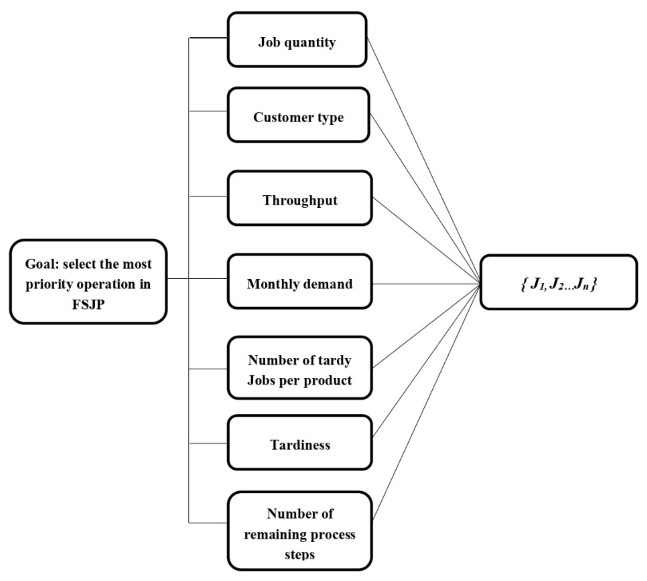
Before implementing the proposed method, it was necessary to create the MCDM model supporting the operation prioritization phase. In reply, seven job criteria or features (F1: job quantity; F2: customer type; F3: throughput; F4: monthly demand; F5: number of tardy jobs per product; F6: tardiness; and F7: number of remaining process steps) were identified.
This set of criteria (Figure 7) was pointed out considering the pertinent scientific literature and the experts’ opinion (5 production managers, 2 sales staff, the general manager, and the administrative director of the company). The experts have wide experience in production and demand management (>20 years); in addition, they have been related to the textile sector for more than 15 years and hold a professional degree in Business Administration/Industrial Engineering fields. The design of the hierarchy was led by two coauthors of this paper (MO and NJ) who have significant expertise and background in MCDM methods.
The next step was to elicit the relative priorities of each job criterion in the global decision of selecting the highest priority operation. FAHP was implemented to deal with this task considering its advantage of calculating the importance of each decision element under uncertainty. The ambiguity was incorporated in this application to obtain more realistic results given the nature of human thought and reasoning; in this case, represented by paired judgments or comparisons. In particular, the experts used the five-point scale depicted in Table A4 (Appendix A) to establish how important criterion i is with respect to criterion j when choosing the highest priority operation in FJSP. The comparisons were collected through a survey designed in a Microsoft Excel spreadsheet. The matrixes of fuzzy judgments   A ˜ K were derived for each expert using Equation (1). After this, the matrixes were aggregated by employing Equations (2) and (3). The resulting matrix A ˜ is presented in Table A5 (Appendix A). Following this, the geometric means of the fuzzy comparisons (   r ˜ i ) were calculated for each decision element (job criterion or feature) by implementing Equation (4) (Table A6).
Table A6 (Appendix A) also presents the fuzzy relative priorities of criteria ( w ˜ i ), which were achieved by using Equation (5). The fuzzy weights were then converted into crisp values using the center of area method (Equation (6)) (Table A6). These weights were normalized via applying Equation (7). The results revealed that tardiness (F6) was found to be the most important feature (GW = 0.414) when selecting the highest priority operation. This is supported by the fact that clients are more aware of being supplied in a timely manner, as previously agreed. Therefore, non-compliance with this critical factor of satisfaction may represent a potential loss of loyalty and future incomes. In fact, various competitors can take advantage of this weakness and subsequently increase their market share. This is also greatly related to the second aspect of importance in this application (number of tardy jobs per product—F5; GW= 0.203), which aims to reduce the dissatisfaction proportion of products with high expectations and background in the market. Another aspect of relevance is the throughput—F3 (GW = 0.200) of the references offered by the company. The throughput is defined as the amount of money earned by the company per time unit in the bottleneck resource; in other words, the speed at which the FJSS generates money for the firm [32,33]. In this respect, the company is interested in prioritizing those products with high throughput, which would ensure better utilization of their resources. The rest of the criteria (monthly demand, number of remaining steps, and customer type) were not found to be highly significant (GW < 0.10) on the operation selection model. On the other hand, as the CR (0.09082) was found to be less than 0.10, the matrix is concluded to be consistent, and the resulting weights are considered reliable for implementation in the practical scenario. This outcome also supports the use of a shorter version of Saaty’s scale as well as the importance of deeply understanding the hierarchy before making the comparisons. These weights (W) were later incorporated into the initial matrix X (Equation (8)) of TOPSIS application, as evidenced in Table A7 (Appendix A). This table enlists all the eligible operations in iteration 1 in conjunction with their criteria values to show an example of this procedure. In addition, the ideal ( C + ) and anti-ideal ( C ) scenarios are presented in this table according to Equations (12) and (13), correspondingly. The norm of each column was then calculated via implementing Equation (10) (Table A7). Following this, the normalized decision matrix R was achieved by using Equation (9) (Table A8 in Appendix A). Afterward, the weighted normalized decision matrix V was computed by implementing Equation (11) (Table A9, in Appendix A). The next step was to derive the Euclidean distance of each criterion to the ideal ( C + ) (Equation (14)) and anti-ideal ( C ) (Equation (15)) scenarios in each eligible operation, as observed in Table A10 and Table A11 (Appendix A), respectively.
Finally, the closeness coefficient or “priority index” of each eligible operation was computed via employing Equation (16) (Table A12 in Appendix A). In this iteration, the operation (1, 1, 9) was found to have the highest priority and had to be then chosen as the first operation to be scheduled. It is important to note that the first 6 ranked operations—CCi* > 0.5 (1,1,8; 1,1,10; 1,1,3; 1,2,8; 1,2,2; 1,1,2)—correspond to orders with the highest tardiness at the beginning of the scheduling process. This is explained by the fact that the two most relevant job features are associated with tardiness. On a different tack, the resulting schedule using the proposed DFT algorithm is shown in Table A13 (Appendix A). When contrasting the methods, we found that DFT (Test 1: −2.03 days) provides lower average lateness compared to EDD (Test 1: −0.41 days). This represents a reduction of 395.12%, which would increase the competitiveness of the smart textile company in both national and international markets. A more detailed analysis of iteration 1 is depicted in Figure 6, where we can observe that the overall DFT performance is mainly related to the orders (1,6), (3,2), (2,6), (2,1), (2,3), (1,1), and (1,7).

5. Results

According to the DFT results, the order with the earlier delivery with respect to the due date is (1,6) with 20 days in advance, while the best performance in EDD is seen in the jobs (2,2), (1,2), (1,4), and (1,6) with eight days of anticipation. In addition, the maximum lateness (13 days) is observed in (2,5) (EDD) and (1,8) (DFT). In a similar way, we can conclude that the DFT algorithm also prioritized the references with the highest throughput (3: US$1.33/min; 6: US$1.29/min; 12: US$1.27/min), which can be demonstrated through their negative lateness (Figure 8).
Furthermore, 10 iterations were carried out (including the afore-described iteration 1) to validate the general performance of the DFT and EDD models in terms of average lateness (Table A14, in Appendix A). In this case, the results confirmed that using the same set of machines, the average discrepancy between the methods is 3.86 days in favor of DFT. This was validated through a non-parametric Wilcoxon test (Table A15 in Appendix A) for paired samples (α = 0.05), which concluded that the median lateness achieved with the DFT method is significantly minor than the one provided by EDD (Z = −2.803; p-value = 0.005).

6. Conclusions

Scheduling flexible job-shop systems is a complex challenge in the context of smart manufacturing due to the dynamic and changing nature of the productive environment often characterized by a wide product portfolio, different production paths, technical restrictions, the availability of distinct technology types for the same operation, and the constant need for high customer satisfaction. In this regard, the use of integrated approaches to select operations considering different multi-criteria prioritization rules, especially in uncertain environments, can support decision-makers in the continuous improvement of the production scheduling process in FJS systems, which also contributes to bridging the existing knowledge gap referring to these applications in the smart factory industry.
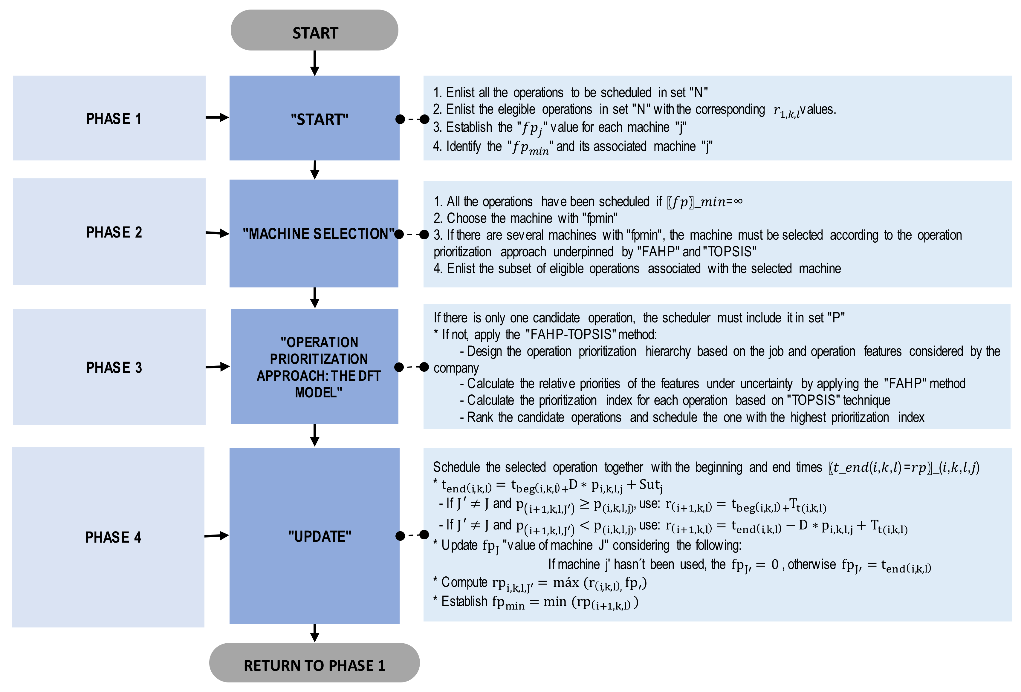
In particular, this study proposed a new framework based on the integration between the dispatching algorithm and a hybrid MCDM model composed of fuzzy AHP and TOPSIS methods to reduce the average lateness while simultaneously considering different job features of common interest for the stakeholders. The proposed DFT approach was deployed via an innovative four-phase methodology, allowing the companies to underpin the scheduling process, consider the advantages of the dispatching algorithm for addressing the FJSP and the strengths of the fuzzy multi-criteria approach to prioritize eligible operations under conditions of uncertainty, and demand changes and high product differentiation. For the development of this approach, seven criteria from market, financial, and technical domains were regarded for prioritizing the operations. Specifically, the case study here presented revealed that DFT outperformed the company’s method (EDD) by an average of 3.86 days (p-value = 0.005), while prioritizing high-throughput products for earlier delivery. The managerial and research-level implications of these outcomes extend previous studies incorporating the use of MCDM as techniques supporting the implementation of a decision support system (DSS) that facilitates the FJS scheduling operation in smart manufacturing. Future studies can consider the application of the DFT model in other FJS environments and other smart manufacturing sectors. On the other hand, maintenance restrictions and transfer batches can be incorporated to increase the robustness and applicability in the real manufacturing scenario. Additionally, there are opportunities to expand the research field upon comparing the DFT model proposed with other FJS algorithms including recent MCDM techniques like complex proportional assessment (COPRAS), best–worst method (BWM), and intuitionistic fuzzy AHP (IF-AHP) so that improvements on average lateness and other key performance measures can be achieved.

Author Contributions

Writing—original draft, M.O.-B., A.P., F.D.F., N.J.-R., G.J.-D., and L.B.-L. All authors have read and agreed to the published version of the manuscript.

Funding

This research received no external funding.

Institutional Review Board Statement

Not applicable.

Informed Consent Statement

Not applicable.

Data Availability Statement

Not applicable.

Conflicts of Interest

The authors declare no conflict of interest.

Nomenclature

r number of references
n number of jobs
m number of machines
D job quantity
j machine associated with the next operation in job route
r i , k , l release time of operation i associated with job k of product reference l
p i , k , l , j processing time of operation i associated with job k of product reference l
f p j time in which the machine j is ready to process a new operation
t b e g i , k , l beginning time of operation i associated with job k of product reference l
t e n d i , k , l end time of operation i associated with job k of product reference l
r p i , k , l ,   j earlier ready time of operation i associated with job k of product reference l and whose execution is to be scheduled in machine j
S U t j setup time in machine j
T t i , k , l transfer time of operation i associated with job k of product reference l

Appendix A

Table A1. Processing times for each product reference in each machine.
PROCESSWeavingDyeingPrintingCuttingWhipstitchingCleaning
Product/ResourceT1T2T3C1C2C3C4ECTCP1CP2LP1LP2
Single coloured bedcover164.421020433.636.65436-29.4606025.825.8
Single fringe coloured bedcover--16540.243.864.843.2-29.4606025.825.8
Stamped single bedcover164.421020433.636.6543656.429.4606025.825.8
Double coloured bedcover253.8-230.46671.4106.270.8-29.479.879.832.432.4
Double fringe coloured bedcover--394.250.455.28153.4-29.479.879.832.432.4
Stamped double bedcover253.8-230.46671.4106.270.89029.479.879.832.432.4
Special single coloured bedcover--2163336.653.435.4-30.6303025.825.8
Special single fringe coloured bedcover--16240.243.864.242.6-30.6303025.825.8
Special double coloured bedcover--194.440.243.864.242.6-30.6303025.825.8
Special double fringe coloured bedcover--260.440.243.864.242.6-30.6303025.825.8
Smooth poncho44.4-51.6-----7.252.252.28484
White poncho-45.651.6-----7.252.252.28484
White mulera256.8-298.8-----2.452.252.2262.2262.2
Table A2. Demand schedule and characterization of orders in terms of throughput, monthly demand, quantity, due date, DOT, and % of tardiness.
ProductThroughputM.DJobsTotal% of Tardiness
Job 1Job 2Job 3Job 4
UnitsDelivery DateD.O.T.UnitsDelivery DateD.O.T.UnitsDelivery DateUnitsDelivery Date
Single coloured bedcover0.99230094415-feb-94528-feb-----18890
Single fringe coloured bedcover0.9914005425-gen610825-gen6128415-feb128528-feb27315.9
Stamped single bedcover1.33120314221-gen107015-feb-7128-feb--28350.1
Double coloured bedcover0.97120017426-gen587715-feb-87728-feb--19289.1
Double fringe coloured bedcover0.6250097715-feb-97728-feb-----19540
Stamped double bedcover1.291872427-gen43628-gen36415-feb6428-feb18831.9
Special single coloured bedcover1.0120428815-feb-8828-feb-----1760
Special single fringe coloured bedcover1.0130510419-gen1210825-gen6----212100
Special double coloured bedcover0.7620425028-feb--------500
Special doublé fringe coloured bedcover0.6130958422-gen914015-feb-14028-feb--86467.5
Smooth poncho1.051488225008-feb--------22500
White poncho1.271488595016-feb--------59500
White mulera0.443250200018-feb--------20000
Table A3. Customer type and order quantity.
Product ReferenceQuantity (Units)Customer Type
Single colored bedcover9444
9451
Single fringe colored bedcover542
1082
12842
12854
Stamped single bedcover1422
704
711
Double colored bedcover1744
8774
8774
Double fringe colored bedcover9771
9774
Stamped double bedcover243
361
641
642
Special single colored bedcover885
885
Special single fringe colored bedcover1045
1085
Special double colored bedcover501
Special double fringe colored bedcover5844
1403
1402
Smooth poncho22502
White poncho59505
White mulera2001
Table A4. Setup times and available resources.
ItemOperation (Resources)Setup Time (min)
Single colored bedcoverWeaving (T1, T2, T3)50
Dyeing (C1, C2, C3, C4)50
Cutting (CT)2.5
Whipstitching (CP1, CP2)5
Cleaning (LP1, LP2)1
Single fringe colored bedcoverWeaving (T3)65
Dyeing (C1, C2, C3, C4)50
Cutting (CT)2.5
Whipstitching (CP1, CP2)5
Cleaning (LP1, LP2)1
Stamped single bedcoverWeaving (T1, T2, T3)50
Dyeing (C1, C2, C3, C4)120
Printing (E)50
Cutting (CT)2.5
Whipstitching (CP1, CP2)5
Cleaning (LP1, LP2)1
Double colored bedcoverWeaving (T1, T3)90
Dyeing (C1, C2, C3, C4)60
Cutting (CT)4
Whipstitching (CP1, CP2)5.2
Cleaning (LP1, LP2)1.5
Double fringe colored bedcoverWeaving (T3)105
Dyeing (C1, C2, C3, C4)60
Cutting (CT)4
Whipstitching (CP1, CP2)5.2
Cleaning (LP1, LP2)1.5
Stamped double bedcoverWeaving (T1, T3)90
Dyeing (C1, C2, C3, C4)60
Printing (E)70
Cutting (CT)4
Whipstitching (CP1, CP2)5.2
Cleaning (LP1, LP2)1.5
Special single colored bedcoverWeaving (T3)60
Dyeing (C1, C2, C3, C4)60
Cutting (CT)2.5
Whipstitching (CP1, CP2)5
Cleaning (LP1, LP2)1
Special single fringe colored bedcoverWeaving (T3)75
Dyeing (C1, C2, C3, C4)60
Cutting (CT)2.5
Whipstitching (CP1, CP2)5
Cleaning (LP1, LP2)1
Special double colored bedcoverWeaving (T3)105
Dyeing (C1, C2, C3, C4)70
Cutting (CT)3.5
Whipstitching (CP1, CP2)5.5
Cleaning (LP1, LP2)2
Special double fringe colored bedcoverWeaving (T3)120
Dyeing (C1,C2, C3,C4)70
Cutting (CT)3.5
Whipstitching (CP1, CP2)5.5
Cleaning (LP1, LP2)2
Smooth ponchoWeaving (T1, T3)30
Cutting (CT)1.5
Whipstitching (CP1, CP2)4.5
Cleaning (LP1, LP2)1
White ponchoWeaving (T2, T3)30
Cutting (CT)1.5
Whipstitching (CP1, CP2)4.5
Cleaning (LP1, LP2)1
White muleraWeaving (T1, T3)30
Cutting (CT)1.5
Whipstitching (CP1, CP2)4.5
Cleaning (LP1, LP2)1
Table A5. The aggregated matrix of fuzzy comparisons A ˜ .
F1F2F3F4F5F6F7
F1[1,1,1][1,1,1][0.16,0.2,0.25][2,3,4][0.25,0.33,0.5][0.16,0.2,0.25][2,3,4]
F2[1,1,1][1,1,1][0.16,0.2,0.25][2,3,4][0.16,0.2,0.25][0.16,0.2,0.25][2,3,4]
F3[4,5,6][4,5,6][1,1,1][4,5,6][1,1,1][0.16,0.2,0.25][4,5,6]
F4[0.25,0.33,0.5][0.25,0.33,0.5][0.16,0.2,0.25][1,1,1][0.16,0.2,0.25][0.16,0.2,0.25][2,3,4]
F5[2,3,4][4,5,6][1,1,1][4,5,6][1,1,1][0.25,0.33,0.5][4,5,6]
F6[4,5,6][4,5,6][4,5,6][4,5,6][2,3,4][1,1,1][4,5,6]
F7[0.25,0.33,0.5][0.25,0.33,0.5][0.16,0.2,0.25][0.25,0.33,0.5][0.16,0.2,0.25][0.16,0.2,0.25][1,1,1]
Table A6. The geometric means of fuzzy comparisons for job features, fuzzy weights, non-fuzzy weights, and crisp weights.
CriterionGeometric Mean of Fuzzy ComparisonsFuzzy WeightNon-Fuzzy WeightNorm Weight
F10.540.700.890.040.060.100.070.064
F20.500.640.790.040.060.090.060.058
F31.862.242.620.130.200.290.210.200
F40.280.370.500.020.030.060.040.035
F51.782.232.750.120.200.300.210.203
F63.564.595.610.250.410.620.430.414
F70.200.260.350.010.020.040.030.025
Total8.7311.0313.52 Total1.03
Reverse0.110.090.07
Increasing order0.070.090.11
Table A7. The initial decision matrix X in TOPSIS application—1st iteration.
F1F2F3F4F5F6F7
(1,1,1)94440.9902300005
(1,2,1)94510.9902300005
(1,1,2)5420.9901400265
(1,2,2)10820.9901400265
(1,3,2)128420.9901400205
(1,4,2)128540.9901400205
(1,1,3)14221.33012031106
(1,2,3)7041.3301203106
(1,3,3)7111.3301203106
(1,1,4)17440.9701200155
(1,2,4)87740.9701200105
(1,3,4)87740.9701200105
(1,1,5)97710.620500005
(1,2,5)97740.620500005
(1,1,6)2431.290187246
(1,2,6)3611.290187236
(1,3,6)6411.290187206
(1,4,6)6421.290187206
(1,1,7)8851.0102042005
(1,2,7)8851.0102042005
(1,1,8)10451.0103052125
(1,2,8)10851.010305265
(1,1,9)5010.7602042005
(1,1,10)58440.610309195
(1,2,10)14030.610309105
(1,3,10)14020.610309105
(1,1,11)225021.0501488004
(1,1,12)595051.2701488004
(1,1,13)200010.4403250004
C+595051.33032502101
C2410.440187006
W0.0640.0580.2000.0350.2030.4140.025
Norm7,314,51317,49354887,462,846700021,97727,839
Table A8. The normalized decision matrix R in TOPSIS application—1st iteration.
F1F2F3F4F5F6F7
(1,1,1)0.1290.2290.1800.3080.0000.0000.180
(1,2,1)0.1290.0570.1800.3080.0000.0000.180
(1,1,2)0.0070.1140.1800.1880.2860.2730.180
(1,2,2)0.0150.1140.1800.1880.2860.2730.180
(1,3,2)0.1760.1140.1800.1880.2860.0000.180
(1,4,2)0.1760.2290.1800.1880.2860.0000.180
(1,1,3)0.0190.1140.2420.1610.1430.4550.216
(1,2,3)0.0100.2290.2420.1610.1430.0000.216
(1,3,3)0.0100.0570.2420.1610.1430.0000.216
(1,1,4)0.0240.2290.1770.1610.1430.2270.180
(1,2,4)0.1200.2290.1770.1610.1430.0000.180
(1,3,4)0.1200.2290.1770.1610.1430.0000.180
(1,1,5)0.1340.0570.1130.0670.0000.0000.180
(1,2,5)0.1340.2290.1130.0670.0000.0000.180
(1,1,6)0.0030.1710.2350.0250.2860.1820.216
(1,2,6)0.0050.0570.2350.0250.2860.1360.216
(1,3,6)0.0090.0570.2350.0250.2860.0000.216
(1,4,6)0.0090.1140.2350.0250.2860.0000.216
(1,1,7)0.0120.2860.1840.2740.0000.0000.180
(1,2,7)0.0120.2860.1840.2740.0000.0000.180
(1,1,8)0.0140.2860.1840.0410.2860.5460.180
(1,2,8)0.0150.2860.1840.0410.2860.2730.180
(1,1,9)0.0070.0570.1380.2740.0000.0000.180
(1,1,10)0.0800.2290.1110.0410.1430.4090.180
(1,2,10)0.0190.1710.1110.0410.1430.0000.180
(1,3,10)0.0190.1140.1110.0410.1430.0000.180
(1,1,11)0.3080.1140.1910.1990.0000.0000.144
(1,1,12)0.8130.2860.2310.1990.0000.0000.144
(1,1,13)0.2730.0570.0800.4350.0000.0000.144
A+0.8130.2860.2420.4350.2860.5460.036
A0.0030.0570.0800.0250.0000.0000.216
W0.0640.0580.2000.0350.2030.4140.025
Table A9. The weighted normalized decision matrix V in TOPSIS application—1st iteration.
F1F2F3F4F5F6F7
(1,1,1)0.0080.0130.0360.0110.0000.0000.004
(1,2,1)0.0080.0030.0360.0110.0000.0000.004
(1,1,2)0.0000.0070.0360.0070.0580.1130.004
(1,2,2)0.0010.0070.0360.0070.0580.1130.004
(1,3,2)0.0110.0070.0360.0070.0580.0000.004
(1,4,2)0.0110.0130.0360.0070.0580.0000.004
(1,1,3)0.0010.0070.0480.0060.0290.1880.005
(1,2,3)0.0010.0130.0480.0060.0290.0000.005
(1,3,3)0.0010.0030.0480.0060.0290.0000.005
(1,1,4)0.0020.0130.0350.0060.0290.0940.004
(1,2,4)0.0080.0130.0350.0060.0290.0000.004
(1,3,4)0.0080.0130.0350.0060.0290.0000.004
(1,1,5)0.0090.0030.0230.0020.0000.0000.004
(1,2,5)0.0090.0130.0230.0020.0000.0000.004
(1,1,6)0.0000.0100.0470.0010.0580.0750.005
(1,2,6)0.0000.0030.0470.0010.0580.0570.005
(1,3,6)0.0010.0030.0470.0010.0580.0000.005
(1,4,6)0.0010.0070.0470.0010.0580.0000.005
(1,1,7)0.0010.0170.0370.0100.0000.0000.004
(1,2,7)0.0010.0170.0370.0100.0000.0000.004
(1,1,8)0.0010.0170.0370.0010.0580.2260.004
(1,2,8)0.0010.0170.0370.0010.0580.1130.004
(1,1,9)0.0000.0030.0280.0100.0000.0000.004
(1,1,10)0.0050.0130.0220.0010.0290.1700.004
(1,2,10)0.0010.0100.0220.0010.0290.0000.004
(1,3,10)0.0010.0070.0220.0010.0290.0000.004
(1,1,11)0.0200.0070.0380.0070.0000.0000.004
(1,1,12)0.0520.0170.0460.0070.0000.0000.004
(1,1,13)0.0170.0030.0160.0150.0000.0000.004
A+0.0520.0170.0480.0150.0580.2260.001
A-0.0000.0030.0160.0010.0000.0000.005
Table A10. Total separation of eligible operations from the ideal scenario—1st iteration.
F1F2F3F4F5F6F7Si+
(1,1,1)0.0020.0000.0000.0000.0030.0510.0000.238
(1,2,1)0.0020.0000.0000.0000.0030.0510.0000.238
(1,1,2)0.0030.0000.0000.0000.0000.0130.0000.126
(1,2,2)0.0030.0000.0000.0000.0000.0130.0000.125
(1,3,2)0.0020.0000.0000.0000.0000.0510.0000.230
(1,4,2)0.0020.0000.0000.0000.0000.0510.0000.230
(1,1,3)0.0030.0000.0000.0000.0010.0010.0000.071
(1,2,3)0.0030.0000.0000.0000.0010.0510.0000.234
(1,3,3)0.0030.0000.0000.0000.0010.0510.0000.234
(1,1,4)0.0030.0000.0000.0000.0010.0170.0000.145
(1,2,4)0.0020.0000.0000.0000.0010.0510.0000.233
(1,3,4)0.0020.0000.0000.0000.0010.0510.0000.233
(1,1,5)0.0020.0000.0010.0000.0030.0510.0000.240
(1,2,5)0.0020.0000.0010.0000.0030.0510.0000.239
(1,1,6)0.0030.0000.0000.0000.0000.0230.0000.160
(1,2,6)0.0030.0000.0000.0000.0000.0290.0000.178
(1,3,6)0.0030.0000.0000.0000.0000.0510.0000.233
(1,4,6)0.0030.0000.0000.0000.0000.0510.0000.233
(1,1,7)0.0030.0000.0000.0000.0030.0510.0000.239
(1,2,7)0.0030.0000.0000.0000.0030.0510.0000.239
(1,1,8)0.0030.0000.0000.0000.0000.0000.0000.054
(1,2,8)0.0030.0000.0000.0000.0000.0130.0000.125
(1,1,9)0.0030.0000.0000.0000.0030.0510.0000.240
(1,1,10)0.0020.0000.0010.0000.0010.0030.0000.085
(1,2,10)0.0030.0000.0010.0000.0010.0510.0000.236
(1,3,10)0.0030.0000.0010.0000.0010.0510.0000.236
(1,1,11)0.0010.0000.0000.0000.0030.0510.0000.236
(1,1,12)0.0000.0000.0000.0000.0030.0510.0000.234
(1,1,13)0.0010.0000.0010.0000.0030.0510.0000.239
Table A11. Total separation of eligible operations from the anti-ideal scenario—1st iteration.
F1F2F3F4F5F6F7Si
(1,1,1)0.0000.0000.0000.0000.0000.0000.0000.026
(1,2,1)0.0000.0000.0000.0000.0000.0000.0000.024
(1,1,2)0.0000.0000.0000.0000.0030.0130.0000.129
(1,2,2)0.0000.0000.0000.0000.0030.0130.0000.129
(1,3,2)0.0000.0000.0000.0000.0030.0000.0000.063
(1,4,2)0.0000.0000.0000.0000.0030.0000.0000.063
(1,1,3)0.0000.0000.0010.0000.0010.0350.0000.193
(1,2,3)0.0000.0000.0010.0000.0010.0000.0000.045
(1,3,3)0.0000.0000.0010.0000.0010.0000.0000.044
(1,1,4)0.0000.0000.0000.0000.0010.0090.0000.101
(1,2,4)0.0000.0000.0000.0000.0010.0000.0000.037
(1,3,4)0.0000.0000.0000.0000.0010.0000.0000.037
(1,1,5)0.0000.0000.0000.0000.0000.0000.0000.011
(1,2,5)0.0000.0000.0000.0000.0000.0000.0000.015
(1,1,6)0.0000.0000.0010.0000.0030.0060.0000.100
(1,2,6)0.0000.0000.0010.0000.0030.0030.0000.087
(1,3,6)0.0000.0000.0010.0000.0030.0000.0000.066
(1,4,6)0.0000.0000.0010.0000.0030.0000.0000.066
(1,1,7)0.0000.0000.0000.0000.0000.0000.0000.026
(1,2,7)0.0000.0000.0000.0000.0000.0000.0000.026
(1,1,8)0.0000.0000.0000.0000.0030.0510.0000.235
(1,2,8)0.0000.0000.0000.0000.0030.0130.0000.129
(1,1,9)0.0000.0000.0000.0000.0000.0000.0000.015
(1,1,10)0.0000.0000.0000.0000.0010.0290.0000.172
(1,2,10)0.0000.0000.0000.0000.0010.0000.0000.030
(1,3,10)0.0000.0000.0000.0000.0010.0000.0000.030
(1,1,11)0.0000.0000.0000.0000.0000.0000.0000.030
(1,1,12)0.0030.0000.0010.0000.0000.0000.0000.062
(1,1,13)0.0000.0000.0000.0000.0000.0000.0000.023
Table A12. Priority index of eligible operations—1st iteration.
Candidate Operation C C i Candidate Operation C C i
(1,1,8)0.8119(1,3,3)0.1574
(1,1,3)0.7312(1,2,4)0.1381
(1,1,10)0.6711(1,3,4)0.1381
(1,2,8)0.5079(1,2,10)0.1144
(1,2,2)0.5066(1,1,11)0.1141
(1,1,2)0.5062(1,3,10)0.1125
(1,1,4)0.4104(1,1,7)0.0985
(1,1,6)0.3848(1,2,7)0.0985
(1,2,6)0.3271(1,1,1)0.0978
(1,4,6)0.2206(1,2,1)0.0908
(1,3,6)0.2203(1,1,13)0.0864
(1,4,2)0.2159(1,2,5)0.0577
(1,3,2)0.2139(1,1,9)0.0572
(1,1,12)0.2093(1,1,5)0.0429
(1,2,3)0.1610
Table A13. Schedule resulting from the DFT algorithm.
Scheduled OperationMachineT. Beginning (min)T. End (min)
(1,1,8)T30.0355.8
(2,1,8)C1357.8487.5
(4,1,8)CT489.5545.0
(5,1,8)CP1547.0604.0
(6,1,8)LP1606.0651.7
(1,1,3)T10.0439.1
(2,1,3)C4441.1646.3
(3,1,3)E648.3831.8
(4,1,3)CT833.8905.8
(5,1,3)CP2907.81054.8
(6,1,3)LP21056.81118.9
(1,1,10)T3355.82368.0
(2,1,10)C12370.02831.2
(4,1,10)CT2833.23134.6
(5,1,10)CP13136.63434.1
(6,1,10)LP13436.13689.2
(1,2,8)T32368.02734.6
(2,2,8)C12736.62868.9
(4,2,8)CT3134.63192.2
(5,2,8)CP23194.23253.2
(6,2,8)LP23255.23302.6
(1,2,2)T32734.63096.6
(2,2,2)C13098.63220.9
(4,2,2)CT3222.93278.3
(5,2,2)CP23280.33393.3
(6,2,2)LP23395.33442.8
(1,1,2)T33096.63310.1
(2,1,2)C13312.13398.2
(4,1,2)CT3400.23429.2
(5,1,2)CP23431.23490.2
(6,1,2)LP23492.23516.4
(1,1,4)T1439.11265.1
(2,1,4)C41267.11532.4
(4,1,4)CT3429.23518.5
(5,1,4)CP13520.53757.1
(6,1,4)LP23759.13854.5
(1,1,6)T11265.11456.6
(2,1,6)C21458.61547.2
(3,1,6)E1549.21655.2
(4,1,6)CT3518.53534.2
(5,1,6)CP23536.23573.3
(6,1,6)LP13689.23703.7
(1,2,6)T11456.61698.9
(2,2,6)C41700.91803.4
(3,2,6)E1805.41929.4
(4,2,6)CT3534.23555.9
(5,2,6)CP23573.33626.4
(6,2,6)LP13703.73724.6
(1,4,2)T33310.16908.8
(2,4,2)C16910.87821.8
(4,4,2)CT7823.88455.9
(5,4,2)CP28457.99747.9
(6,4,2)LP19749.910,303.5
(1,3,2)T36908.810,504.8
(2,3,2)C110,506.811,417.1
(4,3,2)CT11,419.112,050.8
(5,3,2)CP112,052.813,341.8
(6,3,2)LP213,343.813,896.9
(1,4,6)T11698.92059.6
(2,4,6)C42061.62197.1
(3,4,6)E2199.12365.1
(4,4,6)CT12,050.812,086.1
(5,4,6)CP212,088.112,178.4
(6,4,6)LP112,180.412,216.5
(1,3,6)T12059.62420.3
(2,3,6)C42422.32557.9
(3,3,6)E2559.92725.9
(4,3,6)CT12,086.112,121.5
(5,3,6)CP212,178.412,268.8
(6,3,6)LP112,270.812,306.8
(1,2,3)T20.0295.0
(2,2,3)C3297.0480.0
(1,3,3)T2295.0593.5
(2,3,3)C3595.5779.4
(1,1,12)T2593.55145.5
(1,2,4)T12420.36220.1
(2,2,4)C46222.17316.9
(3,2,3)E2725.92841.7
(3,3,3)E2841.72958.4
(1,1,1)T25145.58499.5
(2,1,1)C48499.59115.9
(1,3,4)T16220.110,019.8
(2,3,4)C410,021.811,116.6
(1,2,1)T28499.511,857.0
(2,2,1)C211,859.012,485.5
(1,1,11)T110,019.811,714.8
(1,2,10)T310,504.811,078.4
(1,3,10)T311,078.411,652.0
(2,2,10)C411,116.611,286.0
(2,3,10)C411,654.011,823.4
(1,1,7)T311,652.012,028.8
(2,1,7)C112,030.812,139.2
(1,1,13)T111,714.820,304.8
(1,2,7)T312,028.812,405.6
(2,2,7)C412,407.612,519.5
(1,1,9)T312,405.612,672.6
(2,1,9)C112,674.612,778.1
(4,2,3)CT12,121.512,158.3
(4,3,3)CT12,158.312,195.6
(4,2,4)CT12,195.612,629.3
(5,2,3)CP212,268.812,343.8
(6,2,3)LP112,345.812,376.9
(5,3,3)CP212,343.812,419.8
(6,3,3)LP112,421.812,453.3
(5,2,4)CP212,631.313,802.9
(6,2,4)LP113,804.914,280.0
(4,3,4)CT12,629.313,063.0
(1,2,5)T312,672.619,196.5
(2,2,5)C219,198.520,157.3
(4,2,10)CT13,063.013,137.9
(4,3,10)CT13,137.913,212.8
(4,1,12)CT13,212.813,928.3
(5,3,4)CP113,341.814,513.4
(5,2,10)CP213,802.913,878.4
(5,3,10)CP213,878.413,953.9
(6,3,4)LP214,515.414,990.4
(4,1,11)CT13,928.314,199.8
(5,1,12)CP213,953.919,134.9
(4,1,7)CT14,199.814,247.2
(4,2,7)CT14,247.214,294.6
(6,2,10)LP114,280.014,342.2
(4,1,1)CT14,294.614,759.6
(6,3,10)LP114,342.214,404.4
(6,1,12)LP119,134.927,465.9
(5,1,11)CP114,513.416,475.4
(4,2,1)CT14,759.615,225.2
(6,1,11)LP216,477.419,628.4
(4,1,13)CT20,306.820,388.3
(5,1,7)CP116,475.416,524.4
(5,1,1)CP116,524.417,473.4
(5,2,7)CP117,473.417,522.4
(5,2,1)CP117,522.418,472.4
(5,1,13)CP120,390.322,134.8
(1,1,5)T319,196.525,720.4
(2,1,5)C125,722.426,603.1
(6,1,1)LP219,628.420,035.3
(6,1,7)LP220,035.320,074.1
(6,2,7)LP220,074.120,113.0
(6,2,1)LP220,113.020,520.3
(4,2,5)CT20,388.320,871.0
(6,1,13)LP222,136.830,877.8
(5,2,5)CP220,873.022,177.6
(4,1,5)CT26,605.127,087.8
(5,1,5)CP127,089.828,394.4
(4,1,9)CT27,087.827,116.8
(5,1,9)CP227,118.827,149.3
(6,2,5)LP127,465.927,995.0
(6,1,5)LP128,396.428,925.5
(6,1,9)LP128,925.528,949.0
Table A14. Comparative analysis between DFT and EDD in terms of average lateness.
Test NumberAverage Lateness (Days/Order)Discrepancy (Days)
DFTEDD
1−2.03−0.41−1.62
2−4.03−2.60−1.43
31.803.76−1.96
4−1.91−0.11−1.80
55.288.34−3.06
61.445.06−3.62
76.8811.06−4.18
8−0.065.53−5.59
98.4516.12−7.67
100.478.19−7.72
Table A15. Comparative analysis between DFT and EDD in terms of average lateness.
EDD-DFT NAverage RangeRange Sum
Negative ranges00.000.00
Positive ranges105.5055.00
Draws0Zp-value
Total10−2.8030.005

References

  1. Fu, Y.; Hou, Y.; Wang, Z.; Gao, K.; Wang, L. Distributed scheduling problems in intelligent manufacturing systems. Tsinghua Sci. Technol. 2021, 26, 625–645. [Google Scholar] [CrossRef]
  2. Rahman, H.F.; Janardhanan, M.N.; Chuen, L.P.; Ponnambalam, S.G. Flowshop scheduling with sequence dependent setup times and batch delivery in supply chain. Comput. Ind. Eng. 2021, 158, 107378. [Google Scholar] [CrossRef]
  3. Hakeem-Ur-Rehman; Wan, G.; Zhan, Y. Multi-level, multi-stage lot-sizing and scheduling in the flexible flow shop with demand information updating. Int. Trans. Oper. Res. 2021, 28, 2191–2217. [Google Scholar] [CrossRef]
  4. Khalid, Q.S.; Azim, S.; Abas, M.; Babar, A.R.; Ahmad, I. Modified particle swarm algorithm for scheduling agricultural products. Eng. Sci. Technol. Int. J. 2021, 24, 818–828. [Google Scholar]
  5. De Lacalle, L.N.L.; Lamikiz, A.; Salgado, M.A.; Herranz, S.; Rivero, A. Process planning for reliable high-speed machining of moulds. Int. J. Prod. Res. 2002, 40, 2789–2809. [Google Scholar] [CrossRef]
  6. Che, Y.; Hu, K.; Zhang, Z.; Lim, A. Machine scheduling with orientation selection and two-dimensional packing for additive manufacturing. Comput. Oper. Res. 2021, 130, 105245. [Google Scholar] [CrossRef]
  7. Lamikiz, A.; de Lacalle, L.N.L.; Sánchez, J.A.; Salgado, M.A. Cutting force integration at the CAM stage in the high-speed milling of complex surfaces. Int. J. Comput. Integr. Manuf. 2005, 18, 586–600. [Google Scholar] [CrossRef]
  8. Wang, C.; Li, Y.; Li, X. Solving flexible job shop scheduling problem by a multi-swarm collaborative genetic algorithm. J. Syst. Eng. Electron. 2021, 32, 261–271. [Google Scholar]
  9. Sangaiah, A.K.; Suraki, M.Y.; Sadeghilalimi, M.; Hosseinabadi, A.A.R.; Wang, J. A new meta-heuristic algorithm for solving the flexible dynamic job-shop problem with parallel machines. Symmetry 2019, 11, 165. [Google Scholar] [CrossRef] [Green Version]
  10. Vargas, J.; Calvo, R. Joint optimization of process flow and scheduling in service-oriented manufacturing systems. Materials 2018, 11, 1559. [Google Scholar] [CrossRef] [Green Version]
  11. Fattahi, P.; Fallahi, A. Dynamic scheduling in flexible job shop systems by considering simultaneously efficiency and stability. CIRP J. Manuf. Sci. Technol. 2020, 2, 114–123. [Google Scholar] [CrossRef]
  12. Wu, Z.; Weng, M.X. Multiagent scheduling method with earliness and tardiness objectives in flexible job shops. IEEE Trans. Syst. Man Cybern. Part B Cybern. 2005, 35, 293–301. [Google Scholar] [CrossRef]
  13. Červeňanská, Z.; Važan, P.; Juhás, M.; Juhásová, B. Multi-criteria optimization in operations scheduling applying selected priority rules. Appl. Sci. 2021, 11, 2783. [Google Scholar] [CrossRef]
  14. Sun, L.; Lin, L.; Gen, M.; Li, H. A hybrid cooperative coevolution algorithm for fuzzy flexible job shop scheduling. IEEE Trans. Fuzzy Syst. 2019, 27, 1008–1022. [Google Scholar] [CrossRef]
  15. Gen, M.; Lin, L.; Zhang, W. Multiobjective hybrid genetic algorithms for manufacturing scheduling: Part I models and algorithms. Adv. Intell. Syst. Comput. 2015, 362, 3–25. [Google Scholar]
  16. Li, Y.; Carabelli, S.; Fadda, E.; Tadei, R.; Terzo, O. Machine learning and optimization for production rescheduling in Industry 4.0. Int. J. Adv. Manuf. Technol. 2020, 110, 2445–2463. [Google Scholar] [CrossRef]
  17. Ghaleb, M.; Zolfagharinia, H.; Taghipour, S. Real-time production scheduling in the Industry-4.0 context: Addressing uncertainties in job arrivals and machine breakdowns. Comput. Oper. Res. 2020, 123, 105031. [Google Scholar] [CrossRef]
  18. Mihoubi, B.; Bouzouia, B.; Gaham, M. Reactive scheduling approach for solving a realistic flexible job shop scheduling problem. Int. J. Prod. Res. 2020, 1–19. [Google Scholar] [CrossRef]
  19. Lim, C.H.; Moon, S.K.; Okpoti, E.S. A Reusable Scheduling Problem Decomposition Framework for Smart Factories. In Proceedings of the IEEE International Conference on Industrial Engineering and Engineering Management, Macao, China, 15–18 December 2019; pp. 516–520. [Google Scholar]
  20. Vazan, P.; Cervenanska, Z.; Kotianova, J.; Krizanova, G. The impact of selected priority rules on production goals. In Proceedings of the 2019 20th International Carpathian Control Conference, Krakow-Wieliczka, Poland, 26–29 May 2019. [Google Scholar]
  21. Ma, A.; Nassehi, A.; Snider, C. Anarchic manufacturing. Int. J. Prod. Res. 2019, 57, 2514–2530. [Google Scholar] [CrossRef] [Green Version]
  22. Dolgui, A.; Ivanov, D.; Sethi, S.P.; Sokolov, B. Scheduling in production, supply chain and Industry 4.0 systems by optimal control: Fundamentals, state-of-the-art and applications. Int. J. Prod. Res. 2019, 57, 411–432. [Google Scholar] [CrossRef]
  23. Heger, J.; Voß, T. Dynamic priority based dispatching of AGVs in flexible job shops. Procedia CIRP 2019, 79, 445–449. [Google Scholar] [CrossRef]
  24. Murín, S.; Rudová, H. Scheduling of Mobile Robots Using Constraint Programming. Lect. Notes Comput. Sci. 2019, 456–471. [Google Scholar]
  25. Kim, J.W.; Kim, S.K. Interactive job sequencing system for small make-to-order manufacturers under smart manufacturing environment. Peer Peer Netw. Appl. 2019. [Google Scholar] [CrossRef]
  26. Alves, F.; Varela, M.L.R.; Rocha, A.M.A.C.; Pereira, A.I.; Leitão, P. A human centred hybrid MAS and meta-heuristics based system for simultaneously supporting scheduling and plant layout adjustment. FME Trans. 2019, 47, 699–710. [Google Scholar] [CrossRef] [Green Version]
  27. Gozali, L.; Kurniawan, V.; Nasution, S.R. Design of Job Scheduling System and Software for Packaging Process with SPT. EDD. LPT. CDS and NEH algorithm at PT. ACP. IOP Conf. Ser. Mater. Sci. Eng. 2019, 528, 012045. [Google Scholar] [CrossRef]
  28. Lunardi, W.T.; Voos, H.; Cherri, L.H. An Imperialist Competitive Algorithm for a Real-World Flexible Job Shop Scheduling Problem. In Proceedings of the IEEE International Conference on Emerging Technologies and Factory Automation, ETFA, Turin, Italy, 4–7 September 2018; pp. 402–409. [Google Scholar]
  29. Ortíz-Barrios, M.; Neira-Rodado, D.; Jiménez-Delgado, G.; Hernández-Palma, H. Using fahp-vikor for operation selection in the flexible job-shop scheduling problem: A case study in textile industry. Lect. Notes Comput. Sci. 2018. [Google Scholar] [CrossRef]
  30. Wang, C.; Jiang, P.; Lu, T. The production instruction system for smart job shop. In Proceedings of the IEEE International Conference on Mechatronics and Automation, Harbin, China, 7–10 August 2016; pp. 1850–1854. [Google Scholar]
  31. Bouazza, W.; Sallez, Y.; Beldjilali, B. A distributed approach solving partially flexible job-shop scheduling problem with a Q-learning effect. IFAC PapersOnLine 2017, 50, 15890–15895. [Google Scholar] [CrossRef]
  32. Ivanov, D.; Dolgui, A.; Sokolov, B. A Dynamic Approach to Multi-stage Job Shop Scheduling in an Industry 4.0-Based Flexible Assembly System. IFIP Adv. Inf. Commun. Technol. 2017, 513, 475–482. [Google Scholar]
  33. Son, D.S.; Lee, Y.H.; Shin, Y.W.; Moon, D.H. A simulation study on a flexible manufacturing systems for producing aircraft engine parts (WIP). Simul. Ser. 2017, 49, 205–210. [Google Scholar]
  34. Yuan, G.C.; Bao, J.S.; Zhang, Q.W.; Li, Z.Q. An intelligent scheduling method for manufacturing system based on M2M. In Proceedings of the International Conference on Computers and Industrial Engineering, CIE, Lisbon, Portugal, 11–13 October 2017. [Google Scholar]
  35. Jacob, E.; Astorga, J.; Unzilla, J.J.; García, D.; López-De-Lacalle, L.N. Towards a 5G compliant and flexible connected manufacturing facility | [Hacia una infraestructura de fabricación flexible, conectada e integrable en redes 5G]. Dyna 2018, 93, 656–662. [Google Scholar] [CrossRef] [Green Version]
  36. Tian, S.; Wang, T.; Zhang, L.; Wu, X. The Internet of Things enabled manufacturing enterprise information system design and shop floor dynamic scheduling optimisation. Enterp. Inf. Syst. 2020, 14, 1238–1263. [Google Scholar] [CrossRef]
  37. Zhao, F.; Hong, Y.; Yu, D.; Yang, Y.; Zhang, Q. A hybrid particle swarm optimisation algorithm and fuzzy logic for process planning and production scheduling integration in holonic manufacturing systems. Int. J. Comput. Integr. Manuf. 2010, 23, 20–39. [Google Scholar] [CrossRef]
  38. Chen, Y.; Huang, C.; Chou, F.-D.; Huang, S. Single-machine scheduling problem with flexible maintenance and non-resumable jobs to minimise makespan. IET Collab. Intell. Manuf. 2020, 2, 174–181. [Google Scholar] [CrossRef]
  39. Paprocka, I.; Kampa, A.; Gołda, G. The effects of a machine failure on the robustness of job shop systems-the predictive-reactive approach. Int. J. Mod. Manuf. Technol. 2019, 11, 72–79. [Google Scholar]
  40. Kaya, İ.; Erdoğan, M.; Karaşan, A.; Özkan, B. Creating a road map for industry 4.0 by using an integrated fuzzy multicriteria decision-making methodology. Soft Comput. 2020, 24, 17931–17956. [Google Scholar] [CrossRef]
  41. De Andrade, J.M.M.; De Leite, A.F.C.S.M.; Canciglieri, M.B.; De Loures, E.F.R.; Canciglieri, O. A multi-criteria approach for FMEA in product development in industry 4.0. Adv. Transdiscipl. Eng. 2020, 12, 311–320. [Google Scholar]
  42. Yıldızbaşı, A.; Ünlü, V. Performance evaluation of SMEs towards Industry 4.0 using fuzzy group decision making methods. SN Appl. Sci. 2020, 2, 355. [Google Scholar] [CrossRef] [Green Version]
  43. Calleja, G.; Pastor, R. A dispatching algorithm for flexible job-shop scheduling with transfer batches: An industrial application. Prod. Plan. Control 2014, 25, 93–109. [Google Scholar] [CrossRef]
  44. Utama, D.M. AHP and TOPSIS Integration for Green Supplier Selection: A Case Study in Indonesia. J. Phys. Conf. Ser. 2021, 1845, 012015. [Google Scholar] [CrossRef]
  45. Ortiz-Barrios, M.; Gul, M.; López-Meza, P.; Yucesan, M.; Navarro-Jiménez, E. Evaluation of hospital disaster preparedness by a multi-criteria decision making approach: The case of Turkish hospitals. Int. J. Disaster Risk Reduct. 2020, 49, 101748. [Google Scholar] [CrossRef]
  46. Wang, Y.; Xu, L.; Solangi, Y.A. Strategic renewable energy resources selection for Pakistan: Based on SWOT-Fuzzy AHP approach. Sustain. Cities Soc. 2020, 52, 101861. [Google Scholar] [CrossRef]
  47. Pecchia, L.; Martin, J.L.; Ragozzino, A.; Vanzanella, C.; Scognamiglio, A.; Mirarchi, L.; Morgan, S.P. User needs elicitation via analytic hierarchy process (AHP). A case study on a Computed Tomography (CT) scanner. BMC Med. Inform. Decis. Mak. 2013, 13, 1–11. [Google Scholar] [CrossRef]
  48. Liu, Y.; Eckert, C.M.; Earl, C. A review of fuzzy AHP methods for decision-making with subjective judgements. Expert Syst. Appl. 2020, 161, 113738. [Google Scholar] [CrossRef]
  49. Hwang, C.L.; Yoon, K.P. Multiple Attributes Decision Making Methods and Applications; Springer: Berlin, Germany, 1981. [Google Scholar]
  50. Krohling, R.A.; Pacheco, A.G.C. A-TOPSIS—An approach based on TOPSIS for ranking evolutionary algorithms. Pap. Presented Procedia Comput. Sci. 2015, 55, 308–317. [Google Scholar] [CrossRef] [Green Version]
  51. Ezhilarasan, N.; Vijayalakshmi, C. Optimization of fuzzy programming with TOPSIS algorithm. Pap. Presented Procedia Comput. Sci. 2020, 172, 473–479. [Google Scholar] [CrossRef]
  52. Ortíz, M.A.; Betancourt, L.E.; Negrete, K.P.; De Felice, F.; Petrillo, A. Dispatching algorithm for production programming of flexible job-shop systems in the smart factory industry. Ann. Oper. Res. 2018, 264, 409–433. [Google Scholar] [CrossRef]
  53. Liu, H.; Wang, L.; Li, Z.; Hu, Y. Improving risk evaluation in FMEA with cloud model and hierarchical TOPSIS method. IEEE Trans. Fuzzy Syst. 2019, 27, 84–95. [Google Scholar] [CrossRef]
  54. Jiménez-Delgado, G.; Santos, G.; Félix, M.J.; Teixeira, P.; Sá, J.C. A combined ahp-topsis approach for evaluating the process of innovation and integration of management systems in the logistic sector. In HCI International 2020–Late Breaking Papers: Interaction, Knowledge and Social Media; Springer: Cham, Switzerland, 2020. [Google Scholar] [CrossRef]
  55. Bid, S.; Siddique, G. Human risk assessment of panchet dam in India using TOPSIS and WASPAS multi-criteria decision-making (MCDM) methods. Heliyon 2019, 5. [Google Scholar] [CrossRef] [PubMed] [Green Version]
  56. Zhang, F.; Mei, Y.; Nguyen, S.; Zhang, M. Collaborative multifidelity-based surrogate models for genetic programming in dynamic flexible job shop scheduling. IEEE Trans. Cybern. 2021. [Google Scholar] [CrossRef]
  57. Ortíz, M. Theory of constraints and LP modeling as strategic decision tools for productivity increasing in the towel line of a textile-confection sector company. Prospectiva 2013. [Google Scholar] [CrossRef] [Green Version]
  58. Ortiz, M.; Neira, D.; Jiménez, G.; Hernández, H. Solving flexible job-shop scheduling problem with transfer batches, setup times and multiple resources in apparel industry. In Proceedings of the International Conference on Swarm Intelligence, Belgrade, Serbia, 14–20 July 2016. [Google Scholar] [CrossRef]
Figure 1. Classification of the main production systems.
Applsci 11 05107 g001
Figure 2. Documents by year (source: Scopus).
Applsci 11 05107 g002
Figure 3. Publication volume and citations in the literature (source: Scopus).
Applsci 11 05107 g003
Figure 5. TOPSIS algorithm.
Applsci 11 05107 g005
Figure 6. Process stages and sequence of operation in the textile flexible job shop system (FJSS).
Applsci 11 05107 g006
Figure 7. The operation prioritization model.
Applsci 11 05107 g007
Figure 8. Lateness of orders resulting from EDD and DFT methods.
Applsci 11 05107 g008
Table 1. Documents by year and type (source: Scopus).
YearNo. ArticlesDocuments by Type
Conference PaperArticle
20203/3
2019954
2018211
2017431
201611/
Table 2. Documents by keywords (source: Scopus).
AuthorsYearsSourceKeywords
Job Shop SchedulingSchedulingManufactureSmart Manuf./I4.0
Ghaleb et al.2020Computers and Operations ResearchX X
Li et al. 2020International Journal of Advanced Manufacturing Technology X X
Lim et al.2019IEEE International Conference on Industrial Engineering and Engineering ManagementXX X
Vazan et al.2019Proceedings of the 2019 20th International Carpathian Control Conference. ICCC 2019XX X
Ma et al.2019International Journal of Production ResearchX XX
Dolgui et al.2019International Journal of Production ResearchXX X
Heger and Voß2019Procedia CIRPX XX
Murín and Rudová2019Lecture Notes in Computer ScienceXX X
Kim and Kim2019Peer-to-Peer Networking and ApplicationsXXXX
Alves et al.2019FME Transactions X X
Gozali et al.2019IOP Conference SeriesXX X
Lunardi et al.2018IEEE International Conference on Emerging Technologies and Factory Automation. ETFAXXXX
Bouazza et al.2017IFAC-PapersOnLineXXXX
Ivanov et al.2017IFIP Advances in Information and Communication TechnologyXXXX
Son et al.2017Simulation SeriesXXXX
Yuan et al.2017Proceedings of International Conference on Computers and Industrial Engineering. CIEXXXX
Wang et al.2016 IEEE International Conference on Mechatronics and AutomationX XX
Table 3. Fuzzy triangular numbers employed in FAHP.
Shorter Version of Saaty’s ScaleImportance DegreeFuzzy Triangular Number
1Equally important[1.1.1]
3More important[2.3.4]
5Much more important[4.5.6]
1/3Less important[1/4.1/3.1/2]
1/5Much less important[1/6.1/5.1/4]
Publisher’s Note: MDPI stays neutral with regard to jurisdictional claims in published maps and institutional affiliations.

