Universal Approach to Solution of Optimization Problems by Symbolic Regression

Abstract

Optimization problems and their solution by symbolic regression methods are considered. The search is performed on non-Euclidean space. In such spaces it is impossible to determine a distance between two potential solutions and, therefore, algorithms using arithmetic operations of multiplication and addition are not used there. The search of optimal solution is performed on the space of codes. It is proposed that the principle of small variations of basic solution be applied as a universal approach to create search algorithms. Small variations cause a neighborhood of a potential solution, and the solution is searched for within this neighborhood. The concept of inheritance property is introduced. It is shown that for non-Euclidean search space, the application of evolution and small variations of possible solutions is effective. Examples of using the principle of small variation of basic solution for different symbolic regression methods are presented.

1. Introduction

All optimization problems can be divided into two large classes. One class includes the problems, where a target function is calculated on values of elements of search space. In problems of another class, the calculation of target function is performed on elements from one space, and the search for optimal solutions is done on the other space with other metrics. These metrics do not coincide, although one-to-one mapping exists between these spaces. The problems of the second class will be referred to as the optimization in non-Euclidean space or, briefly, non-numerical optimization.

All NP-hard problems belong to non-numerical optimization. For solution of non-numerical optimization problems, random search or complete enumeration algorithms are usually used, or if the problem is of great importance then some special algorithms are developed.

Recently, symbolic regression methods have appeared. They can be applied to a non-numerical optimization. All methods of symbolic regression search for optimal solutions on a space of codes. The first method of symbolic regression is genetic programming (GP) [1]. The author of genetic programming applied a genetic algorithm to search for an optimal program code. For this purpose, a program was presented in a universal form with prefix notation. Each operator is the code of operator and codes of operands. The codes of other operators may be operands as well. The entire structure can be presented as a tree. Each node of the tree is associated with an operator. The number of branches from a node equals the number of operands for the operator associated with the node. Variables and constant parameters are placed on leaves of the tree.

One of main achievements of the author of GP is that he managed to apply genetic algorithm (GA) to search for a solution encoded by a complex computational operator tree. To do this, it was necessary to change the crossover operation of GA. In GP, the crossover operation is performed as an exchange of two branches of the trees, and it is not like crossing genes of living organisms.

GA is one of the few optimization algorithms that does not use arithmetic operations when constructing new possible solutions. Even when searching for solutions on a vector space with a numerical metrics crossover, mutation operations are applied to Gray codes of possible solutions.

Nowadays, there are many symbolic regression methods, such as grammatical evolution [2], Cartesian GP [3], analytic programming [4], network operator method [5], parser-matrix evolution [6], complete binary GP [7] including sparse regression [8,9,10], and others [11,12,13,14,15], for finding solutions to various non-numerical optimization problems in which it is necessary to find optimal structures, graphs, constructions, formulas, mathematical expressions, schemes, etc.

Some known applications in different areas are robotics [16], code cracking [17], design of antennas [18], Rubik’s cube solving [19], “deriving” partial differential equations [20], control synthesis [21], extraction of explicit physical relations [22,23], etc.

The basic idea behind creating symbolic regression methods is to code possible solutions in a computer-friendly way. Then, it is necessary to develop a crossover operation so that it results in the correct codes for new possible solutions. To avoid the problem of constructing rules for crossover of complex codes of symbolic regression methods, the principle of small variations of the basic solution was formulated in [24].

The principle of small variations emerged as a result of the analysis of the work of genetic algorithms. It was noticed that after many generations, a large number of the same or similar codes had been produced. We concluded that with small changes in the Gray code, part of the solutions had nearly the same values of quality criterion. Thus, it was suggested to organize the search not on the space of all possible solutions but on the space of variations of some solution.

Since authors have used symbolic regression methods mainly for control synthesis problems, practitioners in this area can create rather good control systems by applying known analytical methods, experience, and intuition. We propose to search for the optimal solution in the neighborhood of good basic solutions.

This work continues the study of the principle of small variations of the basic solution. The paper defines some additional properties that must be satisfied by small variations in order to find the optimal solution using the GA more effectively than a random search.

The rest of the paper is organized as follows. The optimization problem in non-Euclidean space is described in Section 2. The principle of small variations and its properties are discussed in Section 3. In Section 4, small variations for different symbolic regression methods are presented. Two case studies are given in Section 5: a control synthesis problem for mobile robot and a knapsack problem, both solved using universal approach of small variations. Results and Discussion are given in Section 6 and Section 7.

2. Optimization Problem in Non-Euclidean Space

Let us start from some basic definitions.

Definition 1.

Optimization in a non-numerical space is an optimization when a target function is calculated for elements in a space with one metrics, and the search of optimal solution is performed in a space with other metrics, and these two metrics do not coincide.

In many optimization problems, a target function is calculated for elements in the space of real vectors or functions. Metrics in these spaces are Euclidean distance or the maximal distance between functions for one value of argument

$$d_{\mathbb{R}}({\mathbf{x}}^1,{\mathbf{x}}^2)={\parallel {\mathbf{x}}^1-{\mathbf{x}}^2\parallel }_2=\sqrt{\sum _{i=1}^n(x_i^1-x_i^2)},$$

(1)

$$d_C(y_1(·),y_2(·))=\underset{a⩽t⩽b}{max}|y_1\left(t\right)-y_2\left(t\right)|,$$

(2)

$$d_{\mathbf{C}}({\mathbf{y}}^1(·),{\mathbf{y}}^2(·))=\underset{a⩽t⩽b}{max}{\parallel {\mathbf{y}}^1\left(t\right)-{\mathbf{y}}^2\left(t\right)\parallel }_2,$$

(3)

where ${\mathbf{x}}^1,{\mathbf{x}}^2\in {\mathbb{R}}^n$, $y_1(·),y_2(·)\in C[a,b]$, ${\mathbf{y}}^1(·),{\mathbf{y}}^2(·)\in \mathbf{C}[a,b]$.

$$f_0\left(\mathbf{x}\right):{\mathbb{R}}^n\to {\mathbb{R}}^1,$$

(4)

$$J\left(y(·)\right):C[a,b]\to {\mathbb{R}}^1,$$

(5)

$$J\left(\mathbf{y}(·)\right):\mathbf{C}[a,b]\to {\mathbb{R}}^1,$$

(6)

When calculating the target function, arithmetic operations are performed on the components of possible solutions.

The search for the optimal solution consists of performing certain actions on the elements of spaces, for example, calculating the gradient, addition, multiplication by scalars, etc., which also includes arithmetic operations on the components of possible solutions in order to obtain new possible solutions with the optimal value of the target function.

There are optimization problems in which the target function is calculated over the elements of possible solutions presented in spaces with metrics (1)–(3), but the possible solutions and the actions performed on them to obtain new solutions are presented in a different space, with different metrics. Let us call this generalized space the code space

$$\mathbf{s}\in \mathbb{S},$$

(7)

where $\mathbf{s}$ is a code of possible solution from space with numerical metrics (1)–(3), $\mathbb{S}$ is a code space.

There is a one-to-one correspondence between the code space and the spaces with numerical metrics

$$\mathbf{x}={\mathsf{\Omega }}_{\mathbb{R}}\left(\mathbf{s}\right):\mathbb{S}\to {\mathbb{R}}^n,$$

(8)

$$y(·)={\mathsf{\Omega }}_C\left(\mathbf{s}\right):\mathbb{S}\to C[a,b],$$

(9)

$$\mathbf{y}(·)={\mathsf{\Omega }}_{\mathbf{C}}\left(\mathbf{s}\right):\mathbb{S}\to \mathbf{C}[a,b].$$

(10)

It is also possible to define metrics in the code space, for example, the Levenshtein [25] or Hamming distance or some other, but these metrics will not be the same for the corresponding elements from the spaces with distances (1)–(3). It means that if the inequality is satisfied

$$d_{\mathbb{S}}({\mathbf{s}}^1,{\mathbf{s}}^2)<d_{\mathbb{S}}({\mathbf{s}}^1,{\mathbf{s}}^3),$$

(11)

where ${\mathbf{s}}^1$, ${\mathbf{s}}^2$, ${\mathbf{s}}^3\in \mathbb{S}$, then the inequality

$$d_G({\mathsf{\Omega }}_G\left({\mathbf{s}}^1\right),{\mathsf{\Omega }}_G\left({\mathbf{s}}^2\right))<d_G({\mathsf{\Omega }}_G\left({\mathbf{s}}^1\right),{\mathsf{\Omega }}_G\left({\mathbf{s}}^3\right)),$$

(12)

$G\in \{\mathbb{R},C,\mathbf{C}\}$, may not be satisfied.

Typical optimization problems in a space with a non-numerical metrics are NP-hard problems. For example, the traveling salesman problem (TSP), when you need to visit all towns once minimizing some criterion (route). In the problem, the target function is calculated in a space with Euclidean metrics. Each possible route is given by the order of towns. A possible solution code is a combinatorial permutation of indices of towns. It is believed that the problem of solving many NP-hard problems is that the search for the optimal solution is performed in one space, and the value of the target function is calculated in another space.

In the second half of the 20th century, a genetic algorithm appeared [26]. The algorithm was designed to find the optimal solution in the vector space. The search for the optimal solution is done on the space of Gray codes, i.e., possible solutions are transformed from the vector space into the space of Gray codes. Genetic operations are performed on the Grey codes. Then, to evaluate the new codes of possible solutions they are decoded into real vectors. Such complications in the search are most likely associated with the fact that the problem of global optimization is being solved, and the target function is not unimodal.

This work is devoted to the methods of symbolic regression. These techniques emerged as a development in genetic programming [1]. Here, we use symbolic regression to find the mathematical expression of some function coded in some way. Then, GA is applied to these codes to find the optimal solution.

Note that classical GA performs the crossover operation similar to the crossover of genes in living organisms. The crossing point is determined randomly and the tails of the genes change after the crossing point. If GA crosses two identical codes then the same codes are obtained as a result of crossover.

In GP, the code for a possible solution is a computational tree. To encode a mathematical expression, it is necessary to determine a basic set of elementary functions. Each elementary function can be encoded by two integers, the function index and the number of its arguments. The computational tree of mathematical expression is a sequence of codes of elementary functions. Unlike codes in GA, codes of different mathematical expressions in GP have different lengths. Therefore, to perform the crossover, we need random crossing points for each parent. Crossover is performed by exchanging branches starting from crossing points. Since the sizes of the branches are different, the lengths of the offspring differ from the lengths of the codes of the parents. The crossover in GP is not similar to crossover of genes in living organisms. When crossing two identical codes we obtain two different codes due to two different crossover points.

Note that when searching for the structure of the mathematical expression, it is necessary to use the code space, since the mathematical notation of a function itself is also a specific code, in a space with a non-numerical metrics. Previously, the search for mathematical expressions ceased to search parameters with some accuracy. In the search process these mathematical expressions could become more complex, as happens in series or in neural networks. GP and other symbolic regression methods allow searching not only for parameters but also for the structure of mathematical expressions. Nowadays, many symbolic regression methods have emerged that eliminate some of the disadvantages of genetic programming. For example, due to redundancy, all codes of possible solutions may have the same length.

All methods of symbolic regression use special operations of crossover and mutation, which allow constructing codes for new possible solutions. It should be noted that, due to the complexity of the code, crossover operations can create new possible solutions that do not preserve the properties of the parents as in classical GA. In this case, complex operations of crossover and mutation can generate new possible solutions such as random number generators.

The effectiveness of symbolic regression methods is usually compared to random search. This means that the operations of crossover and mutation of symbolic regression methods should generate a set of codes of new possible solutions in which the guaranteed best possible solution has a value of target function less than the best possible in the set of codes of the same cardinality, generated randomly.

Let us define the inheritance property of crossover for symbolic regression methods.

Definition 2.

Symbolic regression method has an inheritance property, if at the performing crossover operation for M randomly selected possible solutions, $\lfloor \alpha M\rfloor$, where $1/M<\alpha ⩽1$, new possible solutions exist that have a value of target function that differs from parent values by no more than $\Delta ⩾0$.

Theorem 1.

For the symbolic regression method with the inheritance property to be more efficient than the random search in solving optimization problems in a non-numerical space, it is enough that the value of the target function is uniformly distributed from $f^{-}$ to $f^{+}$ and $f^{*}<\alpha /2f^{+}+(1-\alpha /2)f^{-}$, where $f^{*}$ is a value of functional of possible solution, α is a neighborhood in the space of solutions with values of functionals differ from $f^{*}$ no more than $\alpha /2$.

Proof. 

Let us find the possible solution with the target function $f^{*}$. Then, according to the condition of the theorem, random search will find a possible solution with the value of target function $\tilde{f}<f^{*}$ with probability

$$p_{RS}(\tilde{f}<f^{*})=\frac{f^{*}-f^{-}}{f^{+}-f^{-}}.$$

(13)

In symbolic regression, the probability of getting into the neighborhood of parent solution is $\alpha$. Due to uniform distribution, half of the solutions is better than the parent solution, and the other half is worse and, thus, the probability of finding the possible solution with target function $\tilde{f}<f^{*}$ according to inheritance property is

$$p_S(\tilde{f}<f^{*})=\frac{\alpha }{2}.$$

(14)

Then $p_S>p_{RS}$ if the condition is fulfilled

$$f^{*}<\frac{\alpha }{2}{f}^{+}+\left(1-\frac{\alpha }{2}\right)f^{-}.$$

(15)

□

Consider a universal approach to creating symbolic regression methods that most likely preserves the inheritance property.

3. Principle of Small Variations of Basic Solution

The principle of small variations is universal and can be applied to any symbolic regression method. To apply the principle, small variations are initially determined for the code of symbolic regression method. Small variation is coded by an integer vector of small dimension. This code contains the information required to perform the small variation. Then, one possible solution, let us name it a basic solution, is encoded by the method of symbolic regression. The basic solution is set by the researcher, and it is the closest to the optimal solution of the problem. All other possible solutions are determined by ordered sets of vectors of small variations. The search for the optimal solution is performed by the GA, which is called variational genetic algorithm (VarGA), that searches for the optimal solution on the space of ordered sets of vectors of small variations. During the search and after a given number of generations, the basic solution is replaced by the best possible solution found by this moment.

Let us consider application of the principle of small variations in detail. In general, the elements of the code space of the non-numerical optimization problem can be written in the form of ordered sets of integer vectors

$$\mathrm{\Xi }=\{{\mathrm{S}}_1,{\mathrm{S}}_2,\dots \},$$

(16)

where ${\mathrm{S}}_i$ is a coded element.

Each element of (16) consists of a given number of integer vectors

$${\mathrm{S}}_k=({\mathbf{s}}^{k,1},{\mathbf{s}}^{k,2},\dots ,{\mathbf{s}}^{k,n_k}).$$

(17)

Here, ${\mathbf{s}}^{k,j}$ is an integer vector, $j=\overline{1,n_k}$, $n_k$ is a length of one element code,

$${\mathbf{s}}^{k,j}={[s_1^{k,j}\dots s_r^{k,j}]}^T,$$

(18)

where r is a length of code vector.

An element of code can be a vector, a matrix or an ordered set of matrices. In general, these constructions of code can always be presented as an ordered set of integer vectors if you do not use special mathematical operations for them. For example, if a code is an integer matrix

$$\mathbf{A}=\left[a_{i,j}\right],i=\overline{1,m},j=\overline{1,n},$$

(19)

then

$$\mathrm{S}=({\mathbf{s}}^1,\dots ,{\mathbf{s}}^m),$$

(20)

where

$${\mathbf{s}}^i={[s_1^i=a_{i,1}\dots s_n^i=a_{i,n}]}^T,i=\overline{1,m}.$$

(21)

Hence, the code of the symbolic regression method is an ordered set of integer vectors. A set can have a different number of vectors, but all integer vectors have the same number of elements.

Let us introduce an elementary variation of the code of a non-numerical element.

Definition 3.

An elementary variation of the code is the replacement of one element of an integer vector.

Replacement of one element does not always result in a new valid code. There are certain coding rules that should not be violated. Let us define a small variation.

Definition 4.

A small variation is the required minimum set of elementary variations that are necessary to obtain valid code of the element from another valid code.

In some symbolic regression methods, a small variation consists of one elementary variation, and in other methods, several elementary variations are needed.

For a given set of valid codes, let us define a finite set of small variations

$$\mathsf{\Omega }\left(\tilde{\mathrm{\Xi }}\right)=\{{\delta }_1\left(\mathrm{S}\right),\dots ,{\delta }_M\left(\mathrm{S}\right)\}.$$

(22)

Completeness is the main property of a set of small variations for a set of valid codes with bounded length.

Definition 5.

A set of small variations is complete if for any two valid codes $\forall {\mathrm{S}}^i$, ${\mathrm{S}}^j\in \mathrm{\Xi }$ it is always possible to find a finite number of small variations to obtain a valid code ${\mathrm{S}}^j\in \mathrm{\Xi }$ from valid code ${\mathrm{S}}^i\in \mathrm{\Xi }$.

$${\mathrm{S}}_j={\delta }_{k_1}(\dots ({\delta }_{k_d}\left({\mathrm{S}}_i\right)\dots ).$$

(23)

Any small variation is a mapping function of set of valid element codes into itself

$${\delta }_k\left(\mathrm{S}\right):\mathrm{\Xi }\to \mathrm{\Xi },{\delta }_k\left(\mathrm{S}\right)\in \mathsf{\Omega }.$$

(24)

Let us define the distance between two valid codes.

Definition 6.

The distance between two valid codes equals the minimum number of small variations to obtain a valid code from another valid code.

$$d({\mathrm{S}}_i,{\mathrm{S}}_j)=\underset{d}{min}\{{\mathrm{S}}_j={\delta }_{k_1}(\dots ({\delta }_{k_d}\left({\mathrm{S}}_i\right)\dots )\},$$

(25)

where ${\delta }_{k_r}\left(\mathrm{S}\right)\in \mathsf{\Omega }\left(\mathrm{\Xi }\right)$, $r=1,\dots d$.

Here, the distance corresponds to the Levenshtein metrics [25] but for symbolic regression codes.

Let us define the M-neighborhood ${\Delta }_M\left(\mathrm{S}\right)$ of code $\mathrm{S}$.

Definition 7.

Neighborhood ${\Delta }_R\left(\mathrm{S}\right)$ of code $\mathrm{S}$ is a set of all codes that are less than R far from $\mathrm{S}$.

$$\forall {\mathrm{S}}_i\in {\Delta }_R\left({\mathrm{S}}_0\right)\subseteq \mathrm{\Xi }\to d({\mathrm{S}}_i,{\mathrm{S}}_0)⩽R.$$

(26)

To describe a variation let us introduce a vector of variation

$$\mathbf{w}={[w_1\dots w_r]}^T,$$

(27)

where r is a dimension of the vector of variation that is determined by the information required to perform a small variation ${\delta }_i\left(\mathrm{S}\right)$. It depends on the symbolic regression method. For example, $w_1$ is an index of small variation, $w_2$, $w_{r-1}$ is the index of the variable symbol in the code or the indices of the element in vector or in matrix by which the variable element is determined, $w_r$ is the new value of the variable element of the code $\mathrm{S}$.

Vector of variation is an operator that influences the code and transforms it into another code

$${\mathrm{S}}_j=\mathbf{w}\circ {\mathrm{S}}_i.$$

(28)

According to the principle of small variations of the basic solution in the code space for symbolic regression methods, let us define a basic solution. The basic solution is set by the researcher based on the assumption that this possible solution should be the closest to the desired optimal solution. Here, the researcher may interfere with the machine search and “advise” the machine where to search for the optimal solution. If a researcher is looking for, for example, a mathematical expression for solving identification or a control synthesis problem, then he can simplify the statement, find an analytical solution, and use it as a basic one. Next, he encodes the basic solution using the symbolic regression method

$${\mathrm{S}}_0=({\mathbf{s}}^1,\dots ,{\mathbf{s}}^{n_0}).$$

(29)

Other possible solutions are given by the sets of vectors of variations

$$\mathrm{B}=\{{\mathrm{W}}_1,\dots ,{\mathrm{W}}_H\},$$

(30)

where

$${\mathrm{W}}_i=({\mathbf{w}}^{i,1},\dots ,{\mathbf{w}}^{i,R}).$$

(31)

Thus, any possible solutions ${\mathrm{S}}_i$ is in R-neighborhood of basic solution

$${\mathrm{S}}_i={\mathrm{W}}_i\circ {\mathrm{S}}_0={\mathbf{w}}^{i,R}\circ {\mathbf{w}}^{i,R-1}\circ \dots \circ {\mathbf{w}}^{i,1}\circ {\mathrm{S}}_0,$$

(32)

that is why $d({\mathrm{S}}_0,{\mathrm{S}}_i)⩽R$, $1⩽i⩽H$.

Now, instead of searching for a solution on the entire set of codes (16), a solution is sought in the neighborhood of a given basic solution on the space of vectors of variations (30).

To find the optimal solution, we use a genetic algorithm. In this case, there is no need to develop special operations for crossover and mutation.

When performing the crossover, we select two sets of vectors of variations randomly or according to methods used in theory of GA

$${\mathrm{W}}_i=({\mathbf{w}}^{i,1},\dots ,{\mathbf{w}}^{i,R}),{\mathrm{W}}_j=({\mathbf{w}}^{j,1},\dots ,{\mathbf{w}}^{j,R}).$$

(33)

Define a crossover point $c\in \{1,\dots ,R\}$. Exchange the vectors of variations after the crossover point in the selected sets. As a result, we obtain two new sets of vectors of variations

$${\mathrm{W}}_{H+1}=({\mathbf{w}}^{i,1},\dots ,{\mathbf{w}}^{i,c},{\mathbf{w}}^{j,c+1},\dots ,{\mathbf{w}}^{j,R}),$$

(34)

$${\mathrm{W}}_{H+2}=({\mathbf{w}}^{j,1},\dots ,{\mathbf{w}}^{j,c},{\mathbf{w}}^{i,c+1},\dots ,{\mathbf{w}}^{i,R}).$$

(35)

Two new sets of vectors of variations are two new codes in the neighborhood of basic solution

$${\mathrm{S}}_{H+1}={\mathrm{W}}_{H+1}\circ {\mathrm{S}}_0={\mathbf{w}}^{H+1,R}\circ \dots \circ {\mathbf{w}}^{H+1,1}\circ {\mathrm{S}}_0,$$

(36)

$${\mathrm{S}}_{H+2}={\mathrm{W}}_{H+2}\circ {\mathrm{S}}_0={\mathbf{w}}^{H+2,R}\circ \dots \circ {\mathbf{w}}^{H+2,1}\circ {\mathrm{S}}_0.$$

(37)

To perform the mutation in the obtained sets (34), (35), randomly select one of the vectors and replace it with a randomly generated vector of variations.

4. Small Variations for Symbolic Regression Methods

Nowadays, many symbolic regression methods are known. Let us name some of them: GP [1], analytic programming [4], grammatical evolution [2], Cartesian GP [3], inductive genetic programming [13], network operator method [5], parser-matrix evolution [6], and complete binary GP [7]. Only eight symbolic regression methods are listed here. All these methods, except for the network operator method, do not use the principle of small variations of the basic solution. The principle of small variations was firstly applied in the network operator method. If we apply the principle of small variations of the basic solution to the rest seven symbolic regression methods, then we get seven more new methods. Symbolic regression methods with the principle of small variations of the basic solution have the first word “variational” in their name. For example, variational GP, variational Cartesian GP, etc. Consider the application of the principle of small variations of the basic solution to GP.

4.1. Network Operator Method

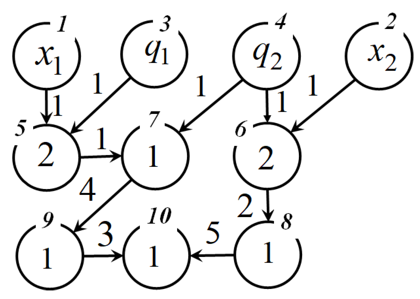
The network operator method encodes mathematical expressions in the form of directed graphs [5,27]. For coding, the method uses functions with one and two arguments. On the graph, functions with one argument are associated with the edges, functions with two arguments are associated with the nodes, and the arguments of the encoded mathematical expression are associated with the source nodes of the graph. Functions with two arguments must be commutative, associative, and have a unit element. An integer matrix of the network operator is used to store the code in the computer memory.

Let us consider an example of coding in the network operator method. Let a mathematical expression be given as

$$y=sin(cos(q_1{x}_1+q_2))+exp(-q_2{x}_2),$$

(38)

where $q_1$, $q_2$ are parameters, $x_1$, $x_2$ are variables. The parameters and the variables are arguments of the mathematical expression.

To encode a mathematical expression, it is sufficient to use the following sets of arguments and elementary functions

The set of arguments

$${\mathrm{F}}_0=\{x_1,x_2,q_1,q_2\}.$$

(39)

The set of function with one argument

$$\begin{array}{ccc}\hfill {\mathrm{F}}_1& =& \{f_{1,1}\left(z\right)=z,f_{1,2}\left(z\right)=-z,f_{1,3}\left(z\right)=sin\left(z\right),\hfill \\ \hfill & & f_{1,4}\left(z\right)=cos\left(z\right),f_{1,5}\left(z\right)=exp\left(z\right)\}.\hfill \end{array}$$

(40)

The set of function with two arguments

$${\mathrm{F}}_2=\{f_{2,1}(z_1,z_2)=z_1+z_2,f_{2,2}(z_1,z_2)=z_1{z}_2\}.$$

(41)

The graph of the network operator for (38) is given in Figure 1. In the source nodes of the graph, there are arguments of the mathematical expression. The remaining nodes contain indices of functions with two arguments. Next to the edges there are indices of functions with one argument. The indices correspond to the second index of elements in the sets of elementary functions (40) and (41). The nodes are enumerated according to topological sorting in their upper parts. The number of the node from which the edge exits is less than the number of the node where the edge enters. Such enumeration is always possible for graphs without loops, and it allows one to obtain an upper triangular matrix of the network operator. For nodes 8 and 9, the second argument is not specified. We use a unit element, zero for the addition function, as the second argument.

The network operator matrix for (38) is the following

$$\mathsf{\Psi }=\left[\begin{array}{cccccccccc}0& 0& 0& 0& 1& 0& 0& 0& 0& 0\\ 0& 0& 0& 0& 0& 1& 0& 0& 0& 0\\ 0& 0& 0& 0& 1& 0& 0& 0& 0& 0\\ 0& 0& 0& 0& 0& 1& 1& 0& 0& 0\\ 0& 0& 0& 0& 2& 0& 1& 0& 0& 0\\ 0& 0& 0& 0& 0& 2& 0& 2& 0& 0\\ 0& 0& 0& 0& 0& 0& 1& 0& 4& 0\\ 0& 0& 0& 0& 0& 0& 0& 1& 0& 5\\ 0& 0& 0& 0& 0& 0& 0& 0& 1& 3\\ 0& 0& 0& 0& 0& 0& 0& 0& 0& 1\end{array}\right].$$

(42)

The numbers of rows and columns in the network operator matrix correspond to the node number in the graph. Edges exiting the node are located in a row, edges entering a node are located in a column. The diagonal elements contain indices of functions with two arguments. The rest nonzero elements are the indices of functions with one argument.

Let us introduce small variations for the code of the network operator: 1—replacement of a nonzero off-diagonal element, 2—replacement of a nonzero diagonal element, 3—replacement of a zero off-diagonal element, 4—zeroing of an off-diagonal nonzero element. Small variation 4 is performed only if at least one off-diagonal nonzero element remains in the given row and in the given column.

To present a small variation use a vector of four components

$$\mathbf{w}={\left[w_1{w}_2{w}_3{w}_4\right]}^T,$$

(43)

where $w_1$ is an index of small variation, $w_2$ is an index of row, $w_3$ is an index of column, $w_4$ is a new value of element.

Suppose that we have a set of four vectors of variations

$$\begin{array}{c}{\mathbf{w}}^1={\left[1792\right]}^T,\\ {\mathbf{w}}^2={\left[4681\right]}^T,\\ {\mathbf{w}}^3={\left[2661\right]}^T,\\ {\mathbf{w}}^4={\left[3593\right]}^T.\end{array}$$

(44)

If we apply this set of variations to the network operator matrix (42), we obtain a new network operator matrix

$${\mathbf{w}}^4\circ {\mathbf{w}}^3\circ {\mathbf{w}}^2\circ {\mathbf{w}}^1\circ \mathsf{\Psi }=\left[\begin{array}{cccccccccc}0& 0& 0& 0& 1& 0& 0& 0& 0& 0\\ 0& 0& 0& 0& 0& 1& 0& 0& 0& 0\\ 0& 0& 0& 0& 1& 0& 0& 0& 0& 0\\ 0& 0& 0& 0& 0& 1& 1& 0& 0& 0\\ 0& 0& 0& 0& 2& 0& 1& 0& 3& 0\\ 0& 0& 0& 0& 0& 1& 0& 2& 0& 0\\ 0& 0& 0& 0& 0& 0& 1& 0& 2& 0\\ 0& 0& 0& 0& 0& 0& 0& 1& 0& 5\\ 0& 0& 0& 0& 0& 0& 0& 0& 1& 3\\ 0& 0& 0& 0& 0& 0& 0& 0& 0& 1\end{array}\right].$$

(45)

Note that the second variation ${\mathbf{w}}^2$ cannot be performed since, after this, there will be no nonzero nondiagonal elements left.

New network operator matrix (45) corresponds to the following mathematical expression

$$y=sin(-(q_1{x}_1+q_2)+sin\left(q_1{x}_1\right))+exp(-(q_2+x2)).$$

(46)

4.2. Variational Genetic Programming

The GP code for a mathematical expression is a computational tree. Arguments of a mathematical expression are located on the branches of the tree. The computational tree for the mathematical expression (38) is shown in Figure 2.

In GP computational tree functions are placed in the nodes. The functions from the sets (40) and (41) were used. The number of arguments in the leaves of the tree must match the number of times these arguments are used in the expression. For example, the parameter $q_2$ appears in a mathematical expression twice, so it appears twice in the leaves of the tree.

To store the computational tree in the computer memory a vector of two components is used

$${\mathbf{s}}_{GP}={\left[s_1{s}_2\right]}^T,$$

(47)

where $s_1$ is a number of function arguments, $s_2$ is the function index.

Arguments of a mathematical expression are represented as functions without arguments

$${\mathrm{F}}_0=\{f_{0,1}=x_1,f_{0,2}=x_2,f_{0,3}=q_1,f_{0,4}=q_2\}.$$

(48)

GP code for (38) is

$$\begin{array}{ccc}\hfill \mathrm{S}& =& ({\left[21\right]}^T,{\left[13\right]}^T,{\left[14\right]}^T,{\left[21\right]}^T,{\left[22\right]}^T,{\left[01\right]}^T,{\left[03\right]}^T,\hfill \\ \hfill & & {\left[04\right]}^T,{\left[15\right]}^T,{\left[12\right]}^T,{\left[22\right]}^T,{\left[02\right]}^T,{\left[04\right]}^T).\hfill \end{array}$$

(49)

Let us define small variations for GP: 1—change of the second component of the function code vector, while the value of the second component indicates the index of the element from the set given by the first component; 2—removal of the vector of the function code with one argument; 3—insertion of a function code vector with one argument; 4—increasing the value of the first component of the function vector code, while the vector of the argument code is inserted after the code of the function; 5—decreasing the value of the first component of the function vector code by one, while deleting the first argument code encountered after the variable code. If a contradiction arises when performing a variation, then the small variation is not performed.

To code small variation for GP we use a vector of variation of tree components

$$\mathbf{w}={\left[w_1{w}_2{w}_3\right]}^T,$$

(50)

where $w_1$ is a type of variation, $w_1\in \{1,\dots ,5\}$, $w_2$ is an index of variable element, $w_3$ is a value of new element.

Suppose that for a GP code (49) of expression (38) the following variations are defined

$$\begin{array}{ccc}\hfill {\mathbf{w}}^1& =& {\left[142\right]}^T,\hfill \\ \hfill {\mathbf{w}}^2& =& {\left[231\right]}^T,\hfill \\ \hfill {\mathbf{w}}^3& =& {\left[491\right]}^T\hfill \\ \hfill {\mathbf{w}}^4& =& {\left[354\right]}^T\hfill \\ \hfill {\mathbf{w}}^5& =& {\left[5121\right]}^T\hfill \end{array}$$

(51)

Perform small variations for code (49)

$$\begin{array}{ccc}\hfill {\mathbf{w}}^1\circ \mathrm{S}& =& ({\left[21\right]}^T,{\left[13\right]}^T,{\left[14\right]}^T,{\left[22\right]}^T,{\left[22\right]}^T,{\left[01\right]}^T,{\left[03\right]}^T,\hfill \\ \hfill & & {\left[04\right]}^T,{\left[13\right]}^T,{\left[12\right]}^T,{\left[22\right]}^T,{\left[02\right]}^T,{\left[04\right]}^T),\hfill \end{array}$$

(52)

$$\begin{array}{ccc}\hfill {\mathbf{w}}^2\circ {\mathbf{w}}^1\circ \mathrm{S}& =& ({\left[21\right]}^T,{\left[13\right]}^T,{\left[22\right]}^T,{\left[22\right]}^T,{\left[01\right]}^T,{\left[03\right]}^T,\hfill \\ \hfill & & {\left[04\right]}^T,{\left[13\right]}^T,{\left[12\right]}^T,{\left[22\right]}^T,{\left[02\right]}^T,{\left[04\right]}^T),\hfill \end{array}$$

(53)

$$\begin{array}{ccc}\hfill {\mathbf{w}}^3\circ {\mathbf{w}}^2\circ {\mathbf{w}}^1\circ \mathrm{S}& =& ({\left[21\right]}^T,{\left[13\right]}^T,{\left[22\right]}^T,{\left[22\right]}^T,{\left[01\right]}^T,\hfill \\ \hfill & & {\left[03\right]}^T,{\left[04\right]}^T,{\left[13\right]}^T,{\left[22\right]}^T,{\left[01\right]}^T,\hfill \\ \hfill & & {\left[22\right]}^T,{\left[02\right]}^T,{\left[04\right]}^T),\hfill \end{array}$$

(54)

$$\begin{array}{ccc}\hfill {\mathbf{w}}^4\circ {\mathbf{w}}^3\circ {\mathbf{w}}^2\circ {\mathbf{w}}^1\circ \mathrm{S}& =& ({\left[21\right]}^T,{\left[13\right]}^T,{\left[22\right]}^T,{\left[22\right]}^T,{\left[14\right]}^T,\hfill \\ \hfill & & {\left[01\right]}^T,{\left[03\right]}^T,{\left[04\right]}^T,{\left[13\right]}^T,{\left[22\right]}^T,\hfill \\ \hfill & & {\left[01\right]}^T,{\left[22\right]}^T,{\left[02\right]}^T,{\left[04\right]}^T),\hfill \end{array}$$

(55)

$$\begin{array}{ccc}\hfill {\mathbf{w}}^5\circ {\mathbf{w}}^4\circ {\mathbf{w}}^3\circ {\mathbf{w}}^2\circ {\mathbf{w}}^1\circ \mathrm{S}& =& ({\left[21\right]}^T,{\left[13\right]}^T,{\left[22\right]}^T,{\left[22\right]}^T,{\left[14\right]}^T,\hfill \\ \hfill & & {\left[01\right]}^T,{\left[03\right]}^T,{\left[04\right]}^T,{\left[13\right]}^T,{\left[22\right]}^T,\hfill \\ \hfill & & {\left[01\right]}^T,{\left[12\right]}^T,{\left[04\right]}^T).\hfill \end{array}$$

(56)

As a result of small variations (51) for code (49), we obtain a code (56) of expression

$$y=sin(q_1{q}_{2}cos\left(x_1\right))+sin(-x_1{q}_2).$$

(57)

4.3. Variational Cartesian Genetic Programming

Cartesian genetic programming (CGP) does not use graphs to present codes of expressions. All elementary functions are combined into one set. The number of function arguments is determined by its index. A mathematical expression is coded as a sequence of calls of elementary functions. Each function call is coded by an integer vector. The first element of the vector is the function index, the remaining elements are the indices of elements from the set of arguments. The result of the calculation of the function call is immediately added to the set of arguments so that it can be used in subsequent calls.

Consider an example of coding mathematical expression (38) by CGP. We will use the set of arguments (39), combine all functions from (40) and (41) into one set, and exclude identity function $f_{1,1}\left(z\right)=z$

$$\begin{array}{ccc}\hfill \mathrm{F}& =& \{f_1\left(z\right)=-z,f_2\left(z\right)=sin\left(z\right),f_3\left(z\right)=cos\left(z\right),\hfill \\ \hfill & & f_4\left(z\right)=exp\left(z\right),f_5(z_1,z_2)=z_1+z_2,f_6(z_1,z_2)=z_1{z}_2\left)\right\}.\hfill \end{array}$$

(58)

Since in (58) there are only functions with one and two arguments, it is sufficient to use a vector of three elements to encode a function call. For the function with one argument, the third element is not used.

The CGP for a mathematical expression (38) is as follows

$$\mathrm{S}=\left(\left[\begin{array}{c}6\\ 3\\ 1\end{array}\right],\left[\begin{array}{c}5\\ 5\\ 4\end{array}\right],\left[\begin{array}{c}3\\ 6\\ 1\end{array}\right],\left[\begin{array}{c}2\\ 7\\ 2\end{array}\right],\left[\begin{array}{c}6\\ 4\\ 2\end{array}\right],\left[\begin{array}{c}1\\ 9\\ 3\end{array}\right],\left[\begin{array}{c}4\\ 10\\ 4\end{array}\right],\left[\begin{array}{c}5\\ 8\\ 11\end{array}\right]\right).$$

(59)

Small variation of code in CGP is a change of one element of the code [28]. To present a small variation, it is enough to use an integer vector of three elements

$$\mathbf{w}={\left[w_1{w}_2{w}_3\right]}^T,$$

(60)

where $w_1$ is an index of column in the code, $w_2$ is an index of row in the column $w_1$, and $w_3$ is a new value of the element.

If we vary the first element of the vector of an elementary function, then its new value is determined by the index of the element from the set of elementary functions (58). If we vary some other element, then its value must be less than the sum of the number of elements in the set of arguments (39) and the index $w_1$ of the varied call vector.

Let us define some variations of the CGP code of (59).

$$\begin{array}{ccc}\hfill {\mathbf{w}}^1& =& {\left[213\right]}^T,\hfill \\ \hfill {\mathbf{w}}^2& =& {\left[325\right]}^T,\hfill \\ \hfill {\mathbf{w}}^3& =& {\left[628\right]}^T,\hfill \\ \hfill {\mathbf{w}}^3& =& {\left[616\right]}^T.\hfill \end{array}$$

(61)

Having performed small variations (61), we obtain the following CGP code

$${\mathbf{w}}^4\circ {\mathbf{w}}^3\circ {\mathbf{w}}^2\circ {\mathbf{w}}^1\circ \mathrm{S}=\left(\left[\begin{array}{c}6\\ 3\\ 1\end{array}\right],\left[\begin{array}{c}3\\ 5\\ 4\end{array}\right],\left[\begin{array}{c}3\\ 5\\ 1\end{array}\right],\left[\begin{array}{c}2\\ 7\\ 2\end{array}\right],\left[\begin{array}{c}6\\ 4\\ 2\end{array}\right],\left[\begin{array}{c}6\\ 8\\ 3\end{array}\right],\left[\begin{array}{c}4\\ 10\\ 4\end{array}\right],\left[\begin{array}{c}5\\ 8\\ 11\end{array}\right]\right).$$

(62)

that corresponds to mathematical expression

$$y=exp(q_{1}sin(cos\left(q_1{x}_1\right)))+sin(cos\left(q_1{x}_1\right)).$$

(63)

The disadvantage of CGP is that some calls of function in the final mathematical expression may not be used.

4.4. Variational Complete Binary Genetic Programming

Complete binary genetic programming (CBGP) encodes mathematical expressions as complete binary trees. For this structure, only functions with one or two arguments are used. Functions with two arguments are associated with tree nodes, functions with one argument are are associated with tree branches. Arguments of mathematical expressions and unit elements for functions with two arguments are placed on the leaves of the tree. Since the tree is complete, the number of elements at each level is known. There is no need to specify the number of arguments for the function when writing code to store it in computer memory. The quantity of arguments is determined by the position of the function in the code. Unit elements for functions with two arguments are added to the set of arguments.

To encode a mathematical expression (38) by CBGP, we use sets of elementary functions with one and two arguments (40) and (41). We add unit elements for functions with two arguments in the set of arguments (39), i.e. zero for addition and one for multiplication

$${\mathrm{F}}_0=(f_1=x_1,f_2=x_2,f_3=q_1,f_4=q_2,f_5=0,f_6=1).$$

(64)

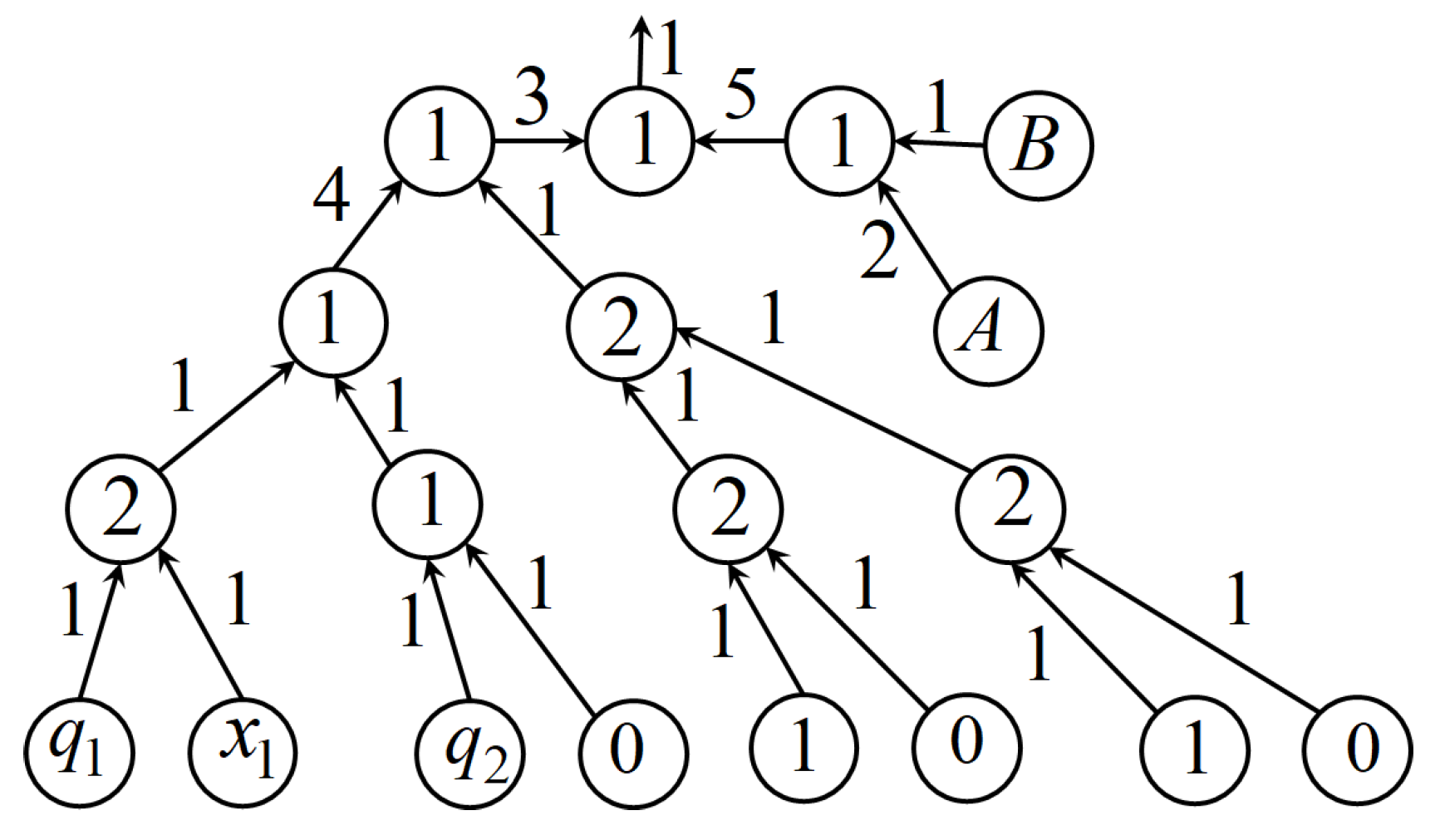
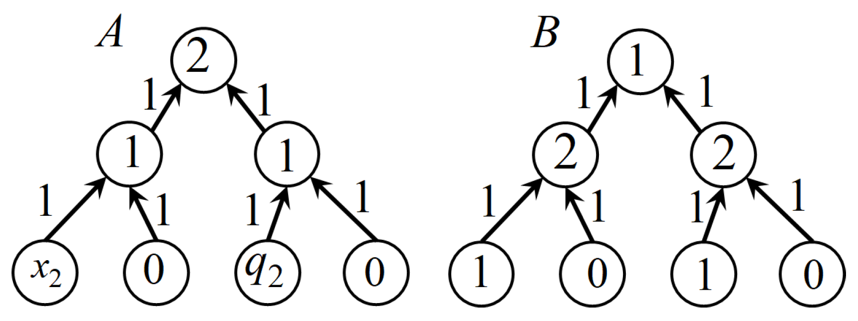
A CBGP computational tree for mathematical expression (38) is given in Figure 3 and Figure 4.

CBGP code is an ordered set of function indices from a tree, written sequentially from left to right. At the last level, the indices of arguments from the set (64) are indicated.

The CBGP code for mathematical expression (38) is

$$\begin{array}{ccc}\hfill \mathrm{S}& =& (1,1,\hfill \\ \hfill & & 3,5,1,1,\hfill \\ \hfill & & 4,1,2,1,1,2,2,1,\hfill \\ \hfill & & 1,1,1,1,1,1,1,1,2,1,2,2,1,1,2,2,\hfill \\ \hfill & & 1,1,1,1,1,1,1,1,1,1,1,1,1,1,1,1,3,1,4,5,6,5,6,5,2,5,4,5,6,5,6,5).\hfill \end{array}$$

(65)

Here, for convenience, the CBGP code is presented on different lines according to the levels of the tree. Each level k contains $2^k$ number of functions with one argument and the same number of functions with two arguments. Altogether, there are $2^{k+1}$ elements at the level k. The total number of elements L in the CBGP code for a binary tree with K levels is calculated as

$$L=\sum _{k=0}^K{2}^{k+1}=2^1+2^2+\dots +2^{K+1}=2^{K+2}-2.$$

(66)

In the considered example, we have $K=4$ levels and thus $2^{4+2}-2=62$ elements.

To determine whether element $f_{s_{\alpha }}$, where $\alpha$ is an index of element in the code, belongs to one of the sets ${\mathrm{F}}_0$, ${\mathrm{F}}_1$, or ${\mathrm{F}}_2$, we use the following relations

$$f_{s_{\alpha }}\in \left\{\begin{array}{c}{\mathrm{F}}_0,\mathrm{if}{2}^{k+2}-2^k⩽\alpha ⩽2^{k+2}-2\mathrm{and}k=K\hfill \\ {\mathrm{F}}_1,\mathrm{if}{2}^{k+1}-1⩽\alpha ⩽2^{k+2}-2^k-2\hfill \\ {\mathrm{F}}_2,\mathrm{if}{2}^{k+2}-2^k⩽\alpha ⩽2^{k+2}-2\mathrm{and}k<K\hfill \end{array}\right.,$$

(67)

where k is the smallest number, that satisfies inequality

$$\alpha ⩽2^{k+2}-2.$$

(68)

To present a small variation of CBGP code, let us use a vector of two elements

$$\mathbf{w}={\left[w_1{w}_2\right]}^T,$$

(69)

where $w_1$ is an index of element position and $w_2$ is a new value of element.

Consider an example of small variations of CBGP code (65) that describes the mathematical expression (38)

$$\begin{array}{ccc}\hfill {\mathbf{w}}^1& =& {\left[121\right]}^T,\hfill \\ \hfill {\mathbf{w}}^2& =& \left[553\right]\hfill \\ \hfill {\mathbf{w}}^3& =& {\left[75\right]}^T\hfill \\ \hfill {\mathbf{w}}^4& =& \left[501\right]\hfill \end{array}.$$

(70)

Having performed variations (70), we obtain a new CBGP code

$$\begin{array}{ccc}\hfill \mathrm{S}& =& (1,1,\hfill \\ \hfill & & 3,5,1,1,\hfill \\ \hfill & & 5,1,2,1,1,1,2,1,\hfill \\ \hfill & & 1,1,1,1,1,1,1,1,2,1,2,2,1,1,2,2,\hfill \\ \hfill & & 1,1,1,1,1,1,1,1,1,1,1,1,1,1,1,1,3,1,4,1,6,5,6,5,3,5,4,5,6,5,6,5).\hfill \end{array}$$

(71)

This code presents a new mathematical expression

$$y=sin(exp(q_1{x}_1+q_2+x_1))+exp(-(q_1+q_2)).$$

(72)

5. Computational Experiments

5.1. Case 1. Control Synthesis for Mobile Robot

As an example, let us consider the application of the variational symbolic regression method for control synthesis of a mobile robot. In the problem, it is necessary to find a mathematical expression for the control function that transfers the object from the set of initial conditions to the terminal one with the optimal value of the quality criterion.

The mathematical model [29] of control object is

$$\begin{array}{ccc}\hfill {\dot{x}}_1& =& 0.5(u_1+u_2)cos\left(x_3\right),\hfill \\ \hfill {\dot{x}}_2& =& 0.5(u_1+u_2)sin\left(x_3\right),\hfill \\ \hfill {\dot{x}}_3& =& 0.5(u_1-u_2),\hfill \end{array}$$

(73)

where $\mathbf{x}={\left[x_1{x}_2{x}_3\right]}^T$ is a state vector, $\mathbf{u}={\left[u_1{u}_2\right]}^T$ is a control vector.

The control is constrained

$$u^{-}=-10⩽u_i⩽10=u^{+},i=1,2.$$

(74)

The initial condition is a set of 30 states

$$\begin{array}{ccc}\hfill {\mathrm{X}}_0& =& \{{\mathbf{x}}^{0,1}={[22.55\pi /12]}^T,{\mathbf{x}}^{0,2}={[12.55\pi /12]}^T,{\mathbf{x}}^{0,3}={[02.55\pi /12]}^T,\hfill \\ \hfill & & {\mathbf{x}}^{0,4}={[-12.55\pi /12]}^T,{\mathbf{x}}^{0,5}={[-22.55\pi /12]}^T,\hfill \\ \hfill & & {\mathbf{x}}^{0,6}={[2-2.55\pi /12]}^T,{\mathbf{x}}^{0,7}={[1-2.55\pi /12]}^T,\hfill \\ \hfill & & {\mathbf{x}}^{0,8}={[0-2.55\pi /12]}^T,{\mathbf{x}}^{0,9}={[-1-2.55\pi /12]}^T,\hfill \\ \hfill & & {\mathbf{x}}^{0,10}={[-2-2.55\pi /12]}^T,{\mathbf{x}}^{0,11}={\left[22.50\right]}^T,{\mathbf{x}}^{0,12}={\left[12.50\right]}^T,\hfill \\ \hfill & & {\mathbf{x}}^{0,13}={\left[02.50\right]}^T,{\mathbf{x}}^{0,14}={[-12.50]}^T,{\mathbf{x}}^{0,15}={[-22.50]}^T,\hfill \\ \hfill & & {\mathbf{x}}^{0,16}={[2-2.50]}^T,{\mathbf{x}}^{0,17}={[1-2.50]}^T,{\mathbf{x}}^{0,18}={[0-2.50]}^T,\hfill \\ \hfill & & {\mathbf{x}}^{0,19}={[-1-2.50]}^T,{\mathbf{x}}^{0,20}={[-2-2.50]}^T,\hfill \\ \hfill & & {\mathbf{x}}^{0,21}={[22.5-5\pi /12]}^T,{\mathbf{x}}^{0,22}={[12.5-5\pi /12]}^T,\hfill \\ \hfill & & {\mathbf{x}}^{0,23}={[02.5-5\pi /12]}^T,{\mathbf{x}}^{0,24}={[-12.5-5\pi /12]}^T,\hfill \\ \hfill & & {\mathbf{x}}^{0,25}={[-22.5-5\pi /12]}^T,{\mathbf{x}}^{0,26}={[2-2.5-5\pi /12]}^T,\hfill \\ \hfill & & {\mathbf{x}}^{0,27}={[1-2.5-5\pi /12]}^T,{\mathbf{x}}^{0,28}={[0-2.5-5\pi /12]}^T,\hfill \\ \hfill & & {\mathbf{x}}^{0,29}={[-1-2.5-5\pi /12]}^T,{\mathbf{x}}^{0,30}={[-2-2.5-5\pi /12]}^T\}.\hfill \end{array}$$

(75)

The terminal condition is

$${\mathbf{x}}^f={\left[000\right]}^T.$$

(76)

It is necessary to find a control as a function of state coordinates

$$u_i=h_i(x_1,x_2,x_3),u^{-}⩽h_i(x_1,x_2,x_3)⩽u^{+},i=1,2,$$

(77)

to minimize the functional

$$J=\sum _{k=1}^{30}\left(t_{f,k}+\sqrt{\sum _{i=1}^3{x}_i^2(t_{f,k},{\mathbf{x}}^{0,k})}\right),$$

(78)

where

$$t_{f,k}=\left\{\begin{array}{c}t,\mathrm{if}\sqrt{{\sum }_{i=1}^3{x}_i^2(t,{\mathbf{x}}^{0,k})}<\epsilon \hfill \\ t^{+},\mathrm{otherwise}\hfill \end{array}\right.,$$

(79)

$\epsilon =0.01$, $t^{+}=1.5$ s, $x_i(t,{\mathbf{x}}^{0,k})$ is a partial solution of ODE system (73) with control (77) for initial state ${\mathbf{x}}^{0,k}$, $k\in \{1,\dots ,30\}$.

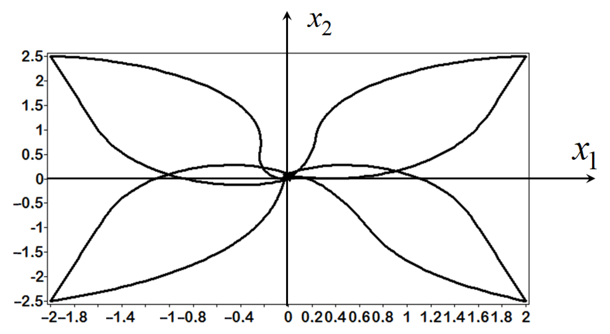
To solve the problem, we used variational CGP and obtained the following control function

$$h_i(x_1,x_2,x_3)=\left\{\begin{array}{c}{u}^{-},\mathrm{if}{\tilde{u}}_i<u^{-}\hfill \\ u^{+},\mathrm{if}{\tilde{u}}_i>u^{+}\hfill \\ {\tilde{u}}_i,\mathrm{otherwise}\hfill \end{array}\right.,i=1,2,$$

(80)

where

$$\begin{array}{ccc}\hfill {\tilde{u}}_1& =& \mathrm{sgn}(arctan(q_2{x}_2/\left(q_3{x}_1\right)+1/x_1))(exp(q_{3}arctan(q_2{x}_2/\left(q_3{x}_1\right)+\hfill \\ \hfill & & 1/x_1\left)\right)-1)-3q_3{x}_1-x_3\hfill \\ \hfill {\tilde{u}}_2& =& \left(\right(-q_3{x}_1-x_2-\mathrm{sgn}(q_2{x}_2/\left(q_3{x}_1\right)+1/x_1)\times \hfill \\ \hfill & & (exp(q_{3}arctan(q_2{x}_2/\left(q_3{x}_1\right)+1/x_1))-1){{)}^3+1+q_1)}^3\hfill \end{array}$$

(81)

$q_1=2.74121$, $q_2=1.82129$, $q_3=3.88281$. The value of quality criterion (78) for the solution is $J=34.6372$.

Trajectories of mobile robot from different initial states to terminal one on plane are presented on Figure 5. To solve the problem, the system (73) was integrated 2,386,440 times. The calculations were performed on Intel Core i7, 2.8 GHz. The computational time was approx. 15 min.

It should be noted here that CGP without applying the principle of small variations of the basic solution did not cope with the solution of the problem and could not find a single acceptable solution with the same search parameters.

5.2. Case 2. Knapsack Problem

Consider a classic NP-hard knapsack problem. We need to choose, among a number of objects, some set of objects that satisfy certain criteria. Vector of small variations consists of two elements: 1—index of element in the set of objects; 2—a new value.

Suppose that the capacity of knapsack is C. The set of objects with some weights is

$$\mathrm{X}=(x_1,\dots ,x_K),x^{-}⩽x_i⩽x^{+},i=\overline{1,K},$$

(82)

where $x^{-}$ and $x^{+}$ are low and upper values of objects, K is a number of objects.

Each possible solution is

$$\mathbf{y}=[y_1\dots y_K],y_i\in \{0,1\},i=\overline{1,K}.$$

(83)

It is necessary to find a vector $\mathbf{y}$ to minimize the following quality criterion

$$F\left(\mathbf{y}\right)=|C^{*}-\sum _{i=1}^K{y}_i{x}_i|\to \min ,$$

(84)

so that the weight of objects would be as close to the capacity of knapsack as possible.

Consider the following example. We have a $K=100$ objects that have real values (suppose weights, kg) from 0 to 10. The capacity of the knapsack is 100 kg. We need to choose the objects so that their total weight is close to the capacity. In general case there are different types of constraints, on weight, volume, costs, etc.

To solve this problem, we applied VarGA. The parameters of algorithm are given in

Table 1. Parameters of VarGA for the knapsack problem.

Parameter	Value
Number of solutions in generation	1024
Number of generations	128
Number of crossovers	128
Depth of variation	8
Number of generations between epochs	8
Probability of mutation	0.75

.

The set of objects is

$$\begin{array}{ccc}\hfill \mathrm{X}& =& \{x_1=1.198973,x_2=8.195864,x_3=0.149163,x_4=0.600499,\hfill \\ \hfill & & x_5=1.868563,x_6=1.134450,x_7=2.940746,x_8=3.005569,\hfill \\ \hfill & & x_9=0.235667,x_{10}=6.92442,x_{11}=9.862742,x_{12}=9.013933,\hfill \\ \hfill & & x_{13}=1.685997,x_{14}=4.716708,x_{15}=1.805467,x_{16}=3.955157,\hfill \\ \hfill & & x_{17}=3.605431,x_{18}=3.456106,x_{19}=4.063158,x_{20}=8.704509,\hfill \\ \hfill & & x_{21}=1.290323,x_{22}=7.570359,x_{23}=0.605452,x_{24}=5.840240,\hfill \\ \hfill & & x_{25}=7.466071,x_{26}=7.852390,x_{27}=0.020214,x_{28}=4.903944,\hfill \\ \hfill & & x_{29}=7.782723,x_{30}=8.912633,x_{31}=8.311701,x_{32}=4.629041,\hfill \\ \hfill & & x_{33}=9.999174,x_{34}=0.188699,x_{35}=2.837382,x_{36}=6.866526,\hfill \\ \hfill & & x_{37}=3.853656,x_{38}=9.422472,x_{39}=7.059892,x_{40}=5.666469,\hfill \\ \hfill & & x_{41}=7.686985,x_{42}=6.470105,x_{43}=3.892209,x_{44}=0.501044,\hfill \\ \hfill & & x_{45}=3.471120,x_{46}=3.024267,x_{47}=1.730138,x_{48}=8.358248,\hfill \\ \hfill & & x_{49}=0.700096,x_{50}=8.905066,x_{51}=6.966928,x_{52}=3.520369,\hfill \\ \hfill & & x_{53}=3.283775,x_{54}=9.267853,x_{55}=0.620899,x_{56}=7.016356,\hfill \\ \hfill & & x_{57}=9.203328,x_{58}=4.219690,x_{59}=1.891819,x_{60}=3.921507,\hfill \\ \hfill & & x_{61}=4.049162,x_{62}=5.061787,x_{63}=9.480431,x_{64}=6.256851,\hfill \\ \hfill & & x_{65}=0.661214,x_{66}=5.630264,x_{67}=9.411684,x_{68}=5.275044,\hfill \\ \hfill & & x_{69}=4.325184,x_{70}=1.710065,x_{71}=2.823965,x_{72}=1.055504,\hfill \\ \hfill & & x_{73}=8.029722,x_{74}=5.355668,x_{75}=1.084831,x_{76}=9.075759,\hfill \\ \hfill & & x_{77}=6.102632,x_{78}=8.207962,x_{79}=1.945653,x_{80}=0.996382,\hfill \\ \hfill & & x_{81}=7.408127,x_{82}=5.727311,x_{83}=2.674080,x_{84}=4.547363,\hfill \\ \hfill & & x_{85}=7.281093,x_{86}=6.022923,x_{87}=3.066631,x_{88}=5.206564,\hfill \\ \hfill & & x_{89}=2.919562,x_{90}=0.500339,x_{91}=0.182961,x_{92}=7.070480,\hfill \\ \hfill & & x_{93}=9.648925,x_{94}=8.176261,x_{95}=6.963208,x_{96}=3.829286,\hfill \\ \hfill & & x_{97}=3.794559,x_{98}=6.652624,x_{99}=4.438315,x_{100}=0.459797\}.\hfill \end{array}$$

(85)

As a result, we obtained the following solution

$$\begin{array}{ccc}\hfill y_i& =& 1,\hfill \\ \hfill i& =& 1,4,5,6,11,14,15,16,21,23,27,28,29,31,32,\hfill \\ \hfill & & 43,44,46,47,48,51,59,65,69,78,90,91,92.\hfill \end{array}$$

(86)

The objective function for this solution is $F\left(\mathbf{y}\right)=0.00125$,

$$\sum _{i=1}^{100}{y}_i{x}_i=99.998749.$$

(87)

6. Results

Symbolic regression methods are currently used to solve complex optimization problems in non-numeric spaces. To expand the area of their application and, in particular, to simplify the execution of the operations of the genetic algorithm, a universal approach was developed based on the principle of small variations of the basic solution.

The main definitions, the distance between the codes, and the neighborhood of the code, including the concept of the inheritance property, were given. A proof of the theorem was presented for solving an optimization problem on a non-numerical space, and provided that the value of the functional is uniformly distributed over a certain interval, the use of symbolic regression methods with the inheritance property for search of optimal solution on a non-numerical space is more efficient than the random search.

Examples of constructing small variations of the basic solution for various methods of symbolic regression were given. It is proposed that the methods which use the principle of small variations be called variational. An example of solving the synthesis problem was given, in which it was necessary to find one control function to ensure the transfer of an object from 30 initial conditions to one terminal point according to the criterion of speed and accuracy. The problem was solved by the variational Cartesian genetic programming. In addition, the classical NP-hard knapsack problem for 100 objects was solved using a variational genetic algorithm.

The results presented in the article have both fundamental and practical importance.

7. Discussion

The principle of small variations of basic solution is considered as a universal approach to solving problems using symbolic regression methods. In the future, it is proposed to expand the area of its application for solving other optimization problems on a non-numerical space.

The set of types of elementary variations can be expanded by introducing new variations: inserting a code element at a certain position with a shift of the rest of the code to the right, deleting a code element with a shift to the left, exchanging code elements, etc. The depth of variations, that is, the number of small variations applied to the basic solution for obtaining a new code, affects the computational time to find the optimal solution and may vary. The study of the effectiveness of using various types of small variations and their depth are tasks to be solved.

8. Patents

Certificate of software registration No. 2020619911 Sofronova, E.A., Diveev, A.I., “Program for simulation and optimal control of traffic lights by variational genetic algorithm”, 25 August 2020.

Certificate of software registration No. 2021611714 Diveev, A.I. Shmalko, E.Yu. Konstantinov, S.V., “Synthesis of a multidimensional control function from the object state based on the approximation of optimal directories by the method of the network operator”, 3 February 2021.

Certificate of software registration No. 2021611899 Diveev, A.I. Shmalko, E.Yu., “Synthesis of a stabilization system based on variational Cartesian genetic programming”, 8 February 2021.

References

Koza, J.R. Genetic Programming; MIT Press: Cambridge, MA, USA, 1992. [Google Scholar]
O’Neil, M.; Ryan, C. Grammatical Evolution. IEEE Trans. Evol. Comput.2001, 4, 349–358. [Google Scholar] [CrossRef]
Miller, J.; Thomson, P. Cartesian Genetic Programming. In Genetic Programming. EuroGP; Poli, R., Banzhaf, W., Langdon, W.B., Miller, J., Nordin, P., Fogarty, T.C., Eds.; Lecture Notes in Computer Science Series; Springer: Berlin/Heidelberg, Germany, 2000; Volume 1802. [Google Scholar]
Zelinka, I.; Oplatkova, Z.; Nolle, L. Analytic Programming—Symbolic Regression by Means of Arbitrary Evolutionary Algorithms. Int. J. Smart Secur. Technol. (IJSST)2005, 9, 44–56. [Google Scholar]
Diveev, A.I.; Sofronova, E.A. Numerical method of network operator for multiobjective synthesis of optimal control system. In Proceedings of the Seventh International Conference on Control and Automation (ICCA’09), Christchurch, New Zealand, 9–11 December 2009; pp. 701–708. [Google Scholar]
Diveev, A.I.; Sofronova, E.A. Automation of Synthesized Optimal Control Problem Solution for Mobile Robot by Genetic Programming. In Intelligent Systems and Applications, Proceedings of the 2019 Intelligent Systems Conference (Intellisys), London, UK, 5–6 September 2019; Be, Y., Bhatia, R., Kapoor, S., Eds.; Advances in Intelligent Systems and Computing Series; Springer: Cham, Switzerland, 2019; Volume 2, pp. 1054–1072. [Google Scholar]
Arnaldo, I.; O’Reilly, U.-M.; Veeramachaneni, K. Building predictive models via feature synthesis. In Proceedings of the 2015 Annual Conference on Genetic and Evolutionary Computation, Madrid, Spain, 11–15 July 2015; pp. 983–990. [Google Scholar]
Brunton, S.L.; Proctor, J.L.; Kutz, J.N. Discovering govering equations from data by sparse identification of nonlinear dynamical systems. Proc. Natl. Acad. Sci. USA2016, 113, 3932–3937. [Google Scholar] [CrossRef] [PubMed]
Quade, M.; Abel, M.; Nathanutz, J.; Brunton, S.L. Sparse identification of nonlinear dynamics for rapid model recovery. Chaos2018, 28, 063116. [Google Scholar] [CrossRef] [PubMed]
McRee, R.K. Symbolic regression using nearest neighbor indexing. In Proceedings of the 12th Annual Conference Companion on Genetic and Evolutionary Comutation, GECCO’10, Portland, OR, USA, 7–11 July 2010; pp. 1983–1990. [Google Scholar]
Kong, W.; Liaw, C.; Mehta, A.; Sivakumar, D. A new dog learns old tricks: RL finds classic optimization algorithms. In Proceedings of the International Conference on Learning Representations, New Orleans, LA, USA, 6–9 May 2019; pp. 1–25. [Google Scholar]
Nikolaev, N.; Iba, H. Inductive Genetic Programming of Polynomial Learning Networks. In 2000 IEEE Symposium on Combinations of Evolutionary Computation and Neural Networks, Proceedings of the First IEEE Symposium of Combinations of Evolutionary Computation and Neural Networks, ECNN-2000, San Antonio, TX, USA, 11–13 May 2000; Yao, X., Ed.; IEEE Press: Piscataway, NJ, USA, 2000; pp. 158–167. [Google Scholar]
Schmidt, M.; Lipson, H. Distilling free-form natural laws from experimental data. Science2009, 324, 81–85. [Google Scholar] [CrossRef] [PubMed]
Diveev, A.; Kazaryan, D.; Sofronova, E. Symbolic regression methods for control system synthesis. In Proceedings of the 22nd Mediterranean Conference on Control and Automation, Palermo, Italy, 16–19 June 2014; pp. 587–592. [Google Scholar]
Eiben, A.E. Grand challenges for evolutionary robotics. Front. Robot. AI2014, 4, 1–2. [Google Scholar] [CrossRef]
Smetka, T.; Homoliak, I.; Hanacek, P. On the Application of Symbolic Regression and Genetic Programming for Cryptanalysis of Symmetric Encryption Algorithm. In Proceedings of the International Carnahan Conference on Security Technology (ICCST 2016), Orlando, FL, USA, 24–27 October 2016; pp. 1–8. [Google Scholar]
Linden, D.S. Optimizing signal strength in-situ using an evolvable antenna system. In Proceedings of the 2002 NASA/DoD Conference on Evolvable Hardware, Alexandria, VA, USA, 15–18 July 2002; pp. 147–151. [Google Scholar]
McAleer, S.; Agostinelli, F.; Shmakov, A.; Baldi, P. Solving the Rubik’s Cube with Approximate Policy Iteration. In Proceedings of the International Conference on Learning Representations, New Orleans, LA, USA, 6–9 May 2019; pp. 1–13. [Google Scholar]
Kim, S.; Lu, P.; Mukherjee, S.; Gilbert, M.; Jing, L.; Ceperic, V.; Soljacic, M. Integration of Neural Network-Based Symbolic Regression in Deep Learning for Scientific Discovery. arXiv2019, arXiv:1912.04825. [Google Scholar] [CrossRef] [PubMed]
Diveyev, A.I.; Sofronova, E.A. Application of network operator method for synthesis of optimal structure and parameters of automatic control system. IFAC Proc. Vol.2008, 41, 6106–6113. [Google Scholar] [CrossRef]
Cranmer, M.; Sanchez-Gonzalez, A.; Battaglia, P.; Xu, R.; Cranmer, K.; Spergel, D.; Ho, S. Discovering Symbolic Models from Deep Learning with Inductive Biases. arXiv2006, arXiv:2006.11287. [Google Scholar]
Udrescu, S.M.; Tegmark, M. Al Feynman: A physics-inspired method for symbolic regression. Sci. Adv.2020, 6, eaay2631. [Google Scholar] [CrossRef]
Diveev, A. Small Variations of Basic Solution Method for Non-numerical Optimization. IFAC-PapersOnLine2015, 48, 028–033. [Google Scholar] [CrossRef]
Levenshtein, V.I. Binary codes capable of correcting deletions, insertions, and reversals. Dokl. Akad. Nauk SSSR1965, 163, 845–848. [Google Scholar]
Holland, J.H. Adaptation in Natural and Artificial Systems, 2nd ed.; MIT Press: Cambridge, MA, USA, 1992; p. 232. [Google Scholar]
Diveev, A.I. A Numerical Method for Network Operator for Synthesis of a Control System with Uncertain Initial Values. J. Comput. Syst. Sci. Int.2012, 51, 228–243. [Google Scholar] [CrossRef]
Diveev, A.I. Cartesian Genetic Programming for Synthesis of Optimal Control System. In Proceedings of the Future Technologies Conference (FTC) 2020, Virtual Event, San Francisco, CA, USA, 5–6 November 2020; Arai, K., Kapoor, S., Bhatia, R., Eds.; Springer Nature: Cham, Switzerland, 2021; Volume 2, pp. 205–222. [Google Scholar]
Šuster, P.; Jadlovská, A. Tracking Trajectory of the Mobile Robot Khepera II Using Approaches of Artificial Intelligence. Acta Electrotech. Inform.2011, 11, 38–43. [Google Scholar] [CrossRef]
Figure 1.
The network operator graph for mathematical expression (38).
Figure 2.
GP computational tree for mathematical expression (38).
Figure 3.
CBGP computational tree for mathematical expression (38).
Figure 4.
CBGP computational tree for mathematical expression (38) (continued).
Figure 5.
Trajectories of mobile robot from eight initial states.