A Scheduling Algorithm for Multi-Workshop Production Based on BOM and Process Route

Abstract

For the scheduling problem of complex products in multi-workshop production, this paper studied the BOM (Bill of Materials) structure of complex products and the characteristics of the process route and developed the construction method of a multi-level process network diagram. Based on this, a comprehensive mathematical model for scheduling on multi-workshop production was proposed. An improved particle swarm algorithm (PSO) was proposed to solve the problem. By constructing the network subgraph, the invalid search path of the algorithm was avoided, and the efficiency of the algorithm was improved. In addition, for the scheduling problem with product time constraints, this paper presented a path search rescheduling strategy to ensure that the algorithm could obtain an effective search path. Finally, the model and algorithm were verified through a case study. This paper optimized the parameters of the algorithm by different tests and obtained the optimal range of the parameters. At the same time, through the analysis of the scheduling of complex products in a multi-workshop environment, the effectiveness and practicability of the above methods were verified.

1. Introduction

The job scheduling problem is generally considered to study the problem of the order-oriented task arrangement, and the product’s process route is in a single workshop, while the scheduling takes place at the internal process level of the workshop. However, in actual production, the production of complex products is often involved. These products are complex in structure and have long process routes, and they often need to be completed by going through multiple workshops—that is, multi-workshop production. For the scheduling of complex products in multi-workshop production, it is necessary to consider not only the dependence on different products and their components, but the scheduling between workshops and the job scheduling for each workshop should also be considered. In addition, for some products, the manufacturer also needs to consider the issue of the delivery cycle. Therefore, it is necessary to study the scheduling problem of complex products in multi-workshop production environments to meet the actual production and manufacturing needs.

To date, researchers have carried out a great deal of research on complex scheduling problems. These research studies mainly focused on multi-objective job shop scheduling, distributed job scheduling, and flexible job shop scheduling. For the modeling of complex scheduling problems, some researchers proposed modeling methods based on the analysis of process planning. Zhao et al. [1] proposed a mathematical model of the multi-objective job-shop scheduling problem with alternative process plans and unrelated parallel machines. Then, the problem was divided into two sub-problems: flexible processing route decision and task sorting. Luo [2] studied the scheduling problem with complex correlations between processes. The scheduling was decomposed into two nested sub-problems, namely arranging processes and machine arrangement, and the complex scheduling problem was realized by a nested optimization method with the inclusion of ant colony optimization (ACO). Li et al. [3] analyzed the characteristics of the energy consumption composition of the workpiece machining and proposed a batch splitting flexible job shop scheduling model based on alternative process plans for the optimization objectives of minimizing energy consumption and makespan. To solve the flexible job-shop scheduling problem with multiple process plans (FJSP-MPP), Huang et al. [4] built a mathematical model by using a four-tuple-based mathematical scheme (FTMS) and developed an integrated scheduling algorithm based on ant colony optimization.

The method of mixed-integer linear programming was used for the modeling of complex scheduling problems. Naderi and Azab [5] used a mixed-integer linear programming model to solve the distributed job shop scheduling problem and proposed a new simulated annealing algorithm using advanced mobile operators. Ackermann, Fumero, and Montagn [6] proposed a mixed-integer linear programming (MILP) model for the simultaneous batching and scheduling of multi-site multi-product batch plants with non-identical parallel units. Asl, Solimanpur, and Shankar [7] studied the multi-model assembly line balancing problem, in which several products were produced in separate batches on a single assembly line, and proposed a multi-objective mixed-integer linear programming model. Azami, Demirli, and Bhuiyan [8] investigated a complex two-stage hybrid flow shop scheduling problem and proposed a discrete-time mixed-integer linear programming model. To solve the large instances of the problem, a genetic algorithm (GA) with a novel crossover operator was developed. Aiming at the many-objective scheduling problem, Li et al. [9] proposed a fitness evaluation mechanism based on fuzzy correlation entropy (FCE), and, on the basis of FCE and clustering methods, an environmental selection mechanism (ESM) was proposed to balance the convergence and diversity of solutions. In view of the flexible job shop scheduling problem (FJSP), Gao et al. [10] summarized the constraints in its application, the coding and decoding strategies were reviewed, and the initialization strategy and local search operator were summarized. Then, a classic hybrid genetic algorithm and a new imperialist competition algorithm (ICA) with variable neighborhood search (VNS) were proposed.

Some researchers investigated the batch processing, time allocation, cost control, and other issues in the complex scheduling problems. Knopp S et al. [11] studied the combined scheduling problem by considering different regular objective functions, reduced the complexity of the problem by encoding batching decisions into edge weights, and realized the re-sequencing and reassigning of operations through applying a local search and simulated annealing meta-heuristic. To solve the problems of block reworking and constraints of transportation and stockyard, Dai, Zhang, and Wang [12] developed a new model called block two-stage and multi-workshop scheduling with transportation. To cope with the uncertain activity durations in resilient project schedules, Yeganeh and Zegordi [13] introduced a new surrogate resilience measure and developed a new model based on a combination of time buffer and float allocation approaches. Delice [14] discussed the sequence-dependent forward setup time (FST) and backward setup time (BST) consideration for the first time in two-sided assembly lines. Jiang and Zuo [15] proposed a multi-objective flexible job-shop scheduling model based on a device state–energy–consumption curve, which comprehensively considered energy consumption, makespan, processing cost, and cost-weighted processing quality.

In the research of scheduling algorithms, heuristic methods have frequently been used. Elmi and Topaloglu [16] studied the scheduling problem of the cyclic robotic flow shop cell, proposed a meta-heuristic algorithm based on ant colony optimization, and the algorithm simultaneously determined the optimal degree and order of cyclic schedule. Ziaee [17] studied the job scheduling problem in a distributed manufacturing environment and proposed a fast heuristic algorithm based on the construction procedure. Le, Geser, and Middendorf [18] studied a special case of two-machine flow shop scheduling problems with buffers and proposed two specific heuristics: a modification of the commonly used NEH heuristic and an iterated local search heuristic. Variable neighborhood search (VNS) was used to improve the efficiency and the quality of the final solution. Zhang [19] proposed a hybrid algorithm based on particle swarm optimization (PSO) and VNS for the solving flexible job-shop scheduling problem. To solve the m-machine blocking flow shop scheduling problem with total tardiness minimization, Miyata [20] proposed the evolutionary clustering search (ECS) algorithm combined with a VNS. Cao et al. [21] proposed a comprehensive learning particle swarm optimization algorithm (CLPSO) embedded with local search (LS), which made use of the powerful global search ability of CLPSO and the fast convergence ability of LS to pursue higher optimization performance. Lv et al. [22] proposed a surrogate-assisted PSO algorithm based on Pareto active learning and presented a hybrid mutation sampling method based on simulated evolution. This method combined the advantage of fast convergence of PSO and implemented mutation to increase diversity.

Genetic algorithm and other evolutionary algorithms are also used in complex scheduling problems. Liu, Chen, and Chou [23] proposed an improved genetic algorithm to solve the distributed job scheduling problem, which combined probability concepts with real parameter-encoding methods to form encoding operators to avoid generating infeasible solutions. Liang et al. [24] designed a self-adaptive differential evolution (DE) algorithm to solve multi-objective flow shop scheduling problems with limited buffers, in which the makespan and the largest job delay were optimized simultaneously. Wang et al. [25] proposed an effective estimation of distribution algorithm (EDA) to solve the multi-objective flexible job-shop scheduling problem (MFJSP), and a probability model was built to generate the new individuals. Gen et al. [26] proposed hybrid evolutionary algorithms (HEA) to solve a variety of single or multi-objective scheduling problems in manufacturing systems to obtain the best solution with the smallest computational time.

Furthermore, ant colony optimization algorithms were proposed to solve complex scheduling problems. Kucukkoc and Zhang [27] proposed a hybrid agent-based ant colony optimization–genetic algorithm for parallel two-sided assembly line balancing and model sequencing problems. Wong et al. [28] studied a two-stage ant colony optimization algorithm, which can dynamically determine the actual process planning and scheduling according to the order details and the status of manufacturing system while considering the process planning and scheduling problems. Chen et al. [29] studied two-stage permutation flow shop problems with batch processing machines, considering different job sizes and arbitrary arrival times, and proposed the quantum-inspired ant colony optimization (QIACO) algorithm to solve the problem.

In addition to the above methods, many efficient methods were also developed to obtain optimal solutions. Duan et al. [30] proposed an effective discrete artificial bee colony algorithm for solving the distributed lot-streaming flow shop scheduling problem with the objective of minimizing makespan. Shivasankaran, Kumar, and Raja [31] developed a hybrid sorting immune simulated annealing technique (HSISAT) to achieve multi-objective optimal scheduling by sorting the job through the isolation of critical machines, and the immune simulated annealing method was adopted to increase the convergence speed. Golmakani and Birjandi [32] studied the route selection and the sequencing sub-problems in the multiple-route job-shop scheduling problem (MRJSP) and proposed a two-phase algorithm that can generate high-quality schedules in a timely manner. Zhuang et al. [33] built an assembly scheduling model by analyzing the characteristics of a complex product process flow and proposed an improved discrete krill herd (IDKH) algorithm. To solve the distributed two-stage hybrid flow shop scheduling problem (DTHFSP) in a multi-factory environment, Lei and Wang [34] proposed a shuffled frog-leaping algorithm with memeplex grouping (MGSFLA) to minimize makespan and the number of tardy jobs.

To date, the research on scheduling problem has been mostly focused on single production processes, while research on the combination of machining and assembly processes is sparse, particularly research on the scheduling problem of complex products with complex processes. Scheduling problems for complex products in multi-workshop production are quite different from traditional job-shop scheduling problems. Traditional scheduling problems generally consider specific job forms according to the characteristics of the products, and different job forms adopt different scheduling strategies. Scheduling for multi-workshop production needs to consider multiple job forms, as well as the constraints between products and the transfer between multiple workshops. In view of the scheduling problem of complex products in multi-workshop production, the research in this paper has the following characteristics: (1) the BOM structure of complex products is considered, including cross references between products; (2) the influence of the two-level process of the product in the process route and operation on the scheduling is considered. In addition, processing and assembly processes are considered simultaneously. In order to solve this complex problem, an improved particle swarm algorithm is developed and tested. This method has the potential to provide an effective solution for the multi-workshop scheduling problems involving complex products.

2. Analysis of Scheduling Problems for Complex Products in Multi-Workshop Production

Traditional workshop scheduling takes the workpiece or product as the minimum production object. The workpiece is first processed by the manufacturing workshop, and when the processing is completed, it enters the assembly workshop, where the end products are finally produced. In this way, the two processes of product processing and assembly are handled separately, as shown in Figure 1. Figure 1a shows that the workpiece or product is processed and manufactured according to its process, and Figure 1b illustrates that the product is assembled and produced according to its assembly relationship. However, in actual production, it often involves a large number of complex products. These products are assembled from multiple workpieces or sub-assemblies. There are complex dependencies between the various components or sub-assemblies of the products. The production processes also need to go through multiple workshops and involve the processing and assembly processes. There are sequence constraints between the multiple processes involved. Figure 2 shows an example of a complex product composition. For the production scheduling of these products, if the processing and assembly processes are considered separately and the scheduling optimization is unilateral, the parallel mechanism of the product production process and the inherent relationship between its components will be destroyed, making the integration of product processing and assembly processes impossible. Therefore, for the production of complex products, if there are many types of products and they need to go through multiple workshops, the scheduling task can be transformed from a general scheduling problem to a complex scheduling problem in multi-workshop production.

For example, the following research topics emerge:

• Finishing all scheduling tasks as early as possible in a multi-workshop environment;
• Allocating processes reasonably to make equal use of workshop resources when multiple workshops have similar device resources;
• Optimizing scheduling when products have different delivery cycle requirements;
• Carrying out reasonable batching and scheduling when the product scale is large.

The object under study in research on the complex product scheduling problem is the product with complex constraints in a multi-workshop environment. The product is of multi-variety and small batch and has a complex structure. Its scheduling mechanism is the integration of processing and assembly processes. The problem of complex product scheduling in a multi-workshop environment has not only a general constraint relationship between processes but also correlations between products. Therefore, it is necessary to consider the process transfer problem caused by the processing of products not in the same workshop, as well as the reference and constraint issues between different products and the different delivery cycle requirements. This research studies the scheduling problem of complex products. This paper constructs a model of the complex product scheduling problem, which is formulated with the minimum delivery cycle as the optimization goal. An improved particle swarm algorithm is used to solve the optimization problem, and the effectiveness of the algorithm is verified by a case study.

3. Process Network Diagram Model Based on BOM and Process Route

BOM is the product composition structure and its attribute description of enterprise production organization, and the process route is the relationship set of the product process and operation, which reflects the different process information of products. For the scheduling problem of complex products in a multi-workshop production environment, its research object has complex constraints, and its product and composition are complex. These components and their relationship can be expressed by the BOM structure of the product, and the constraint relationship between processes can be reflected by the product’s process routes. If the processing and assembly process are regarded as the processing steps of the product, then a network diagram can be constructed by using BOM and process routes. The network diagram can describe the process relationship of product production. Through the process network diagram, the complex product scheduling problem across workshops can be described. The process network diagram is a directed diagram, in which the nodes represent the process of the product, the edges represent the constraints between the processes, the nodes without the succeeding ones represent the last process of the product, and the completion of the process indicates the completion of the product. The process network diagram of the complex products scheduling problem in multi-workshop production can be constructed as follows:

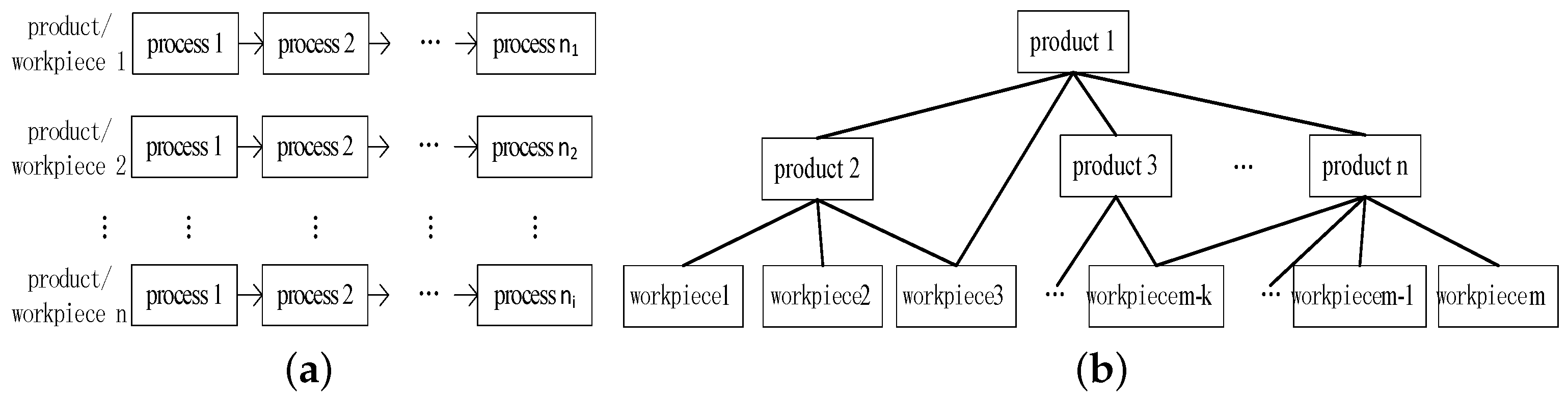
• For a single product, its BOM can be expressed as X = (P, A), in which P is the set of product nodes, A is the relationship matrix of the product nodes, and $a_{ij}$ = 1 indicates that $P_i$ is the child node of $P_j$.

  $$A=\left\{a_{ij}\right\},i,j=1,\dots ,n$$

  (1)

  $$\begin{array}{c}{a}_{ij}=\left\{\begin{array}{c}1,P_i\in P_j^c\\ 0\end{array}\right.\hfill \end{array}$$

  (2)
• The process route is the production process stage of products in different workshops—that is, the process flow between workshops; the process sequence is the internal process of products in each workshop. In the actual production environment, some processes of the product allow the selection of equipment in different workshops, so the problem of equipment balance caused by equipment selection in multi-workshop environment will arise. However, in this paper, we do not elaborate on the balance of multi-workshop equipment. The multi-workshop expression proposed in this paper is to facilitate the elaboration of the production process of the complex products. For the process route and process sequence of a product, it can be expressed as $X^{\prime }$ = (G, W, Q, B, M), in which G is the set of product process routes, W is the set of workshops, Q is the set of product process nodes, B is the relation matrix of process nodes, and M is the set of equipment; $g_{is}$ = 1 means that the product $P_i$ is processed by workshop s, $b_{iskh}$ = 1 means that the process h of $P_i$ in workshop s is the next operation of process k, $b_{iskm}$ = 1 means that the process k of $P_i$ in workshop s is processed by equipment m. For the process route and operation series of a product, it can be expressed as $X^{\prime }$ = (Q, B), in which Q is the process node set of a certain product, B is the relationship matrix of process nodes, $b_{kh}$ = 1 indicates that process h of $P_i$ is the succeeding node of process k.

  $$G=\left\{g_{is}\right\},i=1,\dots ,n;s=1,\dots ,w$$

  (3)

  $$g_{is}=\left\{\begin{array}{c}1,s\in G_i\\ 0\end{array}\right.$$

  (4)

  $$B=\left\{b_{iskh}\right\},k,h=1,\dots ,l;Q_{isk},Q_{ish}\in Q_{is}$$

  (5)

  $$l=L\left(i,s\right)$$

  (6)

  $$b_{iskh}=\left\{\begin{array}{c}1,h=k+1\\ 0\end{array}\right.$$

  (7)

  $$b_{iskm}=\left\{\begin{array}{c}1,m\in M_s\\ 0\end{array}\right.$$

  (8)
• With the organization of product BOM and its process, a process network diagram of the workshop level can be formed; then, further decomposition can be carried out according to the sequence of products in each workshop to form a process-level process network diagram, which can be expressed as $X^{″}$ = (W, N, C, M), in which W is the set of workshops, N is the set of process nodes in the new network diagram, C is the relationship matrix between nodes, M is the set of equipment, $c_{uv}$ = 1 means that process v is the succeeding node of process u, r is the number of nodes, $c_{sum}$ = 1 represents process u of node, and c is processed by equipment m in workshop s.

  $$C=\left\{c_{uv}\right\}u,v=1,\dots ,r$$

  (9)

  $$r=\sum _{i=1}^n\sum _{s=1}^{w}L\left(i,s\right)$$

  (10)

  $$c_{uv}=\left\{\begin{array}{c}1,(Q_{iu},Q_{iv}\in Q_i,v=u+1)\cup (u={\displaystyle \sum _{t=1}^i}{\displaystyle \sum _{s=1}^w}L\left(t,s\right)-1,v={\displaystyle \sum _{t=1}^{j-1}}{\displaystyle \sum _{s=1}^w}L\left(t,s\right)+1,P_i\in P_j^c)\\ 0\end{array}\right.$$

  (11)

  $$c_{sum}=\left\{\begin{array}{c}1,m\in M_s\\ 0\end{array}\right.$$

  (12)
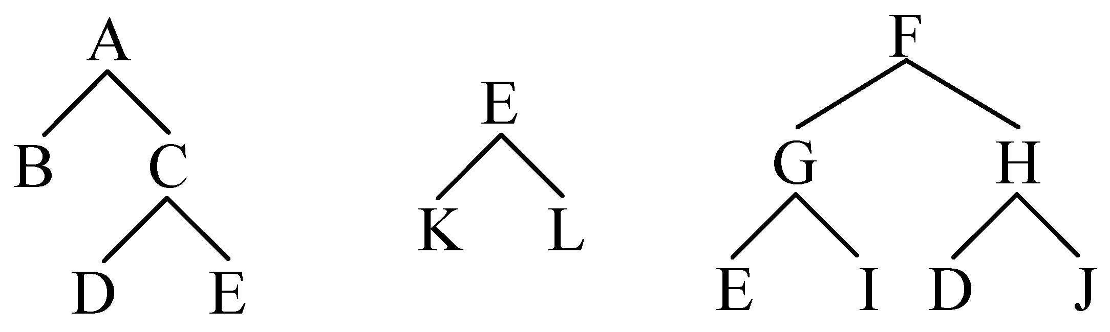
• For multiple products, we can convert the BOM structure according to step 1 for each product. If there are relevant nodes, a merge procedure can be performed, and then the conversion can be performed according to step 2 and step 3. Finally, a complete process network diagram can be created.

For product A~L shown in Figure 3, its process routes are shown in

Table 1. Product process routes.

Product	Process Route	Workshop/ Process Number	Processing Time	Workshop/ Process Number	Processing Time	Workshop/ Process Number	Processing Time
A	W3|W2|W4	W3/2	20—30	W2/2	40—20	W4/3	25—15—30
B	W3|W2	W3/1	50	W2/3	45—25—30
C	W3|W2	W3/2	20—25	W2/2	25—40
D	W4	W4/4	30—20—10—35
E	W3|W4	W3/3	15—15—30	W4/2	30—20
F	W2|W4	W2/2	20—30	W4/3	25—25—35
G	W2|W1	W2/2	25—45	W1/3	20—15—20
H	W4|W2|W3	4/2	15—30	W2/1	30	W3/3	40—20—15
I	W2|W1	W2/1	40	W1/4	10—30—20—20
J	W4|W3	W4/3	30—20—30	W3/2	25—25
K	W1|W4	W1/2	40—20	W4/2	30—10
L	W3|W2	W3/3	20—40—20	W2/4	20—10—30—20

. Product A is composed of B and C, C is composed of D and E, product F is composed of G and H, G and H are composed of E, I and D, J, respectively, and E is composed of K and L. Products A and F both contain part D and assembly E. The process relationship of these products is shown in Table 1. These products are processed or assembled by the equipment in W1~W4 workshops. According to the above steps, it can be converted into a workshop-level process network diagram as shown in Figure 4 and Figure 5, which illustrate the process-level process network diagram after product A’s conversion.

4. Mathematical Model of Scheduling for Multi-Workshop Production

For the scheduling problem of complex products in multi-workshop production, the products and their process constraints can be expressed in the form of a process network diagram, and the scheduling model can be expressed in a set of $\left\{P,Q,F,M,T,TQ\right\}$, and the relevant parameters are shown in

Table 2. Notations.

Symbol	Description
P	Set of all products
$P_i$	Product i, i = 1, …, n
$P_i^p$	Parent node of $P_i$
$P_i^c$	Set of all $P_i$ components
Q	Product process set
$Q_i$	Process set for product $P_i$
$Q_{ik}$	The k-th process of product $P_i$, k = 1, …, l
$LQ$	Number of processes in the product, l = $L{Q}_i$
F	Workshop set
$F_w$	The w-th workshop
M	Set of device resources
$M_{wr}$	The r-th device of workshop w, r = 1, …, m
$M{Q}_{ik}$	Processing device, if process $Q_{ik}$ is processed on device r in workshop w, then $M{Q}_{ik}$ = $M_{wr}$
T	Set of product processing time
$T_i^s$	Start time of product $P_i$
$T_i^e$	Completion time of product $P_i$
$T_i^f$	Required completion time product $P_i$
$TQ$	Set of processing time
$T{Q}_{ik}$	The processing time of the k-th process of product $P_i$—that is, the processing time on the device k in workshop w
$T{Q}_{ik}^s$	Start time of the k-th process of product $P_i$
$T{Q}_{ik}^e$	End time of the k-th process of product $P_i$
$T{Q}_{il}^e$	End time of product $P_i$

. The goal of complex product scheduling is to reasonably arrange the process of products on the premise of ensuring the delivery time, so as to minimize the overall production cycle time. The constraints of the above scheduling problem are as follows:

• Each product can be processed by multiple devices in multiple workshops;
• The workshop where each process is located and the device used by each process are determined;
• At a certain processing time, one device can only be occupied by one process;
• At a certain processing time, a product can only be processed by one device and cannot be interrupted once the process starts;
• The product is processed in the order of its process route, and one process cannot be started until its preceding process is completed;
• The product must follow its BOM structure; that is, the product can start only after all its components have been completed;
• The product should be completed before its delivery date.

For the scheduling problem of n products in a multi-workshop environment, according to the structure of the process network diagram and the above constraints, we can see that each process of the products needs to be processed according to the process network diagram and the constraints on the workshop, device, and process. The ultimate goal is to obtain the optimal processing cycle—that is, to minimize the maximum completion time of each product. The mathematical model of this problem can be expressed as Equation (13):

$$T=min(max(T{Q}_{il}^e))$$

(13)

The constraints can be expressed as:

$$T{Q}_{ik}^e+T{Q}_{ik}\le T{Q}_{i,k+1}^s$$

(14)

$$T{Q}_{ik}^s+T{Q}_{ik}\le T{Q}_{jh}^s,M{Q}_{ik}=M{Q}_{jh}$$

(15)

$$T{Q}_{ik}^e=T{Q}_{ik}^s+T{Q}_{ik}$$

(16)

$$T{Q}_{i1}^s\ge max(T{Q}_{jl}^e),\forall P_j\in P_i^c$$

(17)

$$T{Q}_{\mathrm{i}l}^e\le T_{\mathrm{i}}^f$$

(18)

Equation (14) represents the process route constraint of the product; Equation (15) provides the exclusive constraint of the device; Equation (16) represents the consistency constraint of a single processing; Equation (17) gives the BOM structure constraint of the product; Equation (18) represents the processing cycle constraint of the product.

5. Implementation of Scheduling Algorithm for Multi-Workshop Production

The complex constraints between products and processes need to be considered in the optimization of complex product scheduling, which requires the parallel ability of the algorithm. When the product structure is deep and there are many kinds of products, the process network is more complex, and the parallelism requirement for the solution algorithm is higher. Particle swarm optimization (PSO) is a kind of optimization method based on iteration, which makes individuals accumulate experience continuously through group cooperation, so as to realize the search for the optimal value. Compared with GA and ACO algorithms, the PSO algorithm does not depend on specific problems and has a fast convergence speed. The ACO algorithm has a slow convergence speed, and the search process can easily stagnate due to the consistency of individual solutions. The scheduling of complex products needs to deal with a huge process network diagram, and the algorithm needs to have high search efficiency, so it is not considered to use the ACO algorithm. The GA algorithm, like the PSO algorithm, belongs to the family of bionic algorithms and has parallel search characteristics. PSO particles can preserve the historical experience characteristics and have a certain memory ability, while the experience of the GA algorithm will be destroyed with a change in population. In addition, due to the complex constraints of the process network model, it is difficult to use GA to construct the appropriate coding and operator, which will also affect the efficiency of the algorithm. The PSO algorithm does not have this problem. Therefore, after comprehensive consideration, we select the PSO algorithm to solve the complex product scheduling problem. Since complex product scheduling is a complex optimization problem with multiple constraints and extrema, the standard particle swarm algorithm is prone to premature and low solution accuracy. In this paper, an improved particle swarm algorithm is proposed, which changes the direction and speed of the particles through recombination, improves the diversity of the population, and prevents the algorithm from prematurely converging. In addition, by setting the dynamic inertia weight, the global search ability of the algorithm is improved. In the standard particle swarm algorithm, the initial particle swarm is generated randomly, and the optimal solution is obtained through continuous iteration. After each iteration, the individual extremum and global extremum are updated by the fitness value, and the velocity and position are updated according to the equation. As shown in Equations (19) and (20):

$$V_{i,j}^{t+1}=\omega V_{i,j}^t+c_1{r}_1(P_{i,j}-X_{i,j}^t)+c_2{r}_2(g_j-X_{i,j}^t)$$

(19)

$$X_{i,j}^{t+1}=V_{i,j}^{t+1}+X_{i,j}^t$$

(20)

$X_{i,j}^t$ and $V_{i,j}^t$ represent the position and velocity of the i-th (i = 1, 2, 3, …, n) particle in the j dimension (j = 1, 2, 3, …, m) after the t-th (t = 1, 2, 3, …, T) iteration; P represents the optimal value of the i-th particle in the j-th dimension; $\omega$ represents the inertia weight, which decreases linearly with the increase in iteration time, and the convergence effect is better when $\omega$ is between 0.8 and 1.2; g is the global optimal value; c1 and c2 represent learning factors; r1 and r2 represent random numbers that obey random distribution in the interval (0, 1).

5.1. Encoding and Decoding Mechanism

Coding is the key to the successful implementation of particle swarm optimization. In this paper, the coding method based on the process is adopted, and an operation sequence vector is used to represent a scheduling scheme. The operation of each workpiece in the vector is represented by the corresponding workpiece serial number. Scan the particles from left to right, and the number of the workpiece that appears for the k-th time indicates the k-th process of the workpiece. For example, a sequence vector (particle) is (1-3-2-3-1-1-3-2-2), and the processing order of its corresponding operation sequence is Q11-Q31-Q21-Q32-Q12-Q13-Q33-Q22-Q23. Each sequence node acts as a particle, and the whole process sequence forms a particle swarm.

5.2. Generation of Initial Particle Swarm

According to the process network diagram and mathematical model of complex product scheduling proposed in the previous section, the initial population can be obtained according to the following steps.

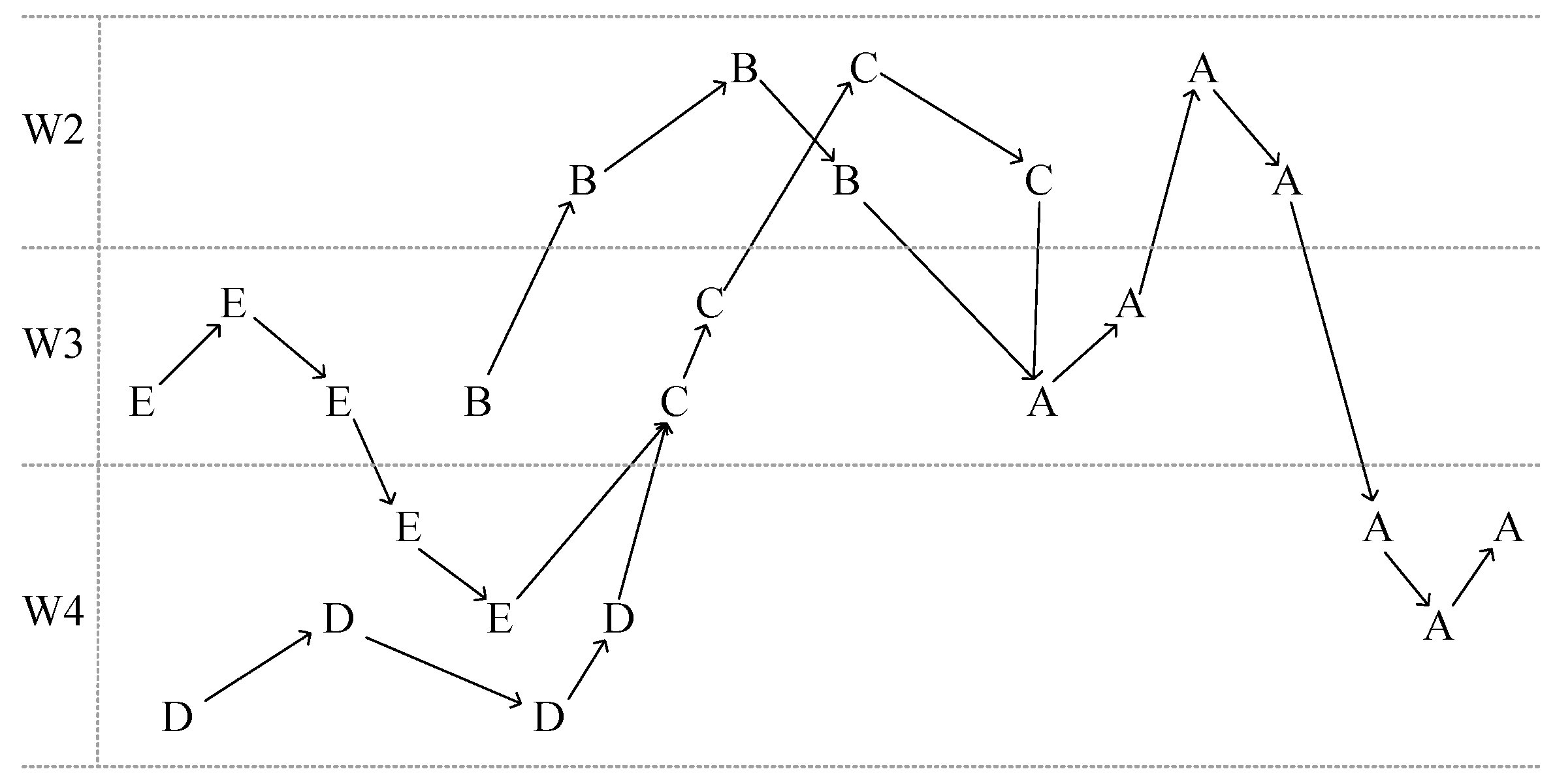
• The process network graph G of complex product scheduling is established, and a node is selected as the first node of the operation sequence from each initial node without forward node in G.
• Remove the node in (1) from the network graph G to form a new process network graph $G^{\prime }$; $G^{\prime }$ is a subgraph of G. The next node is randomly selected in the graph $G^{\prime }$, and only the node without the forward node in $G^{\prime }$ can be selected.
• Repeat the process (2). The construction process of $G^{\prime }$ is shown in Figure 5. In this way, the validity of the sequence can be ensured. As shown in the figure, until all nodes have joined the operation sequence, the obtained operation sequence can be used as the initial particle swarm.

5.3. Improvement of Population Evolutionary Diversity

In the standard particle swarm algorithm, the operation of particles is affected by individual experience and group experience. If a particle is in the current optimal position, other particles will quickly approach it. However, if the optimal position is a local extremum, then the particle swarm can easily fall into the local optimum and cannot re-search in the solution space, which leads to the premature phenomenon of the algorithm. In order to overcome premature convergence and improve population diversity, if the global extremum remains unchanged after the iterative operation, the historical optimal positions of m (m < N/10) particles are randomly selected and recombined with the current generation particles, as shown in Equation (21).

$$S_{new}(x_i)=\sum _{k=1}^m\left(r_c{S}_p(x_k)+(1-r_c)\left|S_c(x_i)-S_p(x_k)\right|\right)/\phantom{\sum _{k=1}^m\left(r_c{S}_p(x_k)+(1-r_c)\left|S_c(x_i)-S_p(x_k)\right|\right)m}m$$

(21)

Among them, $S_{new}$ represents the newly generated particle; $S_p$ represents the selected historical optimal position; $S_c$ represents the current particle; $r_c$ represents a random number between (0, 1). The new particles have different running directions and speeds, so they can explore new search spaces, jump out of the local optimum, and avoid premature convergence. In addition, the use of historical best involves using the best location searched by the individual as a reference and searching around it, hoping to identify a better location, which is conducive to continuously improving the quality of the solution and ensuring the optimization accuracy on the basis of increasing the diversity of particles.

5.4. Dynamic Inertia Weight

The inertia weight $\omega$ reflects the impact of the particle’s previous velocity on this generation. In the standard particle swarm algorithm, $\omega$ is linearly decreasing. Usually, the value of $\omega$ is larger in the early stage of algorithm optimization, which is beneficial to the global optimization. At the end of the iteration, the value of $\omega$ is smaller, which is beneficial to local optimization. In this article, the following improvements are made to $\omega$.

$$\omega (t)=r_{\omega }({\omega }_{max}-{\omega }_{min})exp(-\frac{t}{T}{({\omega }_{max}-{\omega }_{min})}^2)$$

(22)

In Equation (22), $r_{\omega }$ is a weight coefficient with a value less than 1. Different from the linear decreasing model, this equation represents a dynamic inertia weight. The decreasing speed is more suitable for the particle search process and better balances the global search ability and local search ability of the algorithm.

5.5. Algorithm Implementation Steps

The main steps of the improved PSO algorithm are as follows.

• Step 1: Parameter setting, including population size, maximum number of iterations n, learning factor, upper and lower limits of particle position and speed, dimension of the algorithm (this paper takes the total number of operation nodes as the dimension).
• Step 2: Initialize the population by using the coding method based on operation and the method shown in Figure 6.
• Step 3: Update the particles, update the speed and position according to Equations (19) and (20), and calculate the individual extreme and global extreme.
• Step 4: If the global extremum remains unchanged, a new generation of particles will be generated according to Equation (21). Otherwise, step 4 will be adjusted to step 5.
• Step 5: Update the inertia weight according to Equation (22).
• Step 6: Depends on whether the termination condition is satisfied. If not, return to step 3. Otherwise, the optimal solution is output and the algorithm ends.

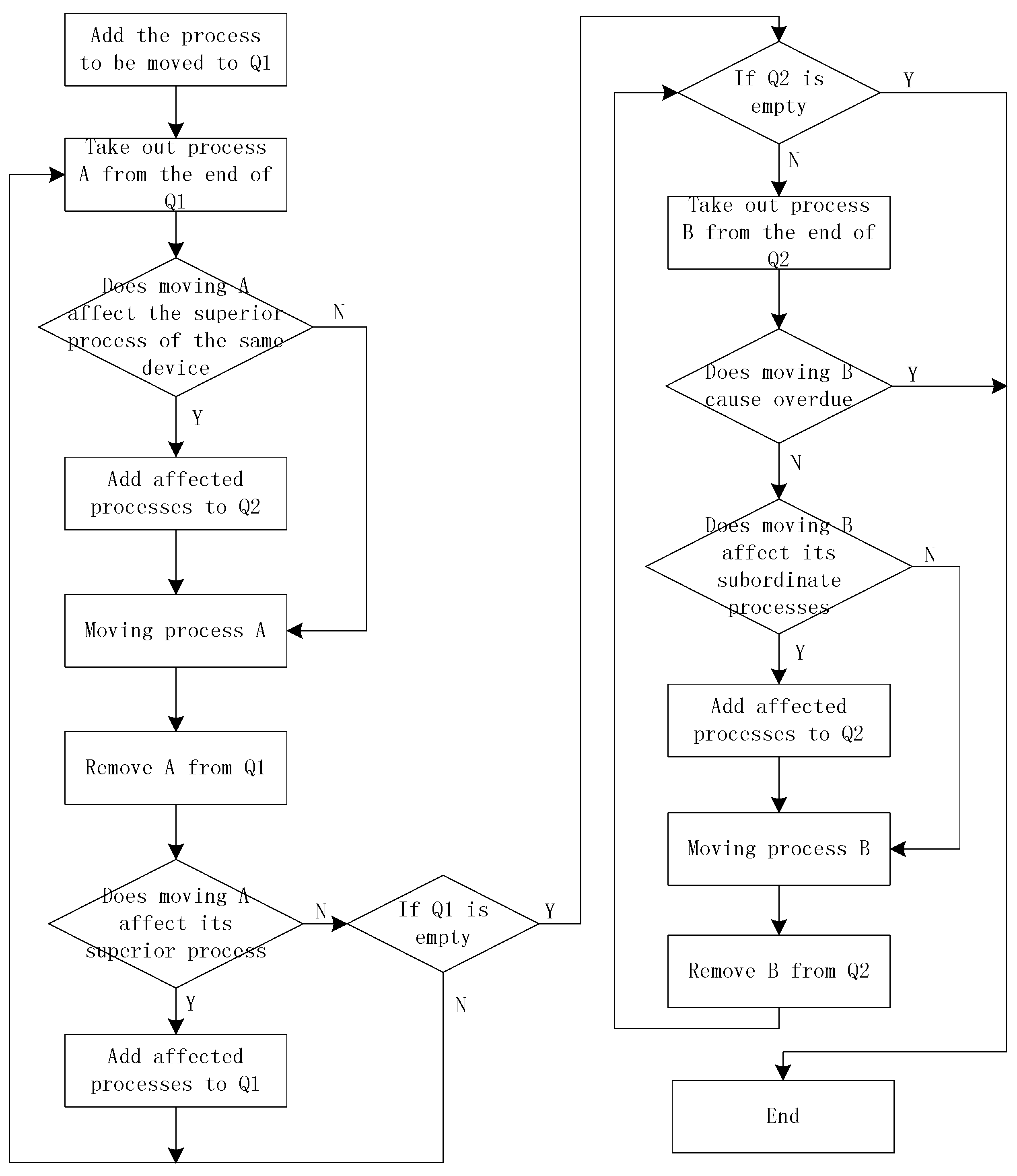
6. Treatment of Time Constraints

When there is a time limit, a large number of invalid paths will be generated in the process of algorithm evolution. To solve this problem, we can assign priority weight to activities and search nodes with high priority first. The assignment of priority weight values needs to consider the following aspects:

• Product delivery cycle: the weight coefficient can be set according to the product delivery cycle, and it is valid for all nodes of the product;
• Level/complexity of the product: the farther the subordinate node is from the top node of the product, the higher the weight is required;
• Number of peer nodes: the more peer nodes one node has, the higher weight the node needs to be assigned;
• Process route and processing time: the longer the process flow and processing time are, the higher the weight required;
• The flexibility of the search needs to be ensured, and the search process can be limited according to the range of weights.

The above method of priority assignment can ensure that the searched path is an effective path. The space for path search depends on the restriction of weight usage. If the restriction is strict, it is easy for the algorithm to fall into a local optimum, and if the restriction is loose, it will cause an invalid path. The priority weight value of the activity allocation can be determined by AHP (analytic hierarchy process). AHP is a practical multi-objective decision-making method. Using this method to analyze problems generally includes four steps: the goal of decision-making, the factors considered, and the decision-making object are layered according to their mutual relationship, and the hierarchical structure diagram is drawn; the judgment matrix is constructed to determine the weight of each factor at each level; the single-level ranking is carried out—that is, for a factor at the upper level, the importance of each factor is ranked, and the consistency test is carried out; the hierarchical total ranking is to calculate the weight of the relative importance of all factors at a certain level to the total goal, which is carried out from the highest level to the lowest level in turn. However, the method of priority weight assignment has the problem of the search space being too small. In this regard, this study proposed a new path search strategy, the path search rescheduling strategy, which does not limit the range of the path search. This strategy is suitable for some products with time constraints and can ensure that effective search paths are obtained.

The path search rescheduling method adjusts the products that do not meet the schedule constraints and adjusts other products that do not meet the schedule constraints caused by this adjustment. Through this traversal adjustment, all products finally meet the schedule requirements. For the search path 4-5-3-2-1-7-8-6 shown in Figure 7, if the delivery cycle of product 6 is at 7, Figure 7a indicates that the scheduling cannot meet the requirements, and the cycle of product 1 is lost; then, product 6 can be moved before product 1, and its subordinate product 7 needs to be moved to the front of product 2 to form a new search path, as shown in Figure 7b. Then, both products 1 and 6 meet the scheduling requirements. The implementation of the path search rescheduling strategy is shown in Figure 8.

In the figure above, Q1 and Q2 represent the sets of processes to be moved and affected, respectively. The implementation process of path search rescheduling is divided into two processes, respectively, for Q1 and Q2. In the flow on the left side of the diagram, first add the process that needs to be moved to Q1, and check whether moving process A at the end of Q1 will affect other processes of the same device. If no, move process A directly. If yes, add the affected process to Q2. Delete process A from Q1, then judge whether moving process A will affect its superior processes. If yes, add the affected process to Q1. Otherwise, check whether Q1 is empty. If Q1 is not empty, return to the flow on the left to continue the above operation. If Q1 is empty, enter the flow on the right side of the diagram. If Q2 is empty, end the flow. If Q2 is not empty, take out the process B from the end of Q2, and check whether move B is overdue; end the process if yes. Otherwise, move process B and check whether move B will affect its subsequent processes. If not, move B. Otherwise, move B after adding the affected processes. Delete B from Q2, and return to the flow on the right side to continue the above operation.

7. A Case Study

In order to verify the feasibility and performance of the model and algorithm proposed in this paper, the product in Figure 3 is taken as an example. In this example, this case study consists of 12 products/workpieces, 61 processes, and 4 workshops. The parameters of PSO are set as follows: T = 100, N = 15, c1 = 2, c2 = 2. The fluctuation range of $\omega$ is (0.8, 1.2), the particle velocity range is in (−0.8, 0.8), and the particle position is limited in the range of the workpiece serial number. The calculation results of the model are shown in the figure below.

Figure 9 shows the fitness evolution curve of the optimized scheduling of each round of iteration, Figure 10a illustrates the initial scheduling sequence, and Figure 10b shows the optimized scheduling sequence after 100 iterations.

In order to confirm the effectiveness of the algorithm, the algorithm in this paper is compared with the ant colony algorithm and genetic algorithm. After analyzing the convergence and stability of different algorithms, the experimental data obtained by comparison are shown in Figure 11. The parameters of the genetic algorithm are as follows: the number of populations is 10, the crossover probability is 0.4, the mutation probability is 0.2, and the normalized elimination acceleration index is 1.5. The parameters of ant colony algorithm are set as follows: number of ant colonies is 15, heuristic factor is 3, expected heuristic factor is 3, information intensity is 20, pheromone evaporation factor is 0.5, and the iterations of the three algorithms are 100.

Figure 11a shows the comparison of the scheduling optimization results of the three algorithms for 30 products and 107 processes, and Figure 11b shows the comparison of the scheduling optimization results for 70 products and 225 processes. It can be seen from the results in the figure that, in the two examples, the improved particle swarm optimization algorithm used in this paper has achieved good results. In order to evaluate the performance of different algorithms, this paper further tests six cases with different numbers of products, processes, workshops, and equipment and records the search results of each algorithm, as shown in

Table 3. Comparison of resource balance optimization of different project network plans.

Products	Processes	Workshops	Devices	Pre Value	GA		PSO		ACO
					Optimal Value	Average Value	Optimal Value	Average Value	Optimal Value	Average Value
10	35	2	6	640	433	440	456	456	483	521
20	71	2	10	1001	572	601	590	590	714	759
30	107	3	12	1100	796	820	867	873	840	866
50	183	4	16	1626	962	994	998	998	976	1006
70	225	5	22	1128	572	591	639	645	587	602
100	291	6	30	1318	775	843	889	896	823	893

.

Through the analysis of Table 3, we can find that the algorithm and GA algorithm can obtain better scheduling results for case 1 and 2 with fewer products; for case 3 and 4, the algorithm in this paper is similar to the other two algorithms, but it is still better than the other two algorithms; in case 5 and 6, with the increase in the product number, the optimal value of this algorithm is still better than the other algorithms. This shows that the algorithm can not only obtain a better solution but also has strong stability, which is not random or accidental.

Figure 12a shows the scheduling result analysis when the product quantity and process route remain unchanged and the product complexity increases. The three curves respectively correspond to the worst value, the best value, and the average value of the scheduling result. It can be seen that the product complexity has a positive relationship with the scheduling result. Figure 12b shows the scheduling result analysis when the product quantity and product complexity remain the same while the process route increases. It can be seen that the process route is in a reverse relationship with the scheduling result at the beginning, and then tends to be synchronous. Figure 12c shows the scheduling result analysis when the complexity of process route and product remains unchanged while the number of products increases. It can be seen that there is a positive relationship between product quantity and scheduling results.

Figure 13 is a comparison of the scheduling results for 100 products and 291 processes. From the computation results of the above case study, it can be seen that, under the premise of satisfying the constraints of product structure and process route, the optimized scheduling sequence has a significantly shorter completion cycle than the initial scheduling sequence. At the same time, after adding products, processes, workshops, and device, although the data scale becomes larger, compared with the average scheduling result, the optimized scheduling result is not affected and remains in a stable improvement interval. Therefore, the algorithm designed in this study has strong robustness for the scheduling of complex products in multi-workshop production.

8. Conclusions

This paper presented a study of the scheduling problem in multi-workshop production. Based on the study of the BOM composition and process route constraints of complex products, and with the goal of minimizing the production cycle of all products, a method for constructing a complex product process network diagram was proposed. The network diagram construction methods of a single product, multiple products, and related products were given. Then, the mathematical model of scheduling for multi-workshop production was created. An improved particle swarm algorithm was developed to solve the problem. The algorithm was improved from two aspects of particle recombination and inertia weight, overcoming the problem of premature convergence and improving the diversity of the population. In addition, to solve the problem of an invalid path in the process of searching with time constraints, a path search rescheduling strategy was proposed to ensure that a valid path could be obtained. In the case study, the model and algorithm were verified by several different examples and compared with GA and the ACO algorithm. The results show that the proposed model and algorithm are better, and the model and algorithm proposed in this study can effectively solve the scheduling problem involving complex products in multi-workshop production. In terms of resource capability, this research adopted a simplified resource model. The selection of similar device resources in different workshops is worth further research. The above methods can be improved by combining resource sharing and conflict mediation mechanisms in scheduling optimization.

References

1. Zhao, B.; Gao, J.; Chen, K.; Guo, K. Two-generation Pareto ant colony algorithm for multi-objective job shop scheduling problem with alternative process plans and unrelated parallel machines. J. Intell. Manuf. 2018, 29, 93–108. [Google Scholar] [CrossRef]
2. Luo, Y. Nested optimization method combining complex method and ant colony optimization to solve JSSP with complex associated processes. J. Intell. Manuf. 2017, 28, 1801–1815. [Google Scholar] [CrossRef]
3. Li, C.; Shen, H.; Li, L.; Yi, Q. A Batch Splitting Flexible Job Shop Scheduling Model for Energy Saving under Alternative Process Plans. J. Mech. Eng. 2017, 53, 12. [Google Scholar] [CrossRef]
4. Huang, X.; Zhang, X.; Ai, Y. ACO integrated approach for solving flexible job-shop scheduling with multiple process plans. Comput. Integr. Manuf. Syst. 2018, 24, 558–569. [Google Scholar]
5. Naderi, B.; Azab, A. An improved model and novel simulated annealing for distributed job shop problems. Int. J. Adv. Manuf. Technol. 2015, 81, 693–703. [Google Scholar] [CrossRef]
6. Ackermann, S.; Fumero, Y.; Montagna, J.M.M. Optimization Framework for the Simultaneous Batching and Scheduling of Multisite Production Environments. Ind. Eng. Chem. Res. 2018, 57, 16395–16406. [Google Scholar] [CrossRef]
7. Asl, A.J.; Solimanpur, M.; Shankar, R. Multi-objective multi-model assembly line balancing problem: A quantitative study in engine manufacturing industry. OPSEARCH 2019, 56, 603–627. [Google Scholar]
8. Azami, A.; Demirli, K.; Bhuiyan, N. Scheduling in aerospace composite manufacturing systems: A two-stage hybrid flow shop problem. Int. J. Adv. Manuf. Technol. 2018, 95, 3259–3274. [Google Scholar] [CrossRef]
9. Li, W.; He, L.; Cao, Y. Many-Objective Evolutionary Algorithm With Reference Point-Based Fuzzy Correlation Entropy for Energy-Efficient Job Shop Scheduling With Limited Workers. IEEE Trans. Cybern. 2021, 554, 236–255. [Google Scholar]
10. Gao, K.; Cao, Z.; Zhang, L.; Chen, Z.; Han, Y.; Pan, Q. A Review on Swarm Intelligence and Evolutionary Algorithms for Solving Flexible Job Shop Scheduling Problems. IEEE/CAA J. Autom. Sin. 2019, 6, 904–916. [Google Scholar] [CrossRef]
11. Knopp, S.; Dauzère-Pérès, S.; Yugma, C. A Batch-Oblivious Approach for Complex Job-Shop Scheduling Problems. Eur. J. Oper. Res. 2017, 263, 50–61. [Google Scholar] [CrossRef]
12. Dai, Y.J.; Zhang, Z.Y.; Wang, W.Z. Block two-stage and multi-workshop scheduling with transportation consideration. Comput. Eng. Appl. 2016, 52, 222–228. [Google Scholar]
13. Yeganeh, F.T.; Zegordi, S.H. A multi-objective optimization approach to project scheduling with resiliency criteria under uncertain activity duration. Ann. Oper. Res. 2020, 285, 161–196. [Google Scholar] [CrossRef]
14. Delice, Y. A genetic algorithm approach for balancing two-sided assembly lines with setups. Assem. Autom. 2019, 39, 827–839. [Google Scholar] [CrossRef]
15. Jiang, Z.Q.; Le, Z.; Mechanical, S.O. Multi-objective flexible job-shop scheduling based on low-carbon strategy. Comput. Integr. Manuf. Syst. 2015, 21, 1023–1031. [Google Scholar]
16. Elmi, A.; Topaloglu, S. Multi-degree cyclic flow shop robotic cell scheduling problem: Ant colony optimization. Comput. Oper. Res. 2016, 30, 805–821. [Google Scholar] [CrossRef]
17. Ziaee, M. A heuristic algorithm for the distributed and flexible job-shop scheduling problem. J. Supercomput. 2014, 67, 69–83. [Google Scholar] [CrossRef]
18. Le, H.T.; Geser, P.; Middendorf, M. An Iterated Local Search Algorithm for the Two-Machine Flow Shop Problem with Buffers and Constant Processing Times on One Machine. In Proceedings of the European Conference on Evolutionary Computation in Combinatorial Optimization (Part of EvoStar), Leipzig, Germany, 24–26 April 2019; pp. 50–65. [Google Scholar]
19. Zhang, G. Hybrid variable neighborhood search for multi objective flexible job shop scheduling problem. In Proceedings of the 2012 IEEE 16th International Conference on Computer Supported Cooperative Work in Design (CSCWD), Wuhan, China, 23–25 May 2012; pp. 725–729. [Google Scholar]
20. Nagano, M.S.; Komesu, A.S.; Miyata, H.H. An evolutionary clustering search for the total tardiness blocking flow shop problem. J. Intell. Manuf. 2019, 30, 1843–1857. [Google Scholar] [CrossRef]
21. Cao, Y.; Zhang, H.; Li, W.; Zhou, M.; Zhang, Y.; Chaovalitwongse, W.A. Comprehensive Learning Particle Swarm Optimization Algorithm With Local Search for Multimodal Functions. IEEE Trans. Evol. Comput. 2019, 23, 718–731. [Google Scholar] [CrossRef]
22. Lv, Z.; Wang, L.; Han, Z.; Zhao, J.; Wang, W. Surrogate-Assisted Particle Swarm Optimization Algorithm With Pareto Active Learning for Expensive Multi-Objective Optimization. IEEE/CAA J. Autom. Sin. 2019, 6, 838–849. [Google Scholar] [CrossRef]
23. Liu, T.K.; Chen, Y.P.; Chou, J.H. Solving Distributed and Flexible Job-Shop Scheduling Problems for a Real-World Fastener Manufacturer. IEEE Access 2014, 2, 1598–1606. [Google Scholar]
24. Liang, J.; Wang, P.; Guo, L.; Qu, B.; Yue, C.; Yu, K.; Wang, Y. Multi-objective flow shop scheduling with limited buffers using hybrid self-adaptive differential evolution. Memetic Comput. 2019, 11, 407–422. [Google Scholar] [CrossRef]
25. Wang, S.; Wang, L.; Liu, M.; Xu, Y. An estimation of distribution algorithm for the multi-objective flexible job-shop scheduling problem. In Proceedings of the 2013 IEEE Symposium on Computational Intelligence in Scheduling (CISched), Singapore, 16–19 April 2013; pp. 1–8. [Google Scholar]
26. Gen, M.; Zhang, W.; Lin, L.; Yun, Y. Recent advance in hybrid evolutionary algorithms for multiobjective manufacturing scheduling. Comput. Ind. Eng. 2017, 112, 616–633. [Google Scholar] [CrossRef]
27. Kucukkoc, I.; Zhang, D.Z. Integrating ant colony and genetic algorithms in the balancing and scheduling of complex assembly lines. Int. J. Adv. Manuf. Technol. 2016, 82, 265–285. [Google Scholar] [CrossRef] [Green Version]
28. Wong, T.N.; Zhang, S.; Wang, G.; Zhang, L. Integrated process planning and scheduling-multi-agent system with two-stage ant colony optimization algorithm. Int. J. Prod. Res. 2012, 50, 6188–6201. [Google Scholar] [CrossRef]
29. Chen, Z.; Zheng, X.; Zhou, S.; Liu, C.; Chen, H. Quantum-inspired ant colony optimization algorithm for a two-stage permutation flow shop with batch processing machines. Int. J. Prod. Res. 2020, 58, 5945–5963. [Google Scholar] [CrossRef]
30. Duan, J.H.; Meng, T.; Chen, Q.D.; Pan, Q.K. An Effective Artificial Bee Colony for Distributed Lot-Streaming Flow-shop Scheduling Problem. In Proceedings of the Intelligent Computing Methodologies, Wuhan, China, 15–18 August 2018; pp. 795–806. [Google Scholar]
31. Shivasankaran, N.; Kumar, P.S.; Raja, K.V. Hybrid Sorting Immune Simulated Annealing Algorithm For Flexible Job Shop Scheduling. Int. J. Comput. Intell. Syst. 2015, 8, 455–466. [Google Scholar] [CrossRef] [Green Version]
32. Golmakani, H.R.; Birjandi, A.R. A two-phase algorithm for multiple-route job shop scheduling problem subject to makespan. Int. J. Adv. Manuf. Technol. 2013, 67, 203–216. [Google Scholar] [CrossRef]
33. Zhuang, C.B.; Xiong, H.; Liu, J.H.; Tang, C.T. An Improved Discrete Krill Herd Algorithm for Complex Product Assembly Scheduling Problem. Acta Armamentarii 2018, 39, 1590–1600. [Google Scholar]
34. Lei, D.; Wang, T. Solving distributed two-stage hybrid flow shop scheduling using a shuffled frog-leaping algorithm with memeplex grouping. Eng. Optim. 2019, 12, 1–14. [Google Scholar]
Figure 1. Product processing and assembly process. (a) Product/workpiece manufacturing process flow, (b) Product assembly composition relationship.
Applsci 11 05078 g001
Figure 2. Composition of a complex product assembly.
Applsci 11 05078 g002
Figure 3. BOM structure of product A.
Applsci 11 05078 g003
Figure 4. Workshop-level process network diagram conversion for product A.
Applsci 11 05078 g004
Figure 5. Process-level process network diagram conversion for product A.
Applsci 11 05078 g005
Figure 6. Construction of the process network subgraph.
Applsci 11 05078 g006
Figure 7. An example of path search rescheduling strategy. (a) Not meeting the requirements before adjustment, (b) Meet the requirements after adjustment.
Applsci 11 05078 g007
Figure 8. Implementation of the path search rescheduling strategy.
Applsci 11 05078 g008
Figure 9. Iterative fitness evolution curve.
Applsci 11 05078 g009
Figure 10. Comparison of results before and after scheduling optimization. (a) Initial scheduling sequence, (b) Optimal scheduling sequence.
Applsci 11 05078 g010
Figure 11. Comparison of target value curves of three algorithms. (a) Comparison example 1, (b) Comparison example 2.
Applsci 11 05078 g011
Figure 12. Influence of product complexity, process route, and product quantity on scheduling results. (a) Analysis of the impact of product complexity on scheduling results, (b) Analysis of influence of process route on dispatching results, (c) Analysis of the impact of product quantity on scheduling results.
Applsci 11 05078 g012
Figure 13. Comparison of results before and after scheduling optimization (100 products). (a) Initial scheduling sequence, (b) Optimized scheduling sequence.
Applsci 11 05078 g013