Multi-Feature Guided Low-Light Image Enhancement

Abstract

Due to the characteristics of low signal-to-noise ratio and low contrast, low-light images will have problems such as color distortion, low visibility, and accompanying noise, which will cause the accuracy of the target detection problem to drop or even miss the detection target. However, recalibrating the dataset for this type of image will face problems such as increased cost or reduced model robustness. To solve this kind of problem, we propose a low-light image enhancement model based on deep learning. In this paper, the feature extraction is guided by the illumination map and noise map, and then the neural network is trained to predict the local affine model coefficients in the bilateral space. Through these methods, our network can effectively denoise and enhance images. We have conducted extensive experiments on the LOL datasets, and the results show that, compared with traditional image enhancement algorithms, the model is superior to traditional methods in image quality and speed.

1. Introduction

When the object is in a low-light environment, such as backlight, at night, or the image is underexposed during the capture process, the resulting low-light image will affect visual perception and lose information. The loss of image information will cause many adverse effects. For example, in the target detection task at night, it will cause the accuracy of the detection results to be reduced, and even missed and false detections.

Image enhancement based on low-light images is a current research hotspot and difficulty in the field of image processing. This technology is widely used, and most commonly used to enhance photos taken by the camera at night or in other low-light scenes. Chen et al. [1] propose a new image processing pipeline to avoid the noise amplification and error accumulation problems caused by traditional camera processing pipelines. Guo et al. 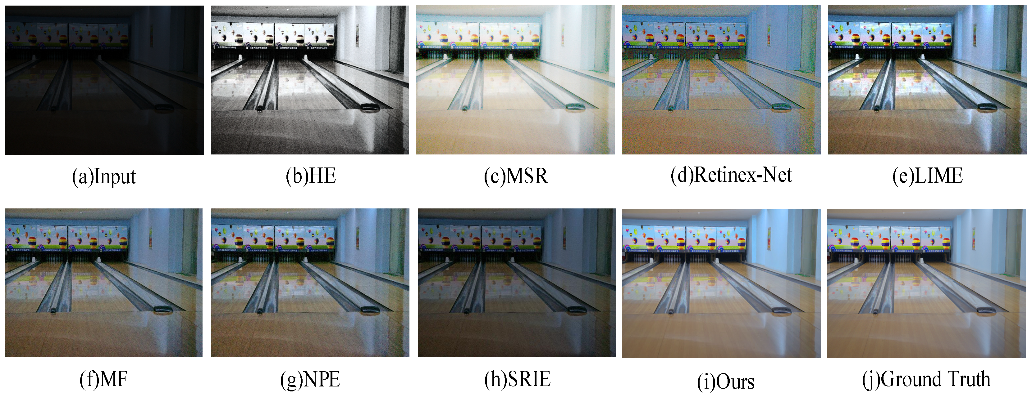[2] combine this method with target detection technology to improve the accuracy of detecting targets at night. However, due to its own characteristics, low-light images are often mixed with a lot of noise, which increases the difficulty of image enhancement. In order to achieve the desired enhancement effect, researchers have proposed many ideas and methods. In the early days, high-quality images were obtained by enhancing image contrast; the representative method is histogram equalization. However, this type of method is incapable of restoring image details and colors. With the development of deep learning in recent years, data-driven neural network methods have also been widely adopted and improved. The neural network-based method can learn more complex color and contrast transformations and has strong expressive power, but there are still many problems. The current mainstream traditional image enhancement methods and the existing problems of neural network enhancement methods are shown in Figure 1:

It can be seen from Figure 1 that traditional models such as histogram equalization (HE) [3] only consider contrast enhancement when enhancing images, while Retinex-Net [4] and NPE [5] methods will cause serious color distortion. Methods such as MF [6], LIME [7], SRIE [8], and MSR [9] are lacking both in image quality and visual expressiveness, which affect the sensory aesthetics and later target detection work.

In this paper, we propose a new deep neural network architecture to enhance low-light images. For noise removal and illumination enhancement, feature maps are extracted through two sub-networks to obtain noise and illumination features. Then, it is guided by the extracted features, and the denoising and enhancement work are performed at the same time, which avoids the limitations caused by the first enhancement and then the denoising, or the first denoising, and then the enhancement. In addition, we also use the method of bilateral grid upsampling to accelerate the image processing process and achieve the purpose of fast image enhancement without reducing the image quality.

2. Related Work

From the emergence of digital image processing technology to the present, image enhancement technology has made considerable progress. In recent years, with the rise of target detection, more and more low-light image enhancement and denoising algorithms have been proposed.

Enhancing the image by changing the contrast is an early classic idea, such as histogram equalization (HE) and an improved version of the contrast-limited adaptive histogram equalization (CLAHE) [10]; the principle is to increase the contrast by expanding the dynamic range of image pixel values and reducing the image gray level. Another method is gamma correction (GC), which changes the contrast by multiplying each pixel. The limitation of these two types of methods lies in the global adjustment of the image, and the resulting image will be distorted.

Retinex theory [11] believes that the object has color constancy, and the image can be expressed as reflection and illumination. Early methods based on this theory include single-scale Retinex (SSR) [12] and multi-scale Retinex (MSR) [9]. The output of this method tends to be unnatural and locally over-enhanced. Fu et al. [8] proposed a weighted change model to estimate the reflection and illumination of the input image. In the same year, they proposed an image enhancement method based on the fusion idea [6], which adjusted the illumination image through multi-scale fusion and weighted average strategy. Cai et al. [13] adjusted the image by combining texture and illumination priors. LIME [4] designed a structure-aware smoothing model to predict the illumination map. Martin et al. [14] proposed a robust Retinex model, which introduced noise feature maps for denoising enhancement. The method based on Retinex theory is to estimate the illumination map by decomposing the image, and then enhancing the illumination map. This kind of method depends on the accuracy of image decomposition, but often the decomposed components are not exactly the same, so the enhanced image obtained is less authentic, and noise will inevitably be added and amplified.

Deep learning methods have shown unprecedented potential in learning image enhancement. Wei et al. [4] combined Retinex and deep learning methods to propose Retinex-net. This network decomposes the image, and under the assumption of smooth illumination map, the reflection component is denoised by the BM3D method, and finally the image is reconstructed. However, this method will cause color distortion and unsatisfactory noise removal effect. Wang et al. [15] introduced an intermediate illumination layer in the network for image enhancement and learned the image adjustment ability through image data carefully designed by experts. Chen et al. [16] proposed an image enhancement method for processing unpaired datasets based on a two-way generative confrontation network. GHARBI et al. [17] performed most of the processing at low resolution and used deep bilateral models for fast image enhancement. Chen et al. [1] proposed a fully convolutional network model that can be trained end-to-end for processing low-light images.

As low-light image enhancement is an ill-posed problem, no ground truth is available in the real situation. Therefore, there are many deep learning methods for low-light image enhancement based on unpaired or self-supervision. Guo et al. [2] set a series of non-reference loss functions to enable the network to perform end-to-end training without any reference images. Jiang et al. [18] proposed an efficient and unsupervised generative adversarial network called EnlightenGAN for the low-light image enhancement problem, which can be trained without low/normal-light image pairs. N. Anantrasirichai and David Bull [19] used an adaptation of the CycleGan structure to color and denoise images. They also proposed a multiscale patch-based framework, capturing both local and contextual features. Lehtinen et al. [20] thought it possible to learn to restore images by only looking at corrupted examples without explicit image priors or likelihood models of the corruption.

Image denoising: image denoising is an indispensable work for image processing. In recent years, many denoising methods and ideas have emerged. According to ideas, denoising algorithms can be divided into conversion algorithms and spatial algorithms. The most classic conversion algorithm is wavelet transform, while non-local means (NL-means) is a classic spatial algorithm. At the same time, there is also the well-known BM3D [21] algorithm that combines the two ideas. This algorithm has a good effect on the current normal image denoising effect, but it has great defects in the speed and low-illumination image denoising. In addition, deep learning methods also have strong expressive power in image denoising. REDNet [22] built an encoding and decoding network to learn image denoising. CBDNet [23] denoised real images by establishing a noise model that is closer to the real world and based on asymmetric learning.

3. Materials and Methods

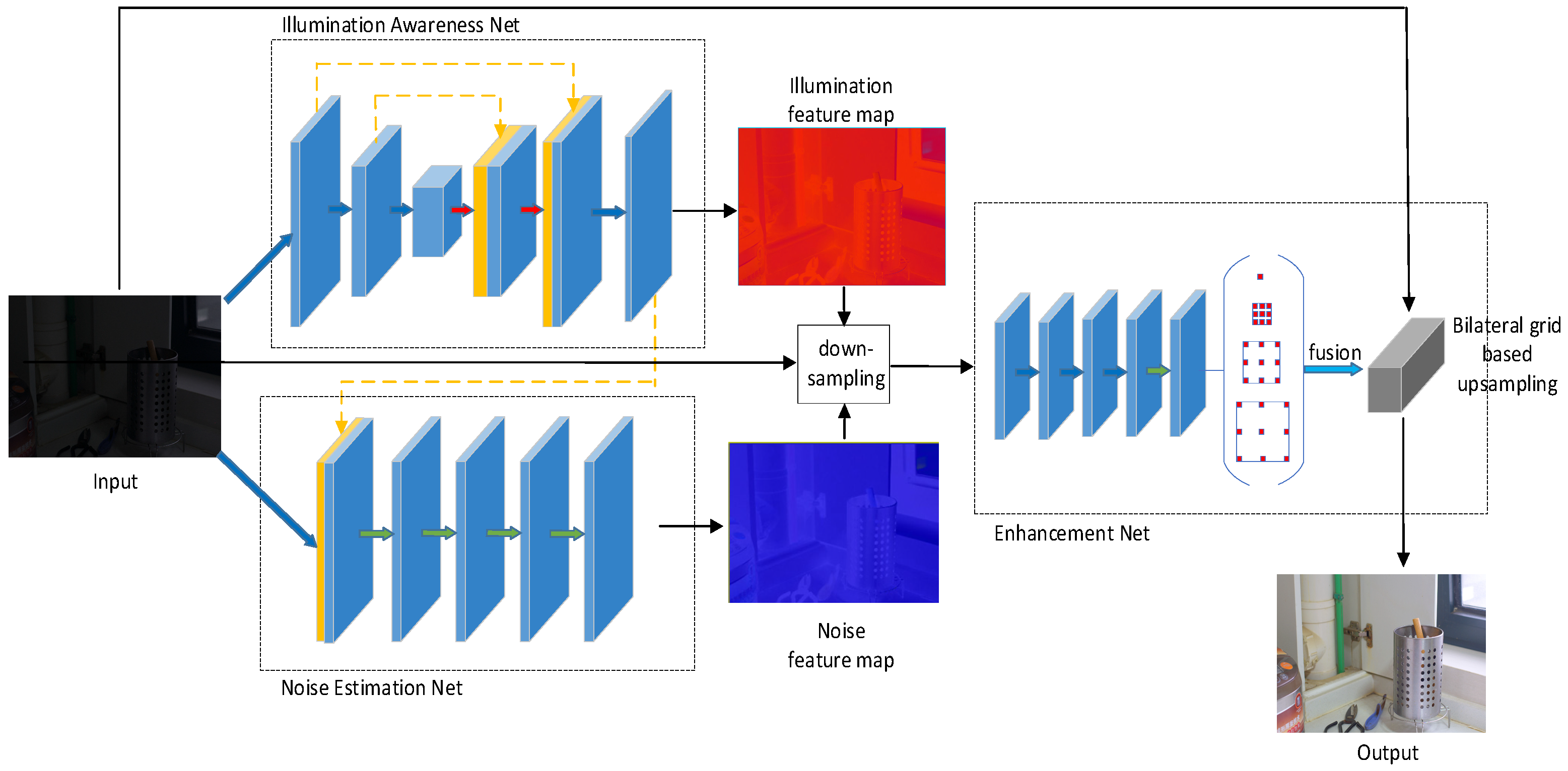
In this paper, we consider the impact of low-light image noise and propose a multi-feature guided model with illumination map and noise map. After training, it can quickly remove noise and enhance image at the same time and can also retain the detailed information of the image. Figure 2 shows the processing flow of the model. The model is divided into three sub-networks: the illumination awareness network, the noise estimation network, and the enhancement network. The image first passes the illumination perception network to output the illumination feature map, and then the input image and the illumination feature map obtained in the previous step are input into the noise perception network to obtain the noise feature map. After obtaining the multi-guided feature map of illumination and noise, it is input into the enhancement network together with the input image for image enhancement, and, finally, the final result is output according to the bilateral grid affine transformation. In the following subsections, we introduce the role and implementation of each network in detail.

3.1. Illumination Awareness Network

The illumination awareness network is a photosensitive feature network that is output according to the input image’s illumination intensity. In order to better perceive the detailed information and global information of image lighting, we use U-Net [24] full convolutional network as the main structure of the subnet. The illumination features extracted by this module can better guide the enhancement network to enhance the underexposed areas and avoid over-enhancing the normally exposed areas. Inspired by [25], we constrain the output of the network to be between [0, 1], the stronger the light, the lower the output value. According to the illumination smoothness constraint and the sensitivity intensity, the loss function we designed is:

$${ℒ}_{\mathrm{i}}={\mathsf{\omega }}_1{\left|\right|\frac{\nabla \mathrm{F}\left(\mathrm{I}\right)}{\max \left(\left|\nabla \mathrm{I}\right|,\mathsf{ϵ}\right)}\left|\right|}_1+{\mathsf{\omega }}_2||\mathrm{F}\left(\mathrm{I}\right)-{\mathrm{L}}_2||$$

(1)

In the formula, the first term is the illumination smoothing constraint, and the second term is the difference between the predicted output and the expected output. Among them, $\mathrm{I}$ is the input image, $\mathrm{F}\left(\mathrm{I}\right)$ is the corresponding output image, $\mathsf{\omega }$ is the scale factor, we set ${\mathsf{\omega }}_1$ and ${\mathsf{\omega }}_2$ to 0.7 and 0.3, respectively, $\nabla$ represents the first derivative in the horizontal and vertical directions, and ${||·||}_{\mathrm{n}}$ represents the nth order paradigm. To avoid the case where the denominator is 0, here we add a very small number $\mathsf{ϵ}$ and take the value 0.01. $\mathrm{L}$ is the expected output of the network. It is worth noting that we use the form of grayscale to calculate the illumination intensity, which is specifically expressed as:

$$\mathrm{L}=\frac{{\mathsf{\lambda }}_1\left({\mathrm{H}}_{\mathrm{cR}}-{\mathrm{I}}_{\mathrm{cR}}\right)+{\mathsf{\lambda }}_2\left({\mathrm{H}}_{\mathrm{cG}}-{\mathrm{I}}_{\mathrm{cG}}\right)+{\mathsf{\lambda }}_3\left({\mathrm{H}}_{\mathrm{cB}}-{\mathrm{I}}_{\mathrm{cB}}\right)}{\max \left({\mathsf{\lambda }}_1{\mathrm{H}}_{\mathrm{cR}}+{\mathsf{\lambda }}_2{\mathrm{H}}_{\mathrm{cG}}+{\mathsf{\lambda }}_3{\mathrm{H}}_{\mathrm{cB}},\mathsf{ϵ}\right)}$$

(2)

where ${\mathrm{H}}_{\mathrm{c}}$ represents the $\left(\mathrm{R},\mathrm{G},\mathrm{B}\right)$ channel of the corresponding normal illumination image $\mathrm{H}$, ${\mathrm{I}}_{\mathrm{c}}$ represents the $\left(\mathrm{R},\mathrm{G},\mathrm{B}\right)$ channel of the corresponding low-illumination image $\mathrm{I}$, and $\mathsf{ϵ}$ also prevents the denominator from being 0 and takes a value of 0.01. According to experience, we set ${\mathsf{\lambda }}_1,{\mathsf{\lambda }}_2,{ \mathrm{and} \mathsf{\lambda }}_3$ to 0.3, 0.6, and 0.1, respectively.

3.2. Noise Estimation Network

When performing noise processing in the image enhancement process, there are generally two ideas: one is to perform denoising operations on the basis of low-illumination images, and then image enhancement, and the other is to perform image denoising on the enhanced images. Both of these two methods have certain shortcomings. The former will blur the enhanced image, and the latter will inevitably amplify the noise. Therefore, we use the method of multi-feature map guidance to simultaneously perform image denoising and enhancement.

Most of the existing denoising networks are based on additive white Gaussian noise (AWGN) modeling for denoising. This method tends to cause network overfitting, and the real-world noise is caused by complex reasons, so the denoising method based on AWGN modeling does not work well on real data. Inspired by [23], in order to establish a model closer to real noise, we carry out noise modeling based on the Poisson Gaussian distribution and the simulation of the real camera imaging process. For a given input noise image $\mathrm{I}$, the output noise map is $\hat{\mathrm{n}}$ after being processed by the noise subnet. Given a certain pixel point $\mathrm{i}$ in the feature map, the estimated noise level is ${\hat{\mathrm{n}}}_{\mathrm{i}}$, and the true noise level is ${\mathrm{n}}_{\mathrm{i}}$. According to the sensitivity of the denoising model to the estimation error, when ${\hat{\mathrm{n}}}_{\mathrm{i}}<{\mathrm{n}}_{\mathrm{i}}$, that is, when the standard deviation of the estimated noise is lower than the standard deviation of the real noise, the mean square error (MSE) should be penalized. Set the loss here as:

$${ℒ}_{\mathrm{n}}={\displaystyle \sum }_{\mathrm{i}}{\mathsf{\lambda }}_{\mathrm{n}}{({\hat{\mathrm{n}}}_{\mathrm{i}}-{\mathrm{n}}_{\mathrm{i}})}^2$$

(3)

The value of ${\mathsf{\lambda }}_{\mathrm{n}}$ is expressed as: ${\mathsf{\lambda }}_{\mathrm{n}}=\left|\mathrm{b}-\mathsf{\alpha }\right|$, the value range of $\mathsf{\alpha }$ is (0, 0.5), and b is a constant. When ${\hat{\mathrm{n}}}_{\mathrm{i}}<{\mathrm{n}}_{\mathrm{i}}$, the value of b is 0, otherwise the value is 1.

Considering the performance and efficiency of the denoising network, we compress the depth of the network and adopt a fully convolutional network structure with a number of layers of 4, set the number of convolution kernels in each layer to 16, and set ReLu activation after each convolution layer function to add nonlinearity. In order to better capture the contextual information of the image, increase the receptive field of the network, and reduce the computational cost, we use the method of dilated convolution with a sampling rate of 2 to extract the features.

3.3. Enhancement Network

In order to solve the shortcomings caused by the non-synchronization of enhancement and denoising, we put feature maps obtained by the illumination awareness network and the noise estimation network and the input images into the enhancement network at the same time for guided learning. Inspired by [26], we downsample the input, and perform a series of feature extraction at low resolution. In this way, the image enhancement operation is mainly performed at the low resolution of the image, which can speed up the image processing. Finally, the enhanced version of the input image is learned through the bilateral space affine model.

3.3.1. Low-Level Feature Extraction

The enhancement network needs to consider the local and global features of the input image at the same time. Extracting local features of an image can better obtain information such as image contrast, lighting, and texture details, and extracting global features can obtain image brightness and scene information. The lighting information of the local features reflects the change of the local light, while the brightness of the global feature represents the overall style of the image, such as dark or normal brightness. Therefore, in order to better enhance the effect, we layer the network to better extract global and local information (see the right part of Figure 2). Before that, we designed a coding network to learn low-lever features.

The encoding network receives the low-resolution version of the input image and combines the noise feature map obtained by the noise estimation network and the illumination map output by the illumination awareness network for low-level feature extraction. The coding network consists of five fully convolutional layers, followed by the ReLu function for nonlinear activation. It is worth noting that we use a combination of conventional convolution and dilated convolution for feature extraction, where the first to fourth layers use conventional convolution methods, the size of the convolution kernel is 3 × 3, and the step size is 2. For the last layer, we use dilated convolution with convolution kernel size of 3 × 3, interval of 2, and step size of 1. In this way, we can reduce the parameters of image and expand the receptive field of the convolution kernel.

3.3.2. Deep Feature Extraction

In order to further extract features of different levels to better achieve image enhancement, we control the receptive field by changing the interval of the dilated convolution kernel. For any position $\mathrm{i}$ of the input feature map $\mathrm{m}$, the corresponding output is $\mathrm{y}$, applying the dilated convolution $\mathsf{\omega }$ to get the formula:

$$\mathrm{y}\left[\mathrm{i}\right]={\displaystyle \sum }_{\mathrm{j}}\mathrm{m}\left[\mathrm{i}+\mathrm{r}·\mathrm{j}\right]\mathsf{\omega }\left[\mathrm{j}\right]$$

(4)

where j is any position of the convolution kernel $\mathsf{\omega }$, and the sampling rate $\mathrm{r}$ corresponds to $\mathrm{r}$-1 zeros inserted between two consecutive values of the filter in each spatial dimension of the feature map $\mathrm{m}$. When r = 1, the dilated convolution degenerates into a standard convolution. According to the above formula, the perceptual range of the filter is changed by changing the value of r, thereby extracting features of different scales, and avoiding the loss of detailed information caused by further downsampling.

Inspired by the Atrous Spatial Pyramid Pooling (ASPP) proposed in [27], this structure can accurately and effectively perform feature extraction at different scales, so a structure similar to ASPP is used for deep feature extraction. As shown in the right part of Figure 2, after the last layer of convolution, we use different sampling rates of dilated convolution parallel modules to enhance image-level features. The structure is divided into four branches, including a conventional 1 × 1 convolution and three convolution kernels with a size of 3 × 3, and sampling rate r of (4, 8, 12) dilated convolutions. The number of feature channels is 64, followed by the BN layer (batch standardization). As the sampling rate gradually increases, the number of effective weights of the filter gradually decreases. When the sampling rate and the size of the feature map are very small, only the weight of the filter center is effective, and the dilated convolution degenerates to simply a 1 × 1 filter. In order to avoid this phenomenon, we adopt an adaptive mean pooling method to extract global features. The specific method is to perform pooling through a pooling layer of the input feature size, and then reduce the dimensionality through 1 × 1 convolution, and finally restore the original input size through an upsampling operation.

After extracting features of different scales, we add features of different levels to fuse the features, and then perform ReLu nonlinear activation, which produces a 16 × 16 × 64 feature array. Finally, linear prediction is performed through a 1×1 convolution operation to generate a 16 × 16 × 96 feature map.

3.3.3. Bilateral Grid

To speed up image processing, inspired by method bilateral grid upsampling (BGU) proposed in [26], we add the structure of bilateral grids into the enhancement network. According to the feature maps of different scales extracted by the enhanced network, the local affine model coefficients of the bilateral grid are predicted. It is a bilateral grid with a size of 16 × 16 × 8, and each grid has a 3 × 4 affine transformation matrix. The feature map is converted into a bilateral grid to realize the input in the low-resolution form of the image, and, finally, the high-resolution output is obtained by upsampling through the bilateral grid.

3.3.4. Enhancement Loss

In order to better evaluate the effect of the enhancement network, we define the loss function from the three aspects: image structure similarity, color, and area.

Structural loss: We evaluate the similarity index between the generated image and the input image by introducing structural similarity loss. We use the SSIM algorithm to calculate, specifically expressed as:

$${ℒ}_{\mathrm{SSIM}}\left(\mathrm{x},\mathrm{y}\right)=-\log (\frac{1}{2\left|\mathrm{P}\right|}{\displaystyle \sum }_{\mathrm{p}\in \mathrm{P}\left(\mathrm{x},\mathrm{y}\right)}\left(1+\mathrm{SSIM}\left(\mathrm{p}\right)\right))$$

(5)

where P is the element set of the SSIM index in the input image (x, y).

Color loss: The structural loss is implicitly calculated for the color difference, but it is only limited to the numerical value and cannot guarantee the same direction of the color vector, which will also cause color shift, so we use color loss to correct it. The specific performance is:

$${ℒ}_{\mathrm{color}}\left(\mathrm{x},\mathrm{y}\right)={\displaystyle \sum }_{\mathrm{p}\mathsf{ϵ}\mathrm{P}\left(\mathrm{x},\mathrm{y}\right)}\angle \left({\mathrm{x}}_{\mathrm{p}},{\mathrm{y}}_{\mathrm{p}}\right)$$

(6)

where $\angle$ is the operator for calculating the color angle, and P is the element set of the input image (x, y).

Area loss: In order to suppress the underexposed or overexposed areas, we construct the area loss according to the distance between the average local exposure level and the expected exposure level. The specific form is:

$${ℒ}_{\mathrm{region}}=\frac{1}{\mathrm{N}}{\displaystyle \sum }_{\mathrm{i}}|{\mathrm{Y}}_{\mathrm{i}}-\mathrm{E}|$$

(7)

where N represents the number of nonoverlapping blocks of size 16 × 16, Y is the average intensity value of the local enhancement area, and E is the expected intensity value. We empirically set E to 0.6.

Therefore, the loss function of the enhancement network can be expressed as:

$${ℒ}_{\mathrm{e}}={\mathsf{\omega }}_{\mathrm{a}}{ℒ}_{\mathrm{SSIM}}+{\mathsf{\omega }}_{\mathrm{b}}{ℒ}_{\mathrm{color}}+{\mathsf{\omega }}_{\mathrm{c}}{ℒ}_{\mathrm{region}}$$

(8)

where ${\mathsf{\omega }}_{\mathrm{a}}$, ${\mathsf{\omega }}_{\mathrm{b}}$, and ${\mathsf{\omega }}_{\mathrm{c}}$ are the proportional coefficients corresponding to the three loss functions.

4. Experiment and Result Analysis

4.1. Experimental Details

We first train Illumination-Net and Noise-Net, and then use Adam optimizer [28] to fine-tune the entire architecture end-to-end. For the noise estimation net, batch size is set to be 4 and patch size to be 48 × 48, while for the illumination awareness net, batch size is set to be 8 and patch size to be 96 × 96. In the optimizer, we use the default parameters: ${\mathsf{\beta }}_1=0.9,{ \mathsf{\beta }}_2=0.999$, $\mathsf{\alpha }=0.001$, and $\mathsf{ϵ}={10}^{-8}$. We implemented the proposed model under the Pytorch deep learning framework. We used the LOL dataset as the training dataset to train 20 epochs on the NVidia Titan-X GPU and conduct the final test. The Low Light paired dataset (LOL) contains 500 low/normal-light image pairs taken from real scenes, and it is proposed in the work [1]. For the entire net, batch size is set to be 16 and patches to be 256 × 256. ${\mathsf{\omega }}_{\mathrm{a}}$, ${\mathsf{\omega }}_{\mathrm{b}}$, and ${\mathsf{\omega }}_{\mathrm{c}}$ are set to 10, 1, and 1, respectively. The learning rate decay strategy is adopted; after each epoch, the learning rate becomes 90% of the original. For image enhancement, we adopt standard enhancement strategies of random scaling, cropping, and horizontal rotation.

4.2. Result Analysis

We evaluated the proposed method through extensive experiments. For better quantitative comparison, we used two indicators, PSNR and SSIM. The higher the value, the better the quality of the enhanced image.

4.2.1. Comparison with Classic Methods

We compare the proposed method with the current mainstream traditional image enhancement methods and also state-of-the-art methods. In order to better compare the visual quality, considering the influence of noise, as some methods do not consider image denoising, we first use the BM3D method to denoise the image, and then input the image into the method that does not take denoising into account.

Table 1. Quantitative comparison table of results of each method.

Method	PSNR	SSIM
HE	16.52	0.62
MSR	13.01	0.43
SRIE	11.54	0.47
Retinex-Net	16.35	0.51
LIME	16.28	0.53
MF	15.35	0.60
NPE	13.25	0.45
OURS	18.89	0.75

shows the quantitative comparison results of the classic image processing methods and the model we proposed on the LOL dataset. Our experimental results are marked in italics. Data can prove that our proposed method is significantly better than other traditional image denoising methods in the table, in terms of quality evaluation.

Figure 3 shows an example of the results of specific low-light images generated in each method. Through the comparison, it can be clearly seen that the image enhanced by our proposed model has a better effect.

In addition to the evaluation of image quality, the speed of image processing is also an important indicator to test the level of the model. In order to verify this standard, we used 20 images with a resolution of 1024 × 768 for time testing. Under the premise of image quality assurance, the average time of our proposed method to process an image of the above size was 0.42 s. The time taken by each method to process an image of the same size is shown in

Table 2. Speed comparison table of results of each method.

Method	Time (s)
HE	0.13
MSR	3.54
SRIE	65
Retinex-Net	3.04
LIME	1.57
MF	1.89
NPE	45
OURS	0.47

.

After comparison, it can be found that our model is more efficient than traditional image enhancement methods on the basis of ensuring quality.

4.2.2. Comparison with State-of-the-Art Methods

We also compare the performance of our method with current state-of-the-art methods based on deep learning. Results are demonstrated in Figure 4; we zoom in on some details in the bounding boxes to get a better observation.

After comparing the pictures, we can see that our method can restore detailed information and suppress noise in a relatively dark scene with good contrast. The Zero-DCE method fails to enhance background details in darker scenes. The KinD method is unsatisfactory in enhancing contrast and detail.

4.3. Limitations

Of course, our method has limitations. At present, most of the state-of-the-art methods fail to enhance small targets and other low-light images that lack contextual information. The above limitations still exist in our method, as shown in Figure 5. In addition, when applied to target detection in night scenes, the enhanced image processing speed is difficult to match to the detection rate. Therefore, our future work will focus on faster processing speed and enhancement of small objects.

5. Conclusions

This paper proposes a new deep neural network for image enhancement. The network considers the influence of noise and performs multi-guided enhancement through noise and illumination feature maps, which can effectively remove noise and enhance images with noisy pictures. In addition, the model also introduces bilateral grid upsampling to accelerate image processing. After extensive experiments, it is proved that the method proposed in this paper is superior to traditional image enhancement methods in terms of speed and quality.