
Pure Random Orthogonal Search (PROS): A Plain and Elegant Parameterless Algorithm for Global Optimization


Abstract
:Featured Application
Abstract

1. Introduction
1.1. No Free Lunch Theorem in Optimization
1.2. Occam’s Razor and Simplicity in Optimization
- Test problems bias. IOA has better performance than OA in the test examples published by B, but not in other problems. In other words, there is some bias as the problems chosen and presented are in favor of IOA in comparison to OA.
- Parameter bias. The extra parameters introduced in IOA work good for some problems, such as the ones chosen and presented by B, but not in others. And of course, extra knowledge and experience is needed in order to find the right values of the extra parameters for every single problem.
- Author bias. A combination of the two above-mentioned points. Author B knows the IOA better than anyone else and has also experience in optimization problems. As a result, B can fine-tune the algorithm in such a way that he/she can achieve optimal performance, but the same is not true for other users of the algorithm facing different optimization problems. Thus, the “improved” algorithm works good only if it can be fine-tuned by an expert, such as B.
2. Materials and Methods
2.1. Formulation of the Optimization Problem
2.2. Pure Random Search
- Initialize x with a random position in the search space (feasible region Ω), i.e., lbi ≤ xi ≤ ubi for every i ∈ {1, …, D}
- Until a termination criterion is met (e.g., number of iterations performed, or adequate fitness reached), repeat the following:
- ○
- Sample a new position y randomly in the search space, using uniform distribution
- ○
- If f(y) < f(x) then move to the new position by setting x = y
- At the end, x holds the best-found position and f(x) is the best objective function value found.
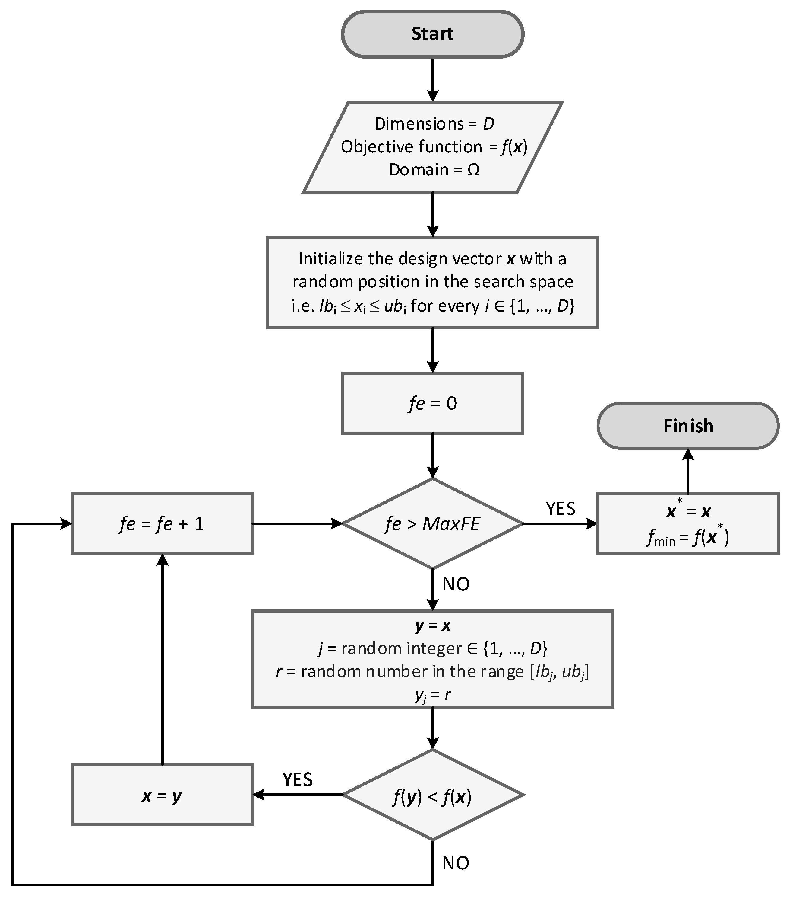
2.3. Pure Random Orthogonal Search
- Initialize x with a random position in the search space (feasible region Ω), i.e., lbi ≤ xi ≤ ubi for every i ∈ {1, …, D}
- Until a termination criterion is met, repeat the following:
- ○
- Set y = x
- ○
- Sample a random integer j ∈ {1, …, D}
- ○
- Sample a random number r in the range [lbj, ubj] using uniform distribution
- ○
- Set yj = r
- ○
- If f(y) < f(x) then move to the new position by setting x = y
- At the end, x holds the best-found position and f(x) is the best solution.
2.4. Methodology of the Study and Objective Functions Used
- Genetic algorithm (GA);
- Particle swarm optimization (PSO);
- Differential evolution (DE);
- Pure random search (PRS);
- Pure random orthogonal search (PROS).
2.5. Objective Functions
3. Results
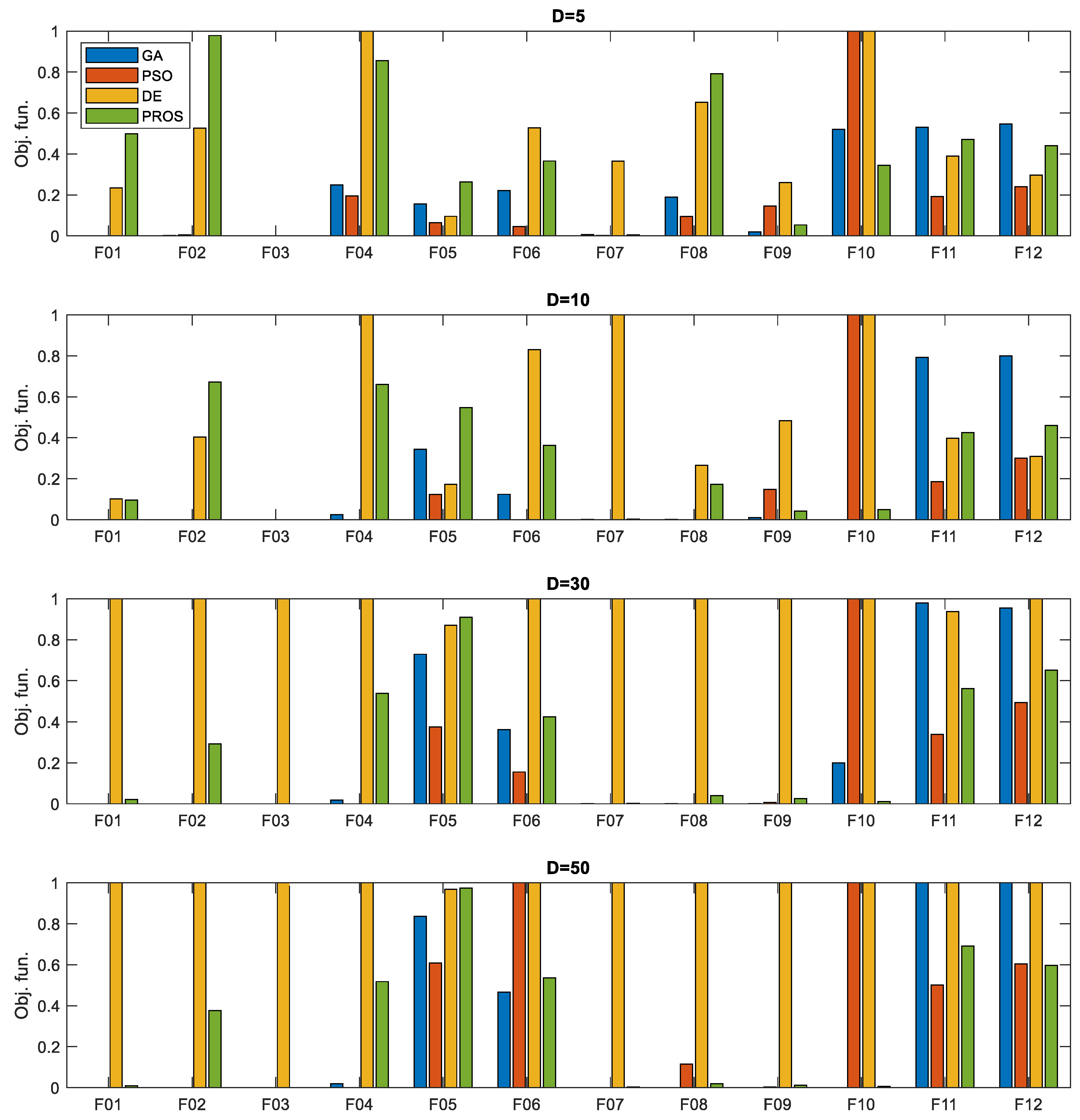
3.1. Objective Function Values
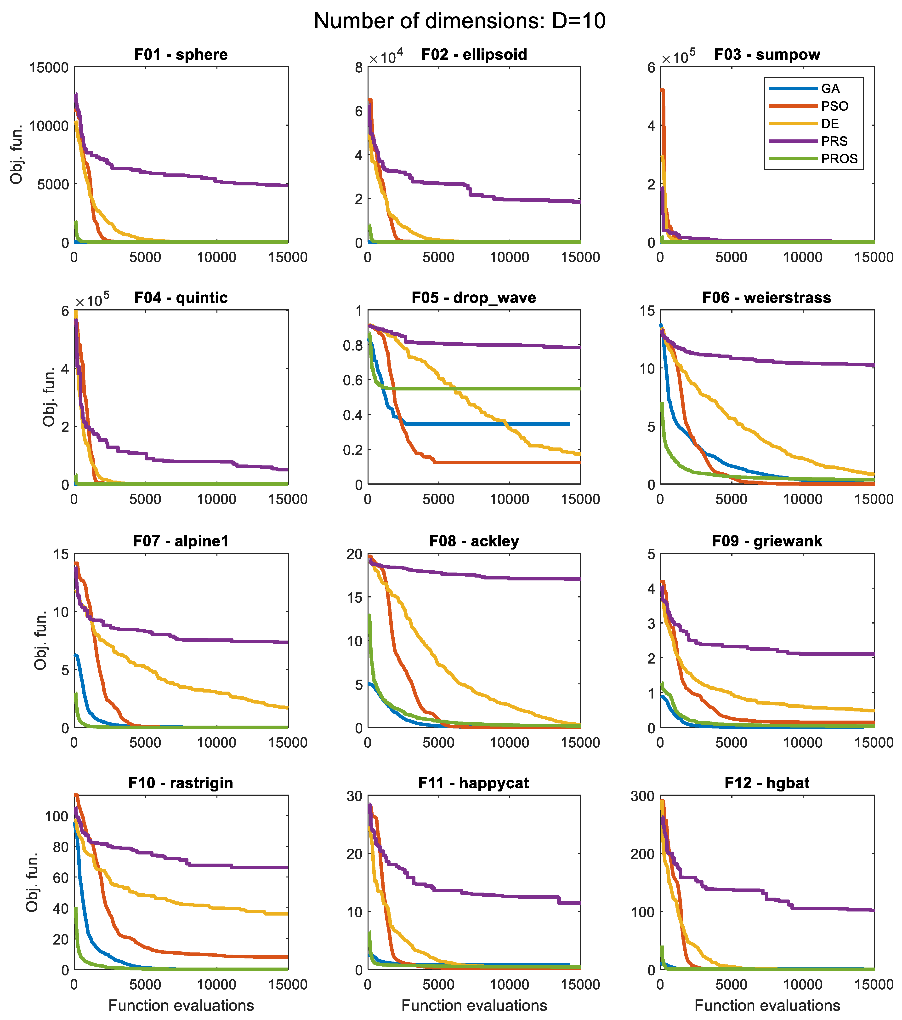
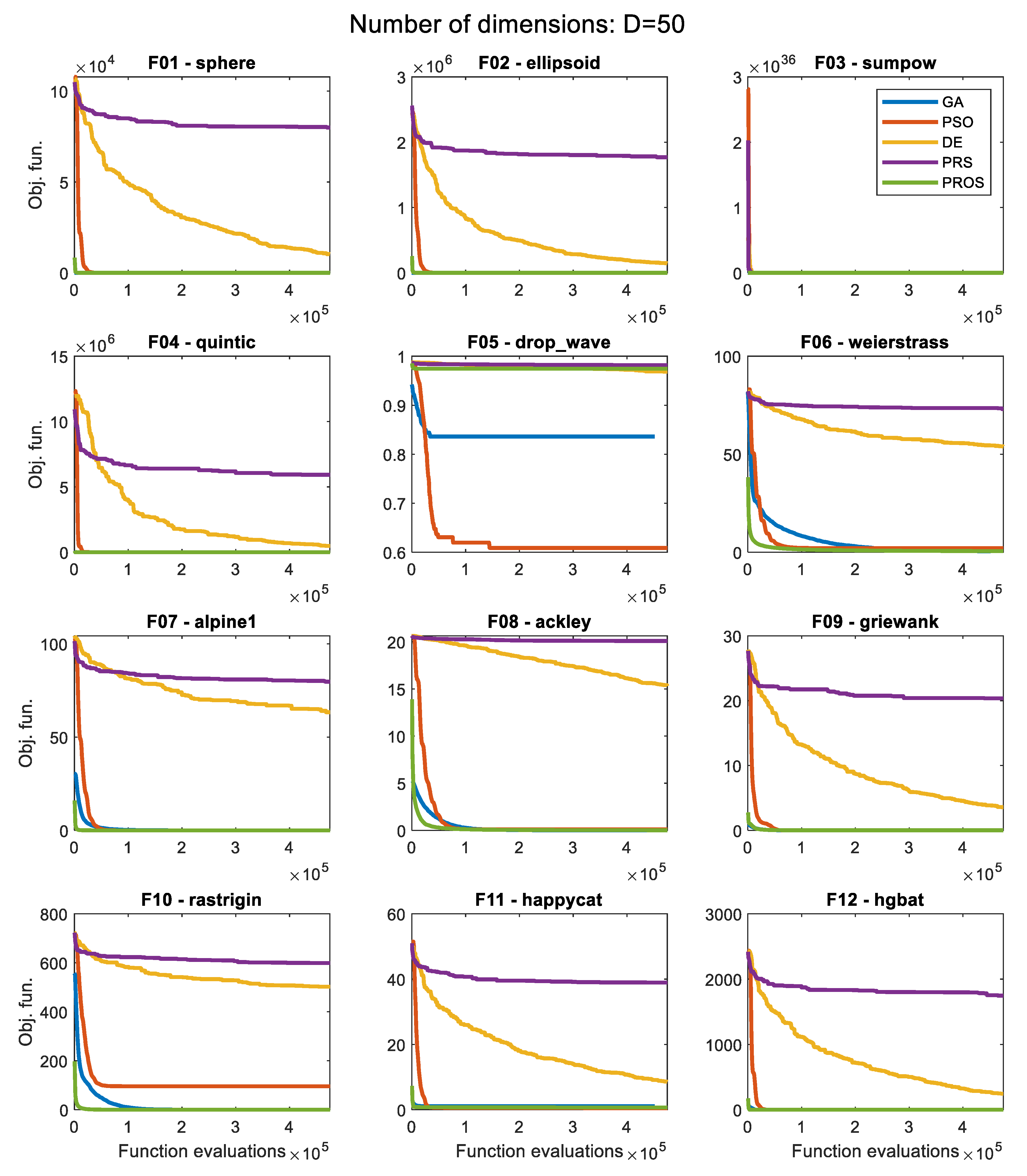
3.2. Convergence History for Each Algorithm
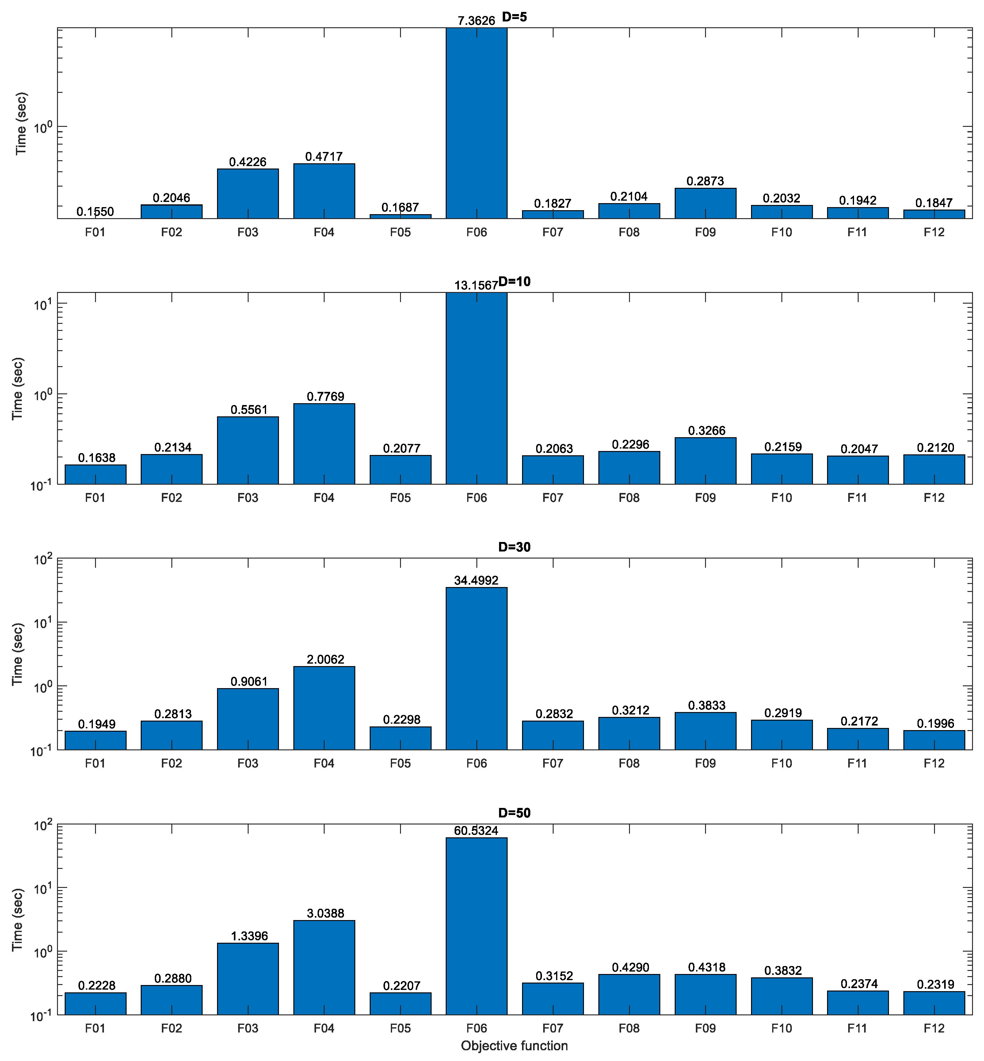
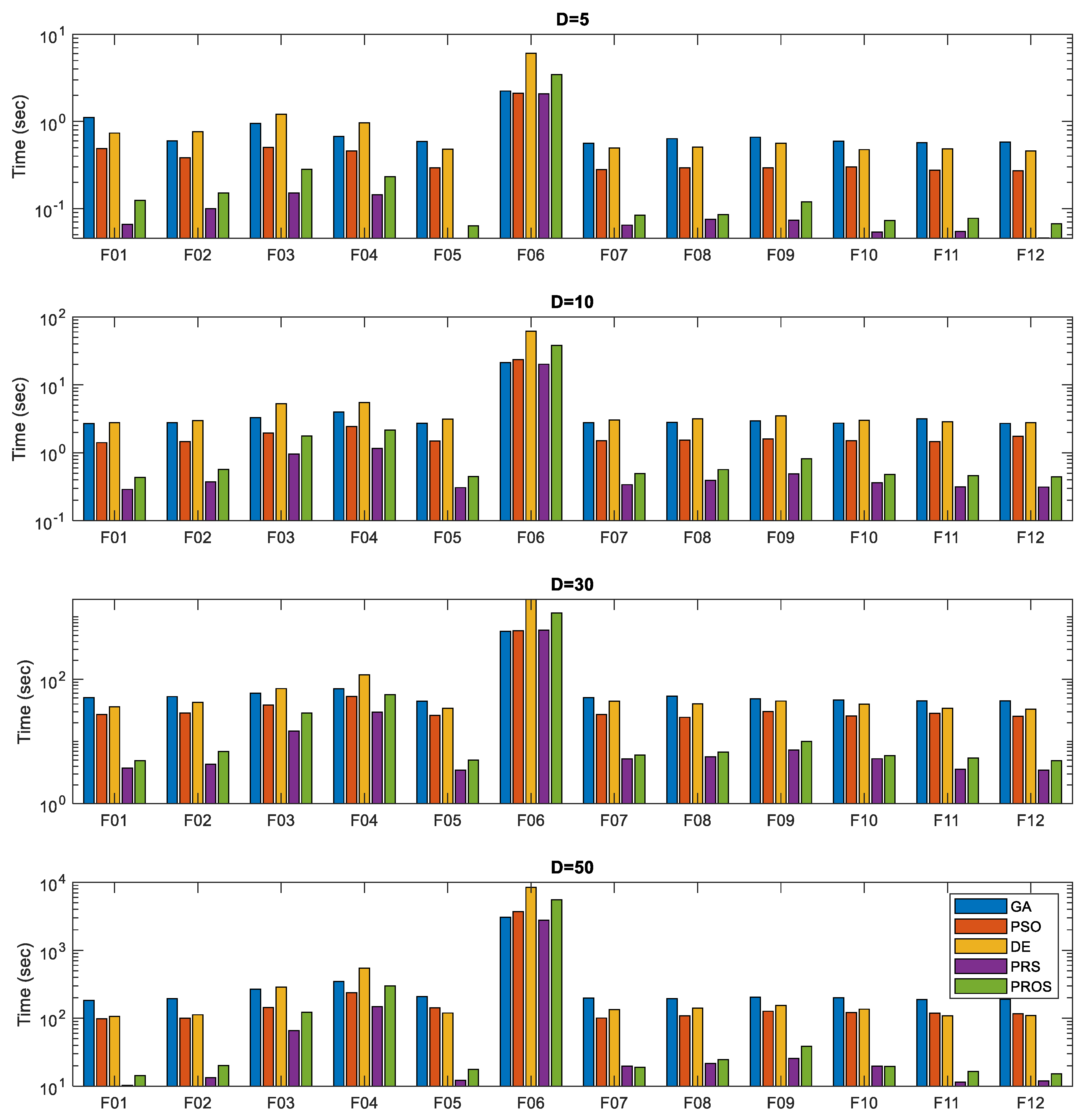
3.3. Computational Efficiency
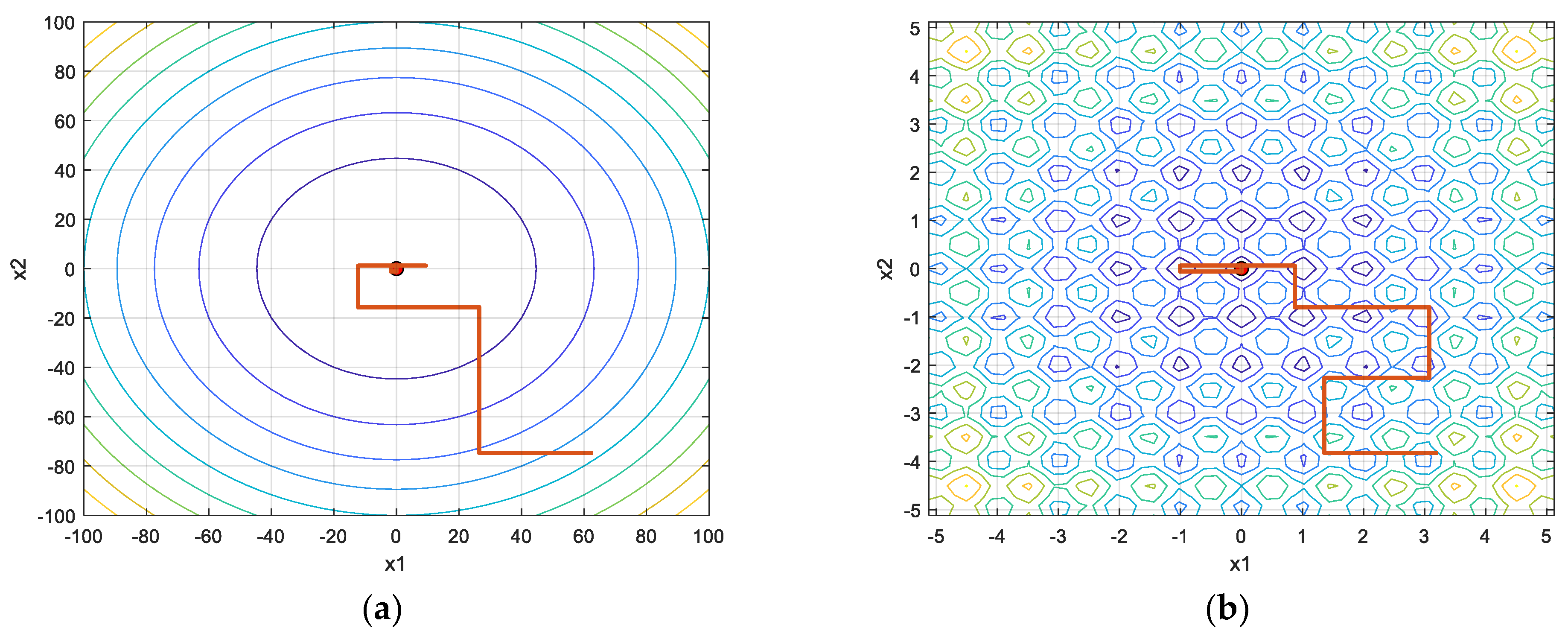
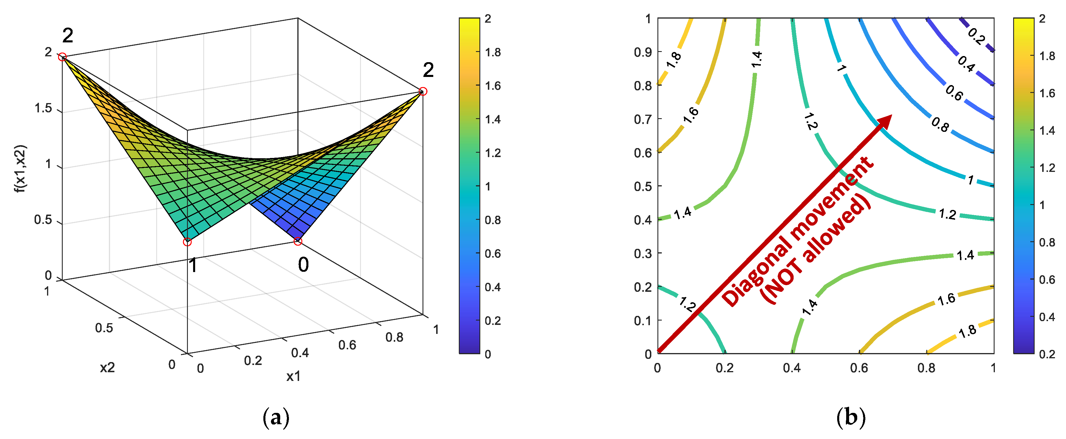
3.4. Conditions under Which PROS Can Be Trapped in A Local Optimum
- f(0, 0) = 1 (current solution)
- f(1, 0) = f(0, 1) = 2
- f(1, 1) = 0 (global minimum)
4. Discussion
4.1. Advantages and Drawbacks of PROS
4.2. PROS Applications
5. Conclusions
Future Directions
Author Contributions
Funding
Informed Consent Statement
Data Availability Statement
Conflicts of Interest
Appendix A. Nomenclature

| Acronym | Meaning |
|---|---|
| ACO | Ant colony optimization |
| DE | Differential evolution |
| GA | Genetic algorithm |
| HS | Harmony search |
| IOA | Improved optimization algorithm |
| NFL | No free lunch |
| OA | Optimization algorithm |
| PROS | Pure random orthogonal search |
| PRS | Pura random search |
| PSO | Particle swarm optimization |
| Symbol | Meaning |
|---|---|
| f(x) | Objective function |
| D | Dimensionality of the optimization problem (no. of dimensions) |
| Ω | Search space |
| D | A real coordinate space of dimension D |
| x or y | vector of decision variables |
| xi or yi | i-th decision variable, i-th element of the decision variables’ vector |
| lb/ub | Lower/upper bounds vector |
| lbi/ubi | Lower/upper bound for the decision variable xi |
| x* | Decision variables’ vector corresponding to the optimum solution |
| f(x*) | Optimum value of the function f |
| r | Random number |
| NP | Population size |
| MaxIter | Maximum number of iterations (or generations) |
| OFE | Maximum number of function evaluations |
| F | Differential weight of the DE algorithm |
| CR | Crossover probability of the DE algorithm |
Appendix B. Objective Functions Used in the Study


References
- Solorzano, G.; Plevris, V. Optimum Design of RC Footings with Genetic Algorithms According to ACI 318-19. Buildings 2020, 10, 110. [Google Scholar] [CrossRef]
- Goldberg, D.E. Genetic Algorithms in Search, Optimization and Machine Learning; Addison-Wesley Longman Publishing Co.: Boston, MA, USA, 1989. [Google Scholar]
- Holland, J. Adaptation in Natural and Artificial Systems; University of Michigan Press.: Ann Arbor, MI, USA, 1975. [Google Scholar]
- Plevris, V.; Karlaftis, N.D.; Lagaros, N.D. A Swarm Intelligence Approach for. Emergency Infrastructure Inspection Scheduling. In Sustainable and Resilient Critical Infrastructure Systems: Simulation, Modeling, and Intelligent Engineering; Gopalakrishnan, K., Peeta, S., Eds.; Springer: Heidelberg, Germany, 2010; pp. 201–230. [Google Scholar]
- Plevris, V.; Papadrakakis, M. A Hybrid. Particle Swarm—Gradient Algorithm for Global Structural Optimization. Comput. Aided Civ. Infrastruct. Eng. 2011, 26, 48–68. [Google Scholar] [CrossRef]
- Kennedy, J.; Eberhart, R. Particle Swarm Optimization. In Proceedings of the IEEE International Conference on Neural Networks, Piscataway, NJ, USA, 27 November–1 December 1995; pp. 1942–1948. [Google Scholar]
- Georgioudakis, M.; Plevris, V. A Combined Modal Correlation Criterion for Structural Damage Identification with Noisy Modal Data. Adv. Civ. Eng. 2018, 2018, 318067. [Google Scholar] [CrossRef]
- Georgioudakis, M.; Plevris, V. On the Performance of Differential Evolution Variants in Constrained Structural Optimization. Procedia Manuf. 2020, 44, 371–378. [Google Scholar] [CrossRef]
- Georgioudakis, M.; Plevris, V. A Comparative Study of Differential Evolution Variants in Constrained Structural Optimization. Front. Built Environ. 2020, 6, 1–14. [Google Scholar] [CrossRef]
- Storn, R.; Price, K. Differential Evolution—A Simple and Efficient Heuristic for Global Optimization over Continuous Spaces. J. Glob. Optim. 1997, 11, 341–359. [Google Scholar] [CrossRef]
- Dorigo, M.; Maniezzo, V.; Colorni, A. The Ant System: Optimization by a Colony of Cooperating Agents. IEEE Trans. Syst. Man Cybern. B. 1996, 26, 2941. [Google Scholar] [CrossRef] [PubMed] [Green Version]
- Geem, Z.W.; Kim, J.H.; Loganathan, G.V. A New Heuristic Optimization Algorithm: Harmony Search. SIMULATION 2001, 76, 60–68. [Google Scholar] [CrossRef]
- Gao, X.Z.; Govindasamy, V.; Xu, H.; Wang, X.; Zenger, K. Harmony Search Method: Theory and Applications. Comput. Intell. Neurosci. 2015, 2015, 258491. [Google Scholar] [CrossRef] [PubMed] [Green Version]
- Kirkpatrick, S.; Gelatt, C.D.; Vecchi, M.P. Optimization by Simulated Annealing. Science 1983, 220, 671–680. [Google Scholar] [CrossRef] [PubMed]
- Glover, F.; Taillard, E.; Taillard, E. A User’s Guide to Tabu Search. Ann. Oper. Res. 1993, 41, 1–28. [Google Scholar] [CrossRef]
- Wolpert, D.H.; Macready, W.G. No Free Lunch Theorems for Optimization. IEEE Trans. Evol. Comput. 1997, 1, 67–82. [Google Scholar] [CrossRef] [Green Version]
- Culberson, J.C. On the Futility of Blind. Search: An. Algorithmic View of “No Free Lunch”. Evol. Comput. 1998, 6, 109–127. [Google Scholar] [CrossRef] [PubMed]
- Ho, Y.C.; Pepyne, D.L. Simple Explanation of the No-Free-Lunch Theorem and Its Implications. J. Optim. Theory Appl. 2002, 115, 549–570. [Google Scholar] [CrossRef]
- Koziel, S.; Michalewicz, Z. Evolutionary Algorithms, Homomorphous Mappings, and Constrained Parameter Optimization. Evol. Comput. 1999, 7, 19–44. [Google Scholar] [CrossRef] [PubMed]
- Plevris, V. Innovative Computational Techniques for the Optimum Structural Design Considering Uncertainties; National Technical University of Athens: Athens, Greece, 2009; p. 312. [Google Scholar]
- Zabinsky, Z.B. Stochastic Adaptive Search for Global Optimization. In Nonconvex Optimization and Its Applications; Springer: New York, USA, 2003; ISBN 978-1-4419-9182-9. [Google Scholar]
- Spall, J.C. Introduction to Stochastic Search and Optimization: Estimation, Simulation, and Control; Wiley: Hoboken, NJ, USA, 2003; ISBN 9780471330523. [Google Scholar]
- Brooks, S.H. A Discussion of Random Methods for Seeking Maxima. Oper. Res. 1958, 6, 244–251. [Google Scholar] [CrossRef]
- Peng, J.-P.; Shi, D.-H. Improvement of Pure Random Search in Global Optimization. J. Shanghai Univ. 2000, 4, 92–95. [Google Scholar] [CrossRef]


| Step | xi/yi | Design Vector | Obj. Value | Notes | ||||
|---|---|---|---|---|---|---|---|---|
| 1 | 2 | 3 | 4 | 5 | ||||
| 1 | x1 | −34.32 | −5.13 | −58.68 | 1.29 | −22.26 | 5.15·103 | No improvement keep x1 for Step 2 (x2 = x1) |
| y1 (j = 4) | −34.32 | −5.13 | −58.68 | [14.73] | −22.26 | 5.36·103 | ||
| 2 | x2 | −34.32 | −5.13 | −58.68 | 1.29 | −22.26 | 5.15·103 | Improvement keep y2 for Step 3 (x3 = y2) |
| y2 (j = 3) | −34.32 | −5.13 | [35.52] | 1.29 | −22.26 | 2.96·103 | ||
| 3 | x3 | −34.32 | −5.13 | 35.52 | 1.29 | −22.26 | 2.96·103 | No improvement keep x3 for Step 4 (x4 = x3) |
| y3 (j = 5) | −34.32 | −5.13 | 35.52 | 1.29 | [−43.44] | 4.36·103 | ||
| 4 | x4 | −34.32 | −5.13 | 35.52 | 1.29 | −22.26 | 2.96·103 | Improvement keep y4 for Step 5 (x5=y4) |
| y4 (j = 1) | [11.97] | −5.13 | 35.52 | 1.29 | −22.26 | 1.93·103 | ||
| 5 | x5 | 11.97 | −5.13 | 35.52 | 1.29 | −22.26 | 1.93·103 | No improvement keep x5 for Step 6 (x6=x5) |
| y5 (j = 5) | 11.97 | −5.13 | 35.52 | 1.29 | [−88.95] | 9.35·103 | ||
| No of Dimensions, D | D = 5 | D = 10 | D = 30 | D = 50 |
|---|---|---|---|---|
| Population size NP NP = 10·D | 50 | 100 | 300 | 500 |
| Max. Generations/Iterations MaxIter MaxIter = 20·D − 50 | 50 | 150 | 550 | 950 |
| Max. Obj. function evaluations MaxFE MaxFE = NP·MaxIter | 2500 | 15,000 | 165,000 | 475,000 |
| ID | Name and Code Name | Search Range | Minimum | Properties |
|---|---|---|---|---|
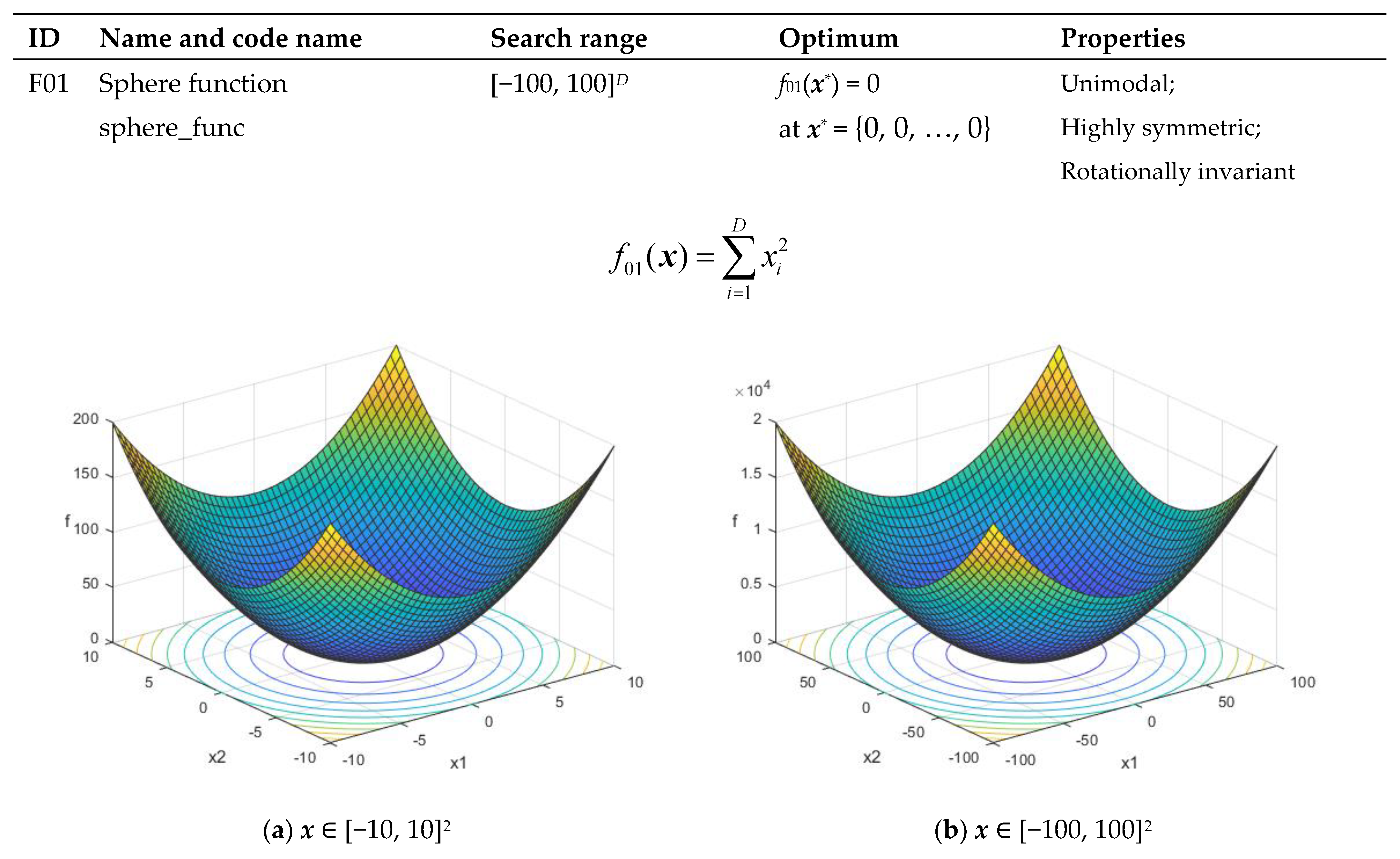
| F01 | Sphere function sphere_func | [−100, 100]D | f01(x*) = 0 at x* = {0, 0, …, 0} | Unimodal Highly symmetric, in particular rotationally invariant |
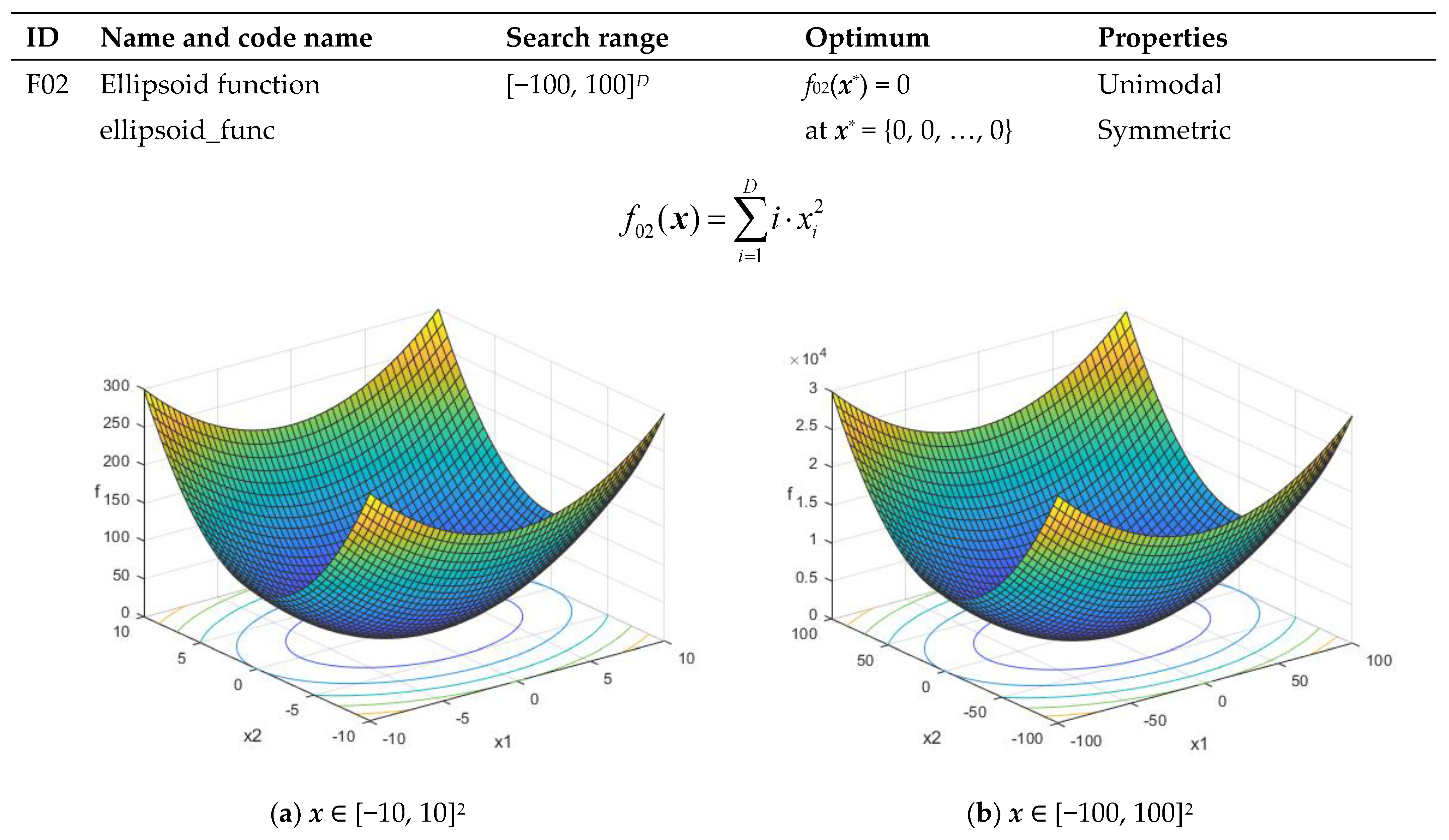
| F02 | Ellipsoid function ellipsoid_func | [−100, 100]D | f02(x*) = 0 at x* = {0, 0, …, 0} | Unimodal Symmetric |
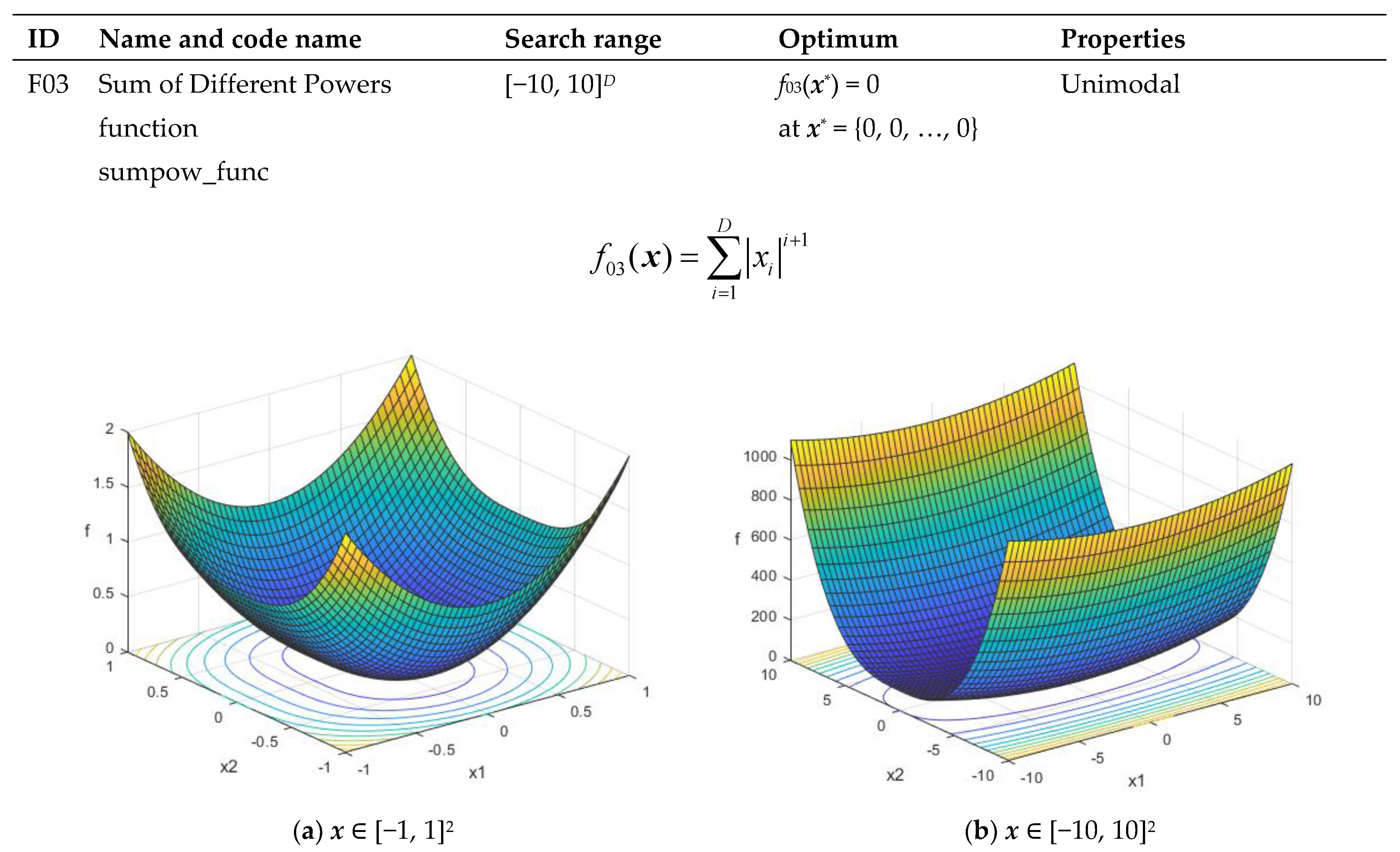
| F03 | Sum of Different Powers function sumpow_func | [−10, 10]D | f03(x*) = 0 at x* = {0, 0, …, 0} | Unimodal |
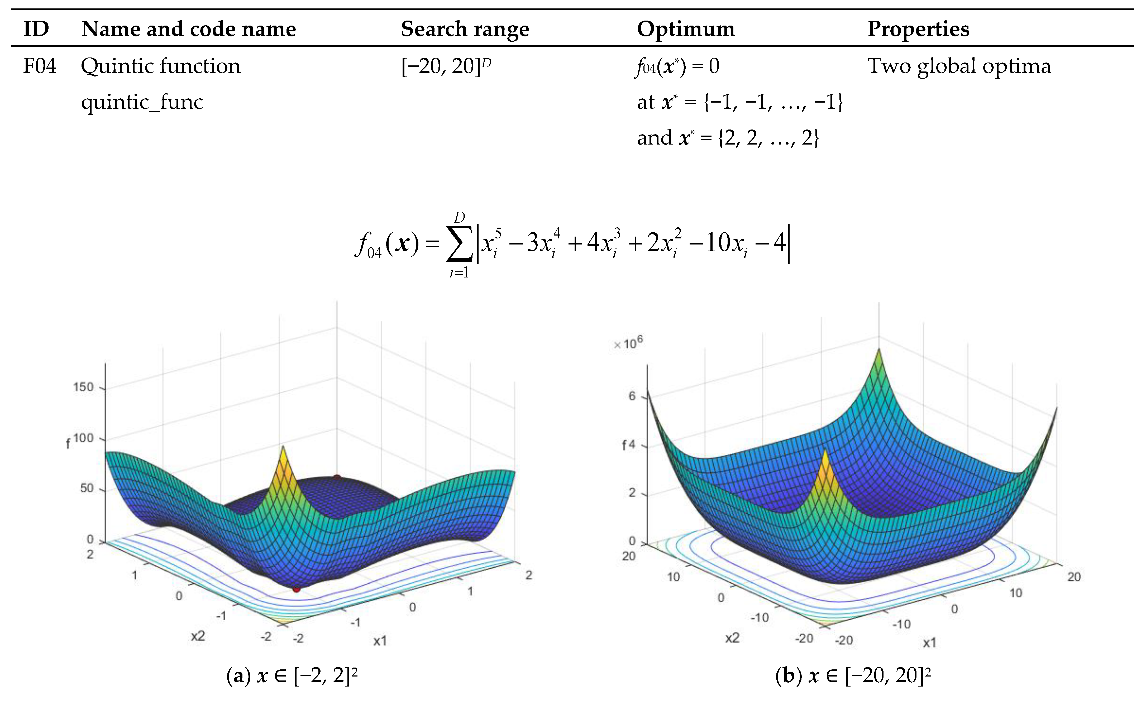
| F04 | Quintic function quintic_func | [−20, 20]D | f04(x*) = 0 at x* = {−1, -1, …, −1} or x* = {2, 2, …, 2} | Has two global optima |
| F05 | Drop-Wave function drop_wave_func | [−5.12, 5.12]D | f05(x*) = 0 at x* = {0, 0, …, 0} | Multi-modal Highly complex |
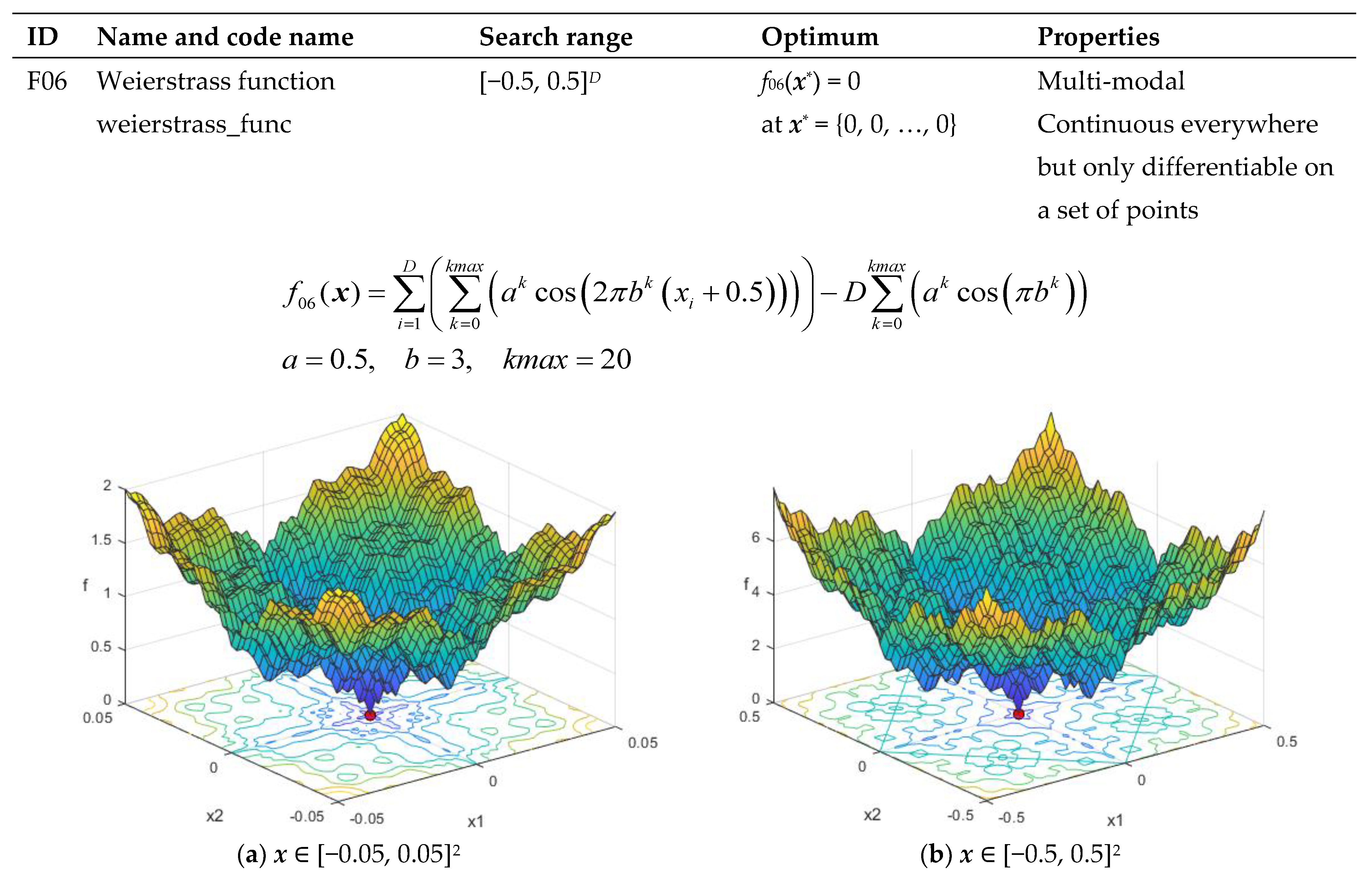
| F06 | Weierstrass function weierstrass_func | [−0.5, 0.5]D | f06(x*) = 0 at x* = {0, 0, …, 0} | Multi-modal Continuous everywhere but only differentiable on a set of points |
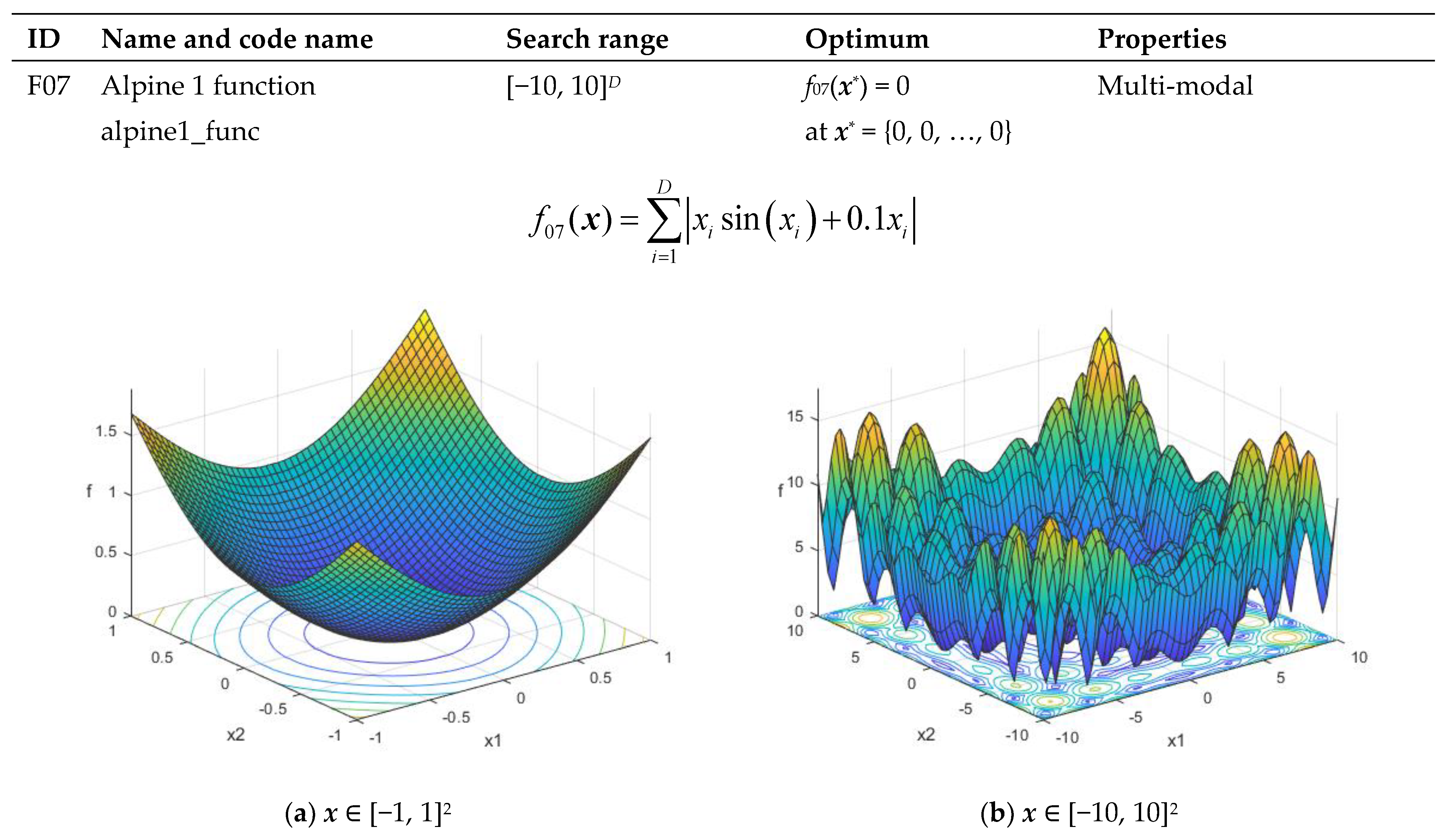
| F07 | Alpine 1 function alpine1_func | [−10, 10]D | f07(x*) = 0 at x* = {0, 0, …, 0} | Multi-modal |
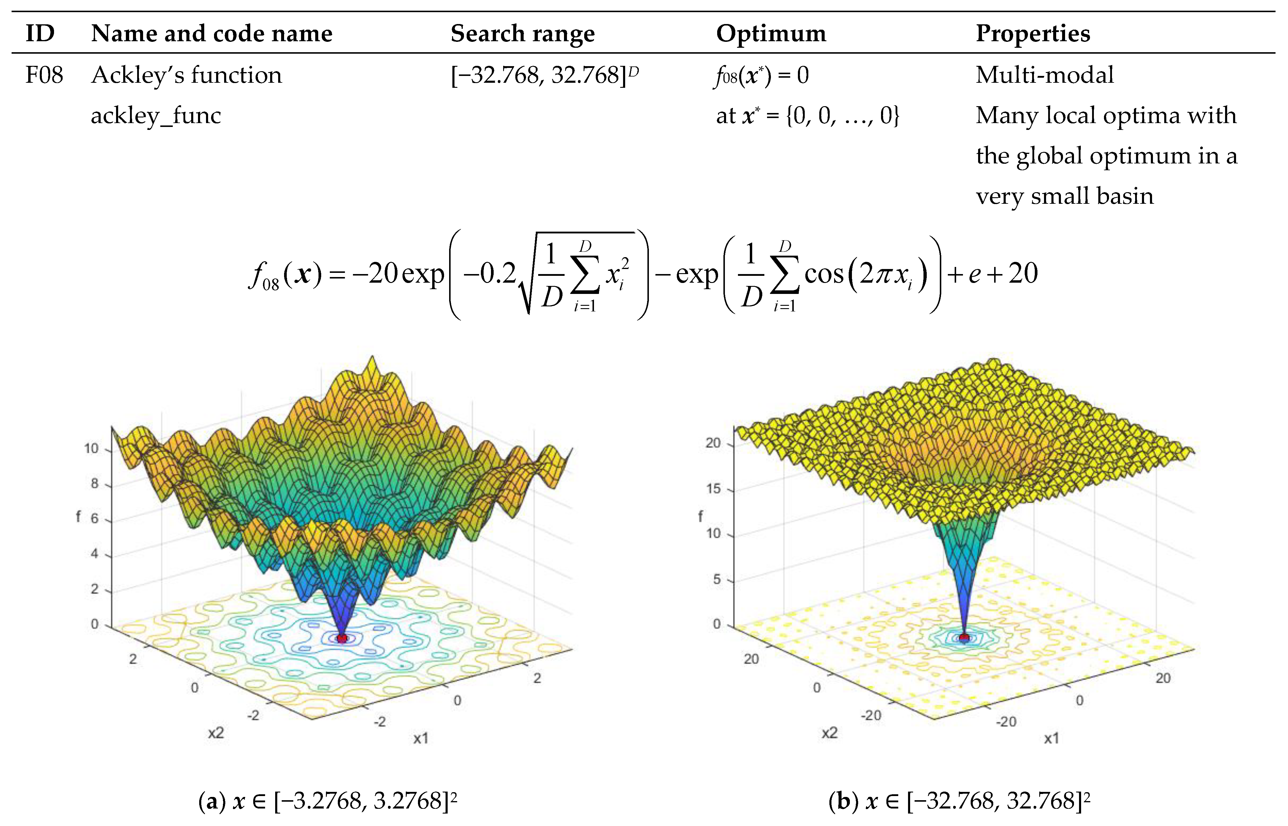
| F08 | Ackley’s function ackley_func | [−32.768, 32.768]D | f08(x*) = 0 at x* = {0, 0, …, 0} | Multi-modal Having many local optima with the global optima located in a very small basin |
| F09 | Griewank’s function griewank_func | [−100, 100]D | f09(x*) = 0 at x* = {0, 0, …, 0} | Multi-modal With many regularly distributed local optima |
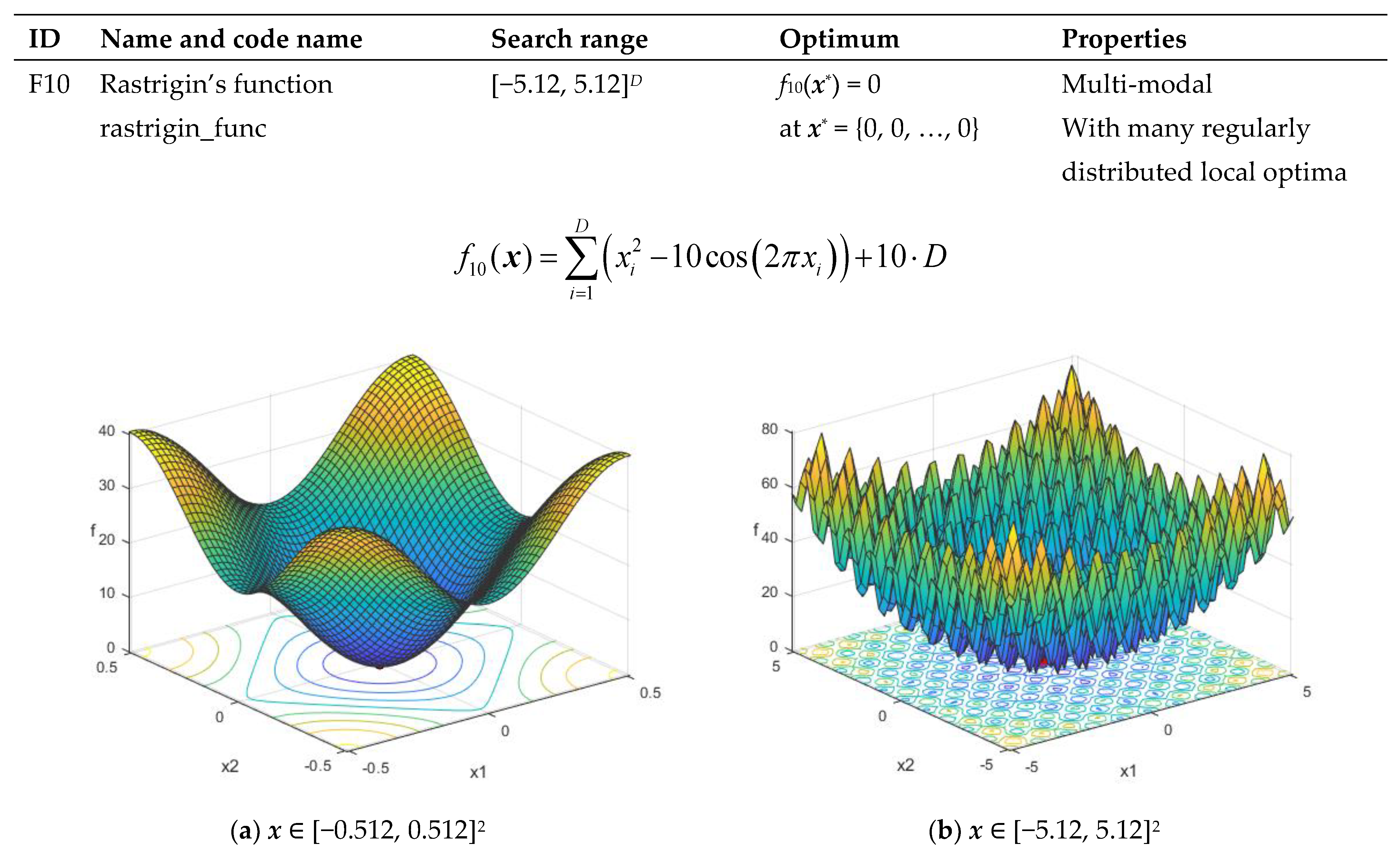
| F10 | Rastrigin’s function rastrigin_func | [−5.12, 5.12]D | f10(x*) = 0 at x* = {0, 0, …, 0} | Multi-modal With many regularly distributed local optima |
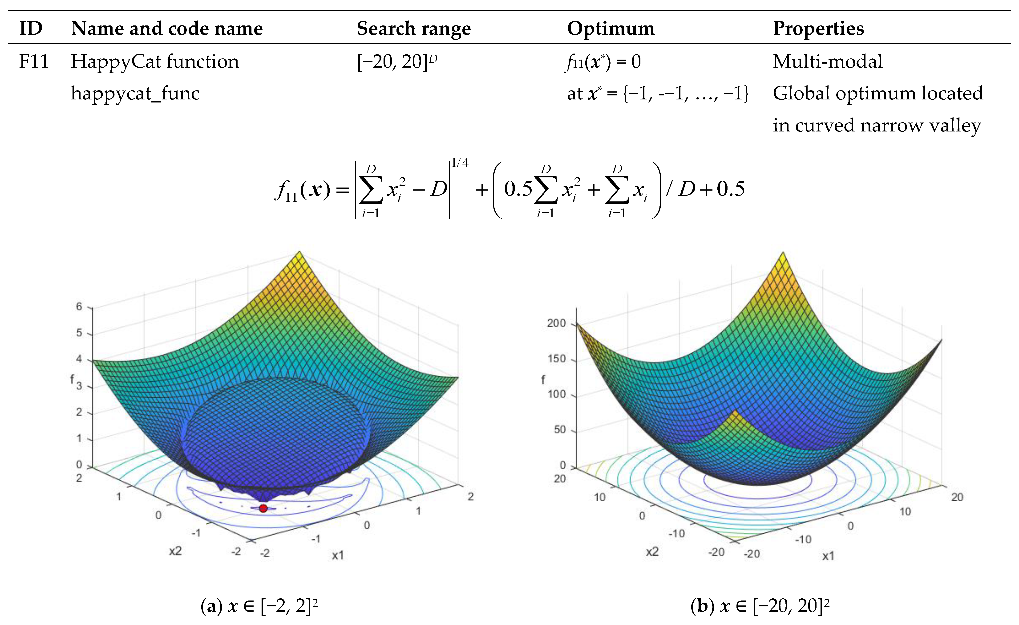
| F11 | HappyCat function happycat_func | [−20, 20]D | f11(x*) = 0 at x* = {−1, −1, …, −1} | Multi-modal Global optimum located in curved narrow valley |
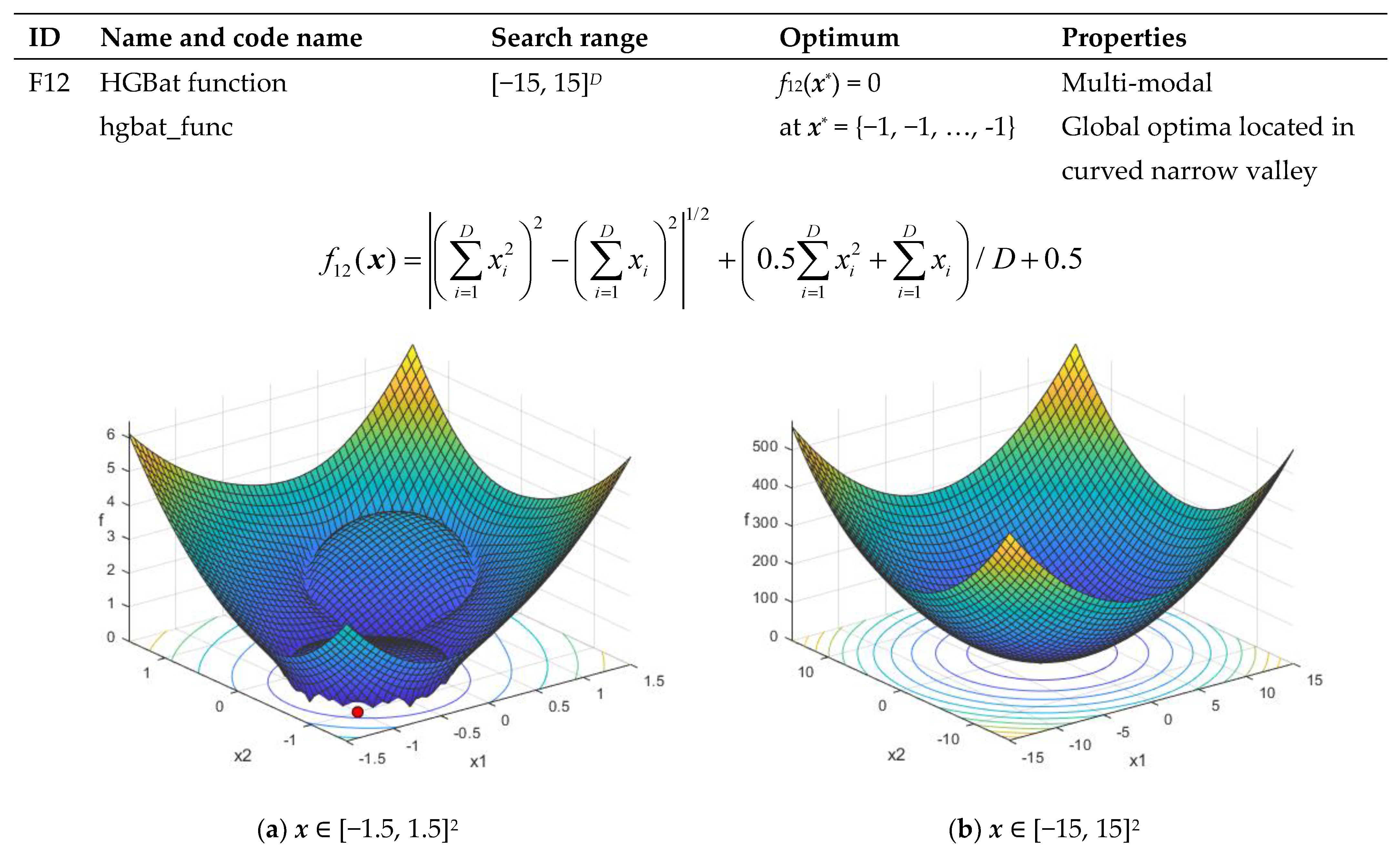
| F12 | HGBat function hgbat_func | [−15, 15]D | f12(x*) = 0 at x* = {−1, −1, …, −1} | Multi-modal Global optima located in curved narrow valley |
| ID | Function Name | D = 5 | D = 10 | D = 30 | D = 50 |
|---|---|---|---|---|---|
| F01 | Sphere | 4.99E-01 | 9.56E-02 | 2.17E-02 | 9.25E-03 |
| F02 | Ellipsoid | 9.78E-01 | 6.72E-01 | 2.92E-01 | 3.77E-01 |
| F03 | Sum of Dif. Powers | 8.07E-04 | 5.58E-05 | 5.35E-06 | 2.80E-06 |
| F04 | Quintic | 8.56E-01 | 6.61E-01 | 5.40E-01 | 5.18E-01 |
| F05 | Drop-Wave | 2.63E-01 | 5.48E-01 | 9.10E-01 | 9.74E-01 |
| F06 | Weierstrass | 3.66E-01 | 3.62E-01 | 4.25E-01 | 5.36E-01 |
| F07 | Alpine 1 | 4.99E-03 | 3.16E-03 | 2.36E-03 | 2.46E-03 |
| F08 | Ackley’s | 7.92E-01 | 1.72E-01 | 3.99E-02 | 1.87E-02 |
| F09 | Griewank’s | 5.34E-02 | 4.13E-02 | 2.51E-02 | 1.13E-02 |
| F10 | Rastrigin’s | 3.44E-01 | 4.94E-02 | 1.03E-02 | 5.74E-03 |
| F11 | HappyCat | 4.71E-01 | 4.25E-01 | 5.63E-01 | 6.92E-01 |
| F12 | HGBat | 4.40E-01 | 4.61E-01 | 6.51E-01 | 5.97E-01 |
| ID | Function Name | GA | PSO | DE | PRS | PROS |
|---|---|---|---|---|---|---|
| F01 | Sphere | 6.99E-04 | 9.04E-04 | 2.34E-01 | 8.30E+02 | 4.99E-01 |
| F02 | Ellipsoid | 2.12E-03 | 5.58E-03 | 5.26E-01 | 1.56E+03 | 9.78E-01 |
| F03 | Sum of Dif. Powers | 6.38E-06 | 1.85E-08 | 3.11E-05 | 2.15E+01 | 8.07E-04 |
| F04 | Quintic | 2.49E-01 | 1.95E-01 | 4.03E+00 | 2.33E+03 | 8.56E-01 |
| F05 | Drop-Wave | 1.56E-01 | 6.38E-02 | 9.55E-02 | 4.20E-01 | 2.63E-01 |
| F06 | Weierstrass | 2.21E-01 | 4.50E-02 | 5.27E-01 | 3.87E+00 | 3.66E-01 |
| F07 | Alpine 1 | 6.18E-03 | 2.39E-03 | 3.65E-01 | 1.93E+00 | 4.99E-03 |
| F08 | Ackley’s | 1.89E-01 | 9.54E-02 | 6.52E-01 | 1.19E+01 | 7.92E-01 |
| F09 | Griewank’s | 1.96E-02 | 1.46E-01 | 2.60E-01 | 1.00E+00 | 5.34E-02 |
| F10 | Rastrigin’s | 5.20E-01 | 3.70E+00 | 7.59E+00 | 2.08E+01 | 3.44E-01 |
| F11 | HappyCat | 5.31E-01 | 1.92E-01 | 3.89E-01 | 5.41E+00 | 4.71E-01 |
| F12 | HGBat | 5.46E-01 | 2.40E-01 | 2.97E-01 | 1.81E+01 | 4.40E-01 |
| ID | Function Name | GA | PSO | DE | PRS | PROS |
|---|---|---|---|---|---|---|
| F01 | Sphere | 6.93E-06 | 4.41E-11 | 1.02E-01 | 4.83E+03 | 9.56E-02 |
| F02 | Ellipsoid | 5.89E-05 | 3.83E-10 | 4.03E-01 | 1.83E+04 | 6.72E-01 |
| F03 | Sum of Dif. Powers | 4.22E-08 | 7.75E-23 | 1.57E-06 | 2.04E+03 | 5.58E-05 |
| F04 | Quintic | 2.42E-02 | 3.52E-05 | 1.04E+01 | 4.95E+04 | 6.61E-01 |
| F05 | Drop-Wave | 3.45E-01 | 1.24E-01 | 1.73E-01 | 7.85E-01 | 5.48E-01 |
| F06 | Weierstrass | 1.24E-01 | 9.90E-05 | 8.30E-01 | 1.03E+01 | 3.62E-01 |
| F07 | Alpine 1 | 1.10E-03 | 4.56E-07 | 1.68E+00 | 7.33E+00 | 3.16E-03 |
| F08 | Ackley’s | 1.94E-03 | 1.98E-06 | 2.66E-01 | 1.70E+01 | 1.72E-01 |
| F09 | Griewank’s | 1.06E-02 | 1.48E-01 | 4.83E-01 | 2.11E+00 | 4.13E-02 |
| F10 | Rastrigin’s | 1.96E-04 | 8.12E+00 | 3.61E+01 | 6.62E+01 | 4.94E-02 |
| F11 | HappyCat | 7.92E-01 | 1.86E-01 | 3.98E-01 | 1.14E+01 | 4.25E-01 |
| F12 | HGBat | 8.00E-01 | 3.00E-01 | 3.09E-01 | 1.02E+02 | 4.61E-01 |
| ID | Function Name | GA | PSO | DE | PRS | PROS |
|---|---|---|---|---|---|---|
| F01 | Sphere | 7.50E-07 | 4.03E-26 | 3.70E+02 | 3.58E+04 | 2.17E-02 |
| F02 | Ellipsoid | 2.25E-05 | 1.15E-24 | 2.80E+03 | 4.57E+05 | 2.92E-01 |
| F03 | Sum of Dif. Powers | 1.50E-12 | 1.54E-52 | 3.50E+03 | 2.46E+15 | 5.35E-06 |
| F04 | Quintic | 1.80E-02 | 4.43E-14 | 2.73E+03 | 1.92E+06 | 5.40E-01 |
| F05 | Drop-Wave | 7.29E-01 | 3.76E-01 | 8.71E-01 | 9.63E-01 | 9.10E-01 |
| F06 | Weierstrass | 3.63E-01 | 1.55E-01 | 2.06E+01 | 4.06E+01 | 4.25E-01 |
| F07 | Alpine 1 | 3.37E-04 | 7.42E-15 | 2.54E+01 | 3.86E+01 | 2.36E-03 |
| F08 | Ackley’s | 6.89E-04 | 4.37E-14 | 6.08E+00 | 1.94E+01 | 3.99E-02 |
| F09 | Griewank’s | 1.23E-03 | 6.39E-03 | 1.07E+00 | 1.01E+01 | 2.51E-02 |
| F10 | Rastrigin’s | 1.99E-01 | 4.56E+01 | 2.34E+02 | 3.14E+02 | 1.03E-02 |
| F11 | HappyCat | 9.79E-01 | 3.39E-01 | 9.38E-01 | 2.88E+01 | 5.63E-01 |
| F12 | HGBat | 9.55E-01 | 4.95E-01 | 7.12E+00 | 8.32E+02 | 6.51E-01 |
| ID | Function Name | GA | PSO | DE | PRS | PROS |
|---|---|---|---|---|---|---|
| F01 | Sphere | 1.03E-06 | 2.04E-34 | 1.03E+04 | 8.00E+04 | 9.25E-03 |
| F02 | Ellipsoid | 3.50E-05 | 1.19E-32 | 1.46E+05 | 1.77E+06 | 3.77E-01 |
| F03 | Sum of Dif. Powers | 8.98E-13 | 3.65E-60 | 6.01E+14 | 1.50E+30 | 2.80E-06 |
| F04 | Quintic | 1.87E-02 | 3.42E-15 | 4.79E+05 | 5.92E+06 | 5.18E-01 |
| F05 | Drop-Wave | 8.36E-01 | 6.09E-01 | 9.68E-01 | 9.82E-01 | 9.74E-01 |
| F06 | Weierstrass | 4.66E-01 | 2.08E+00 | 5.39E+01 | 7.30E+01 | 5.36E-01 |
| F07 | Alpine 1 | 3.84E-04 | 1.99E-14 | 6.33E+01 | 7.97E+01 | 2.46E-03 |
| F08 | Ackley’s | 5.50E-04 | 1.16E-01 | 1.53E+01 | 2.01E+01 | 1.87E-02 |
| F09 | Griewank’s | 4.44E-08 | 2.47E-03 | 3.59E+00 | 2.04E+01 | 1.13E-02 |
| F10 | Rastrigin’s | 1.25E-04 | 9.60E+01 | 5.02E+02 | 5.99E+02 | 5.74E-03 |
| F11 | HappyCat | 1.08E+00 | 5.01E-01 | 8.57E+00 | 3.89E+01 | 6.92E-01 |
| F12 | HGBat | 1.06E+00 | 6.04E-01 | 2.46E+02 | 1.75E+03 | 5.97E-01 |
Publisher’s Note: MDPI stays neutral with regard to jurisdictional claims in published maps and institutional affiliations. |
© 2021 by the authors. Licensee MDPI, Basel, Switzerland. This article is an open access article distributed under the terms and conditions of the Creative Commons Attribution (CC BY) license (https://creativecommons.org/licenses/by/4.0/).
Share and Cite
Plevris, V.; Bakas, N.P.; Solorzano, G. Pure Random Orthogonal Search (PROS): A Plain and Elegant Parameterless Algorithm for Global Optimization. Appl. Sci. 2021, 11, 5053. https://doi.org/10.3390/app11115053
Plevris V, Bakas NP, Solorzano G. Pure Random Orthogonal Search (PROS): A Plain and Elegant Parameterless Algorithm for Global Optimization. Applied Sciences. 2021; 11(11):5053. https://doi.org/10.3390/app11115053
Chicago/Turabian StylePlevris, Vagelis, Nikolaos P. Bakas, and German Solorzano. 2021. "Pure Random Orthogonal Search (PROS): A Plain and Elegant Parameterless Algorithm for Global Optimization" Applied Sciences 11, no. 11: 5053. https://doi.org/10.3390/app11115053
APA StylePlevris, V., Bakas, N. P., & Solorzano, G. (2021). Pure Random Orthogonal Search (PROS): A Plain and Elegant Parameterless Algorithm for Global Optimization. Applied Sciences, 11(11), 5053. https://doi.org/10.3390/app11115053