Article

Conjoining Wymore’s Systems Theoretic Framework and the DEVS Modeling Formalism: Toward Scientific Foundations for MBSE

1
Grado Department of Industrial and Systems Engineering, Virginia Polytechnic Institute and State University, Blacksburg, VA 24061, USA
2
RTSync Corp., Chandler, AZ 85226, USA
*
Author to whom correspondence should be addressed.
Appl. Sci. 2021, 11(11), 4936; https://doi.org/10.3390/app11114936
Submission received: 8 March 2021 / Revised: 17 May 2021 / Accepted: 19 May 2021 / Published: 27 May 2021

Abstract

:

Featured Application

This research contributes toward the theoretical foundations of model-based systems engineering (MBSE) through combining the mathematical, system theoretic framework for MBSE developed by A. Wayne Wymore with the computational systems theory of Discrete Event System Specification (DEVS). This research leads to internally consistent, holistic modeling and simulation-based systems engineering and a science to MBSE.

Abstract

The objective of this research article is to re-introduce some of the concepts provided by A. Wayne Wymore in his mathematical theory of Model-Based Systems Engineering, discuss why his framework might have not been adopted, and define a potential path to modernize the framework for practical application in the digital age. The dense mathematical theory has never been converted to a practical form. We propose a path to modernization by creating a metamodel of Wymore’s mathematical theory of MBSE. This enables explaining the concepts in simple to understand terms and shows the internal consistency provided by the theory. Furthermore, the metamodel allows for conversion of the theory into software application, for which we show some initial results that open the research to the art of the possible. In recognition of limitation of the theory, we make the case for a merger of the theoretical framework with the enhanced formalism of Discrete Event System Specification (DEVS). This will establish a path toward the scientific foundations for MBSE to enable future implementations of the complementary pairing and their empirical results.

1. Introduction

Recent thrust in the systems engineering (SE) community has been toward the use of models to perform SE activities [1]. This change comes from a desired conversion away from document-based SE (DBSE) to model-based SE (MBSE) to leverage potential improvements such as traceability through authoritative sources of truth [2]. However, a recent survey presented several obstacles to the adoption of MBSE in practice [3], alluding, among others, to conceptual misalignment. In fact, models from the leading MBSE language, the Systems Modeling Language (SysML), have been shown to have multiple interpretations [4]. We argue that these barriers may be symptoms of a lack of a theoretical foundation for MBSE. While current practices of MBSE provide digital representations of the system model through descriptively linking elements within and related to the system, they lack a formal underlying foundation, such as could be provided through mathematical theory [5]. This is in contrast to more traditional engineering disciplines, such as mechanical engineering or electrical engineering, where modeling tools leverage formal mathematical foundations (e.g., finite element analysis and computational fluid dynamics). We contend that such foundations are necessary to enable a science-informed approach to MBSE.
Several efforts in that direction were initiated several decades ago, including von Bertalanffy’s General Systems Theory [6], Weiner’s Cybernetics [7], Mesarovic and Takahara’s general [8] and abstract systems [9] theories, Zeigler’s computational systems theory [10], and Wymore’s Mathematical Theory of Systems Engineering [11]; after which no other contribution at such scale has been completed. The SE community did not ground its practice upon such foundation at the time and is reclaiming now a new wave of research to unveil the theoretical foundations of SE [12,13,14,15,16,17]. This vision aligns with that of the International Council on Systems Engineering (INCOSE), which has called for SE to “be grounded in more rigorous foundations of mathematics” [1].
From a historical perspective, coining the term MBSE has been credited to A. Wayne Wymore [18,19] through his mathematical framework for system design that he comprehensively referred to as the Tricotyledon Theory of System Design (T3SD) [20]; a tricotyledon refers to a triad of leaf-shaped spaces. In Wymore’s words, he created T3SD “to provide the system theoretic foundations necessary to the study and practice of systems engineering” and “to explicate mathematical system theory as the basis for the development of models and designs of large-scale, complex systems consisting of personnel, machines, and software” [20]. Conceptually, T3SD defines a mathematically guided process of engineering systems through reliance on formal mappings between designs that have increasing technology dependence. The term “tricotyledon” originates in the distinctive three cotyledon leaf configurations of the Buildability space, the Functionality space, and the Implementability space. The subset of buildable designs that formally map to the subset of functional designs constitutes the space of implementable designs. For simplicity, a visualization of the conceptualization of Wymore’s T3SD is shown in Figure 1.
Wymore defined three levels of system designs in T3SD: the functional system design (FSD), the buildable system design (BSD), and the implementable system design (ISD). The mapping between the design elaborations that comes with increasing technology dependences allows for verification, validation, and evaluation between functionality and buildability of the system.
Wymore believed that it would take decades or generations for his research to receive its due appreciation [21]. Upon Wymore’s passing, evidence of influence on the SE community can be found in the literature [22]. In further review of the literature, some provide reference to T3SD [23,24,25,26,27]. With Wymore being “often credited with introducing a mathematical foundation for MBSE” [23], it should be assumed that the literature would provide significant usage, enhancement, and reference to his research. However, as one author states, Wymore’s framework is “difficult to translate” [28] and “hard to follow such that only mathematicians are able to read it” [19]. While certainly dense in mathematical equations, theory, and proofs, this should not preclude exploration of T3SD from the SE community for usage as a foundation for modern MBSE and its necessary evolution. However, we agree on the lack of digestibility of T3SD in its current form. Therefore, with this research article we aim to bring awareness to T3SD and provide insights into its modernization for practical application within the rapidly progressing digital paradigm for engineering of systems.
We propose a simplified variant of Wymore’s framework, and thereby reclaim its merit. SysML is used to capture key variables and their relationships in the form of a metamodel. Study of T3SD led to extraction of equations from [20] and creation of the metamodel. From the extracted equations and metamodel, we define possible practical applications, discuss some limitations of T3SD. We then define a path to enhance T3SD through merger with an alternate formalism. A natural choice for such a formalism is the Discrete Event System Specification (DEVS).
DEVS is an evolutionary steppingstone from the overlooked T3SD that is grounded in practice and well-studied. Recent research suggests that DEVS provides a path to simulation basis for MBSE [5]. Furthermore, INCOSE has established a joint working group with the International Association for Engineering Modeling and Simulation (NAFEMS) directed toward reconciliation of systems modeling (MBSE) and simulation (DEVS) [29]. Also, the basis for the merger of T3SD and DEVS is well-founded as the “DEVS formalism was defined as a specification for a subclass of Wymore systems” [10], which is a reference to Wymore original research in his 1967 publication of the Mathematical Theory of SE [11]. We will discuss the possible future applications of this complementary pairing as well as areas of Wymore’s research that require further understanding prior to defining its applicability within the current digital paradigm. We then conclude that this research provides a foundational contribution toward defining a science to modeling the engineering of systems (i.e., science of MBSE) through a yet to be developed theory. This lays the foundation for future implementation of the complementary pairing that will involve empirical results.

2. Methods

Wymore’s mathematical theory of “Model-Based Systems Engineering” book provides the most extensive treatment of T3SD [20]. Wymore was a proponent of Unicode [30], which was intended to serve as a universal language for machines. As such, his work is often challenging to interpret. Therefore, in this article, we attempt to balance between Wymore’s use of Unicode and readability. From his book [20], equations consisting of vectors were extracted. Some vector equations were deemed to be applications of the theory rather than core to the theory. These are not included in this research article. The included vector equations were deemed to be “core equations” to Wymore’s theory. For simplification and communication purposes, we have created two of our own equations. No information has been lost in the creation of the two equations. The equations increase the digestibility of T3SD and, as such, their representations are used in the metamodel. This is captured in a metamodel of T3SD. For our purposes, a metamodel is defined as a model of a model. In this case, the full T3SD is a model of the engineering of systems and our metamodel is a concise abstraction of T3SD; meaning that we do not claim to capture every relationship in T3SD. Capturing every relationship in T3SD is outside of the scope of this research article. Furthermore, we do not define a formal ontological construct in this article; and, as such, we distinguish the term metamodel from the term ontology, which are often used interchangeably.
For creating our metamodel, SysML’s implementation in Cameo System Modeler ® from Dassault Systems (Boston, MA, USA) [31] was used. Blocks were chosen to represent elements of T3SD. Relationships between elements of T3SD are represented as a directed relationship. For an explanation of how to read the T3SD model, refer to Figure 2. Flashlight, Light Source, and Human are considered elements, which are represented as blocks. This is read as Light Source is a component of a Flashlight and the Human provides input to the Flashlight.
To aid in following our research in this article, we provide the SysML activity diagram in Figure 3. The activity diagram introduces various elements of T3SD as high-level terms. These terms will be formally defined later in this article. Although not specified in the diagram, iteration is possible at every stage returning to earlier activities. Other renditions of the process that Wymore may have had in mind might be imaginable.

3. Results

In this section, we show how the metamodel was constructed with description of each subset of relationships. This is followed by showing how T3SD is related to DEVS; thus, enabling a convergence between the two.

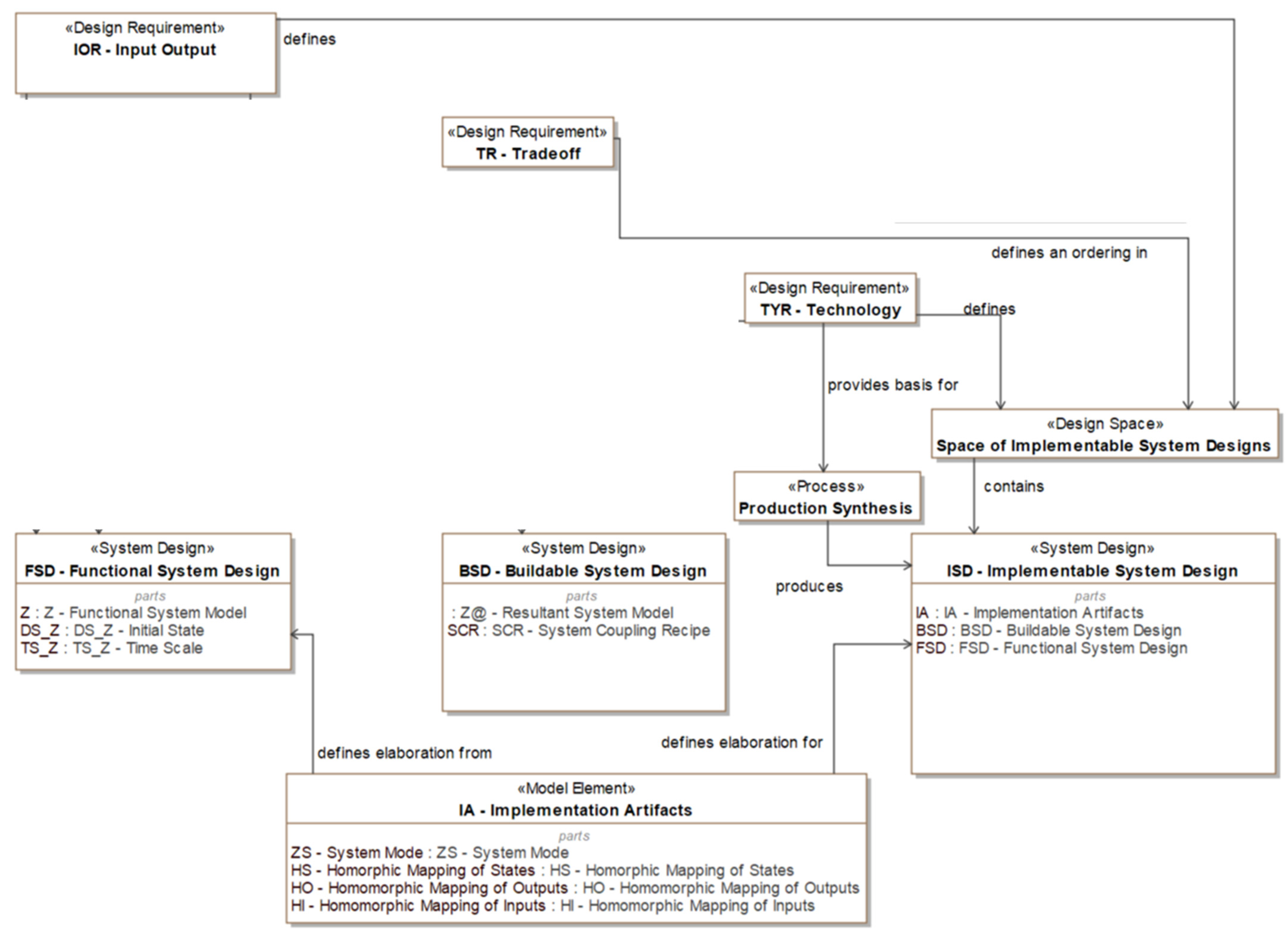
3.1. A Systematic Description of the T3SD Metamodel

In this section, subsets of the metamodel are deconstructed to show how the overall metamodel was constructed. This allows for an understanding of different relationships in the metamodel, starting with the first subset in Figure 4). The full metamodel is shown in Appendix A in Figure A1; supporting equations are shown in Appendix B; and crosswalk between the equations and metamodel are shown in Appendix C Table A1. The remainder of this section deconstructs the metamodel for clarity of interpretation.
We begin by showing the first subset of the metamodel in Figure 4. The items in this subset of the metamodel form the basis for the title and contents of the first four subsections of Section 3.1. We follow this by reviewing the System Design Requirement (SDR). This is followed by descriptions of the three spaces (cotyledons) that Wymore used to define the functional, buildable, and implementable spaces of system designs as well as their distinctions and relationships. To conclude this section, we provide an illustration of T3SD using the example of a flashlight to articulate the concepts.

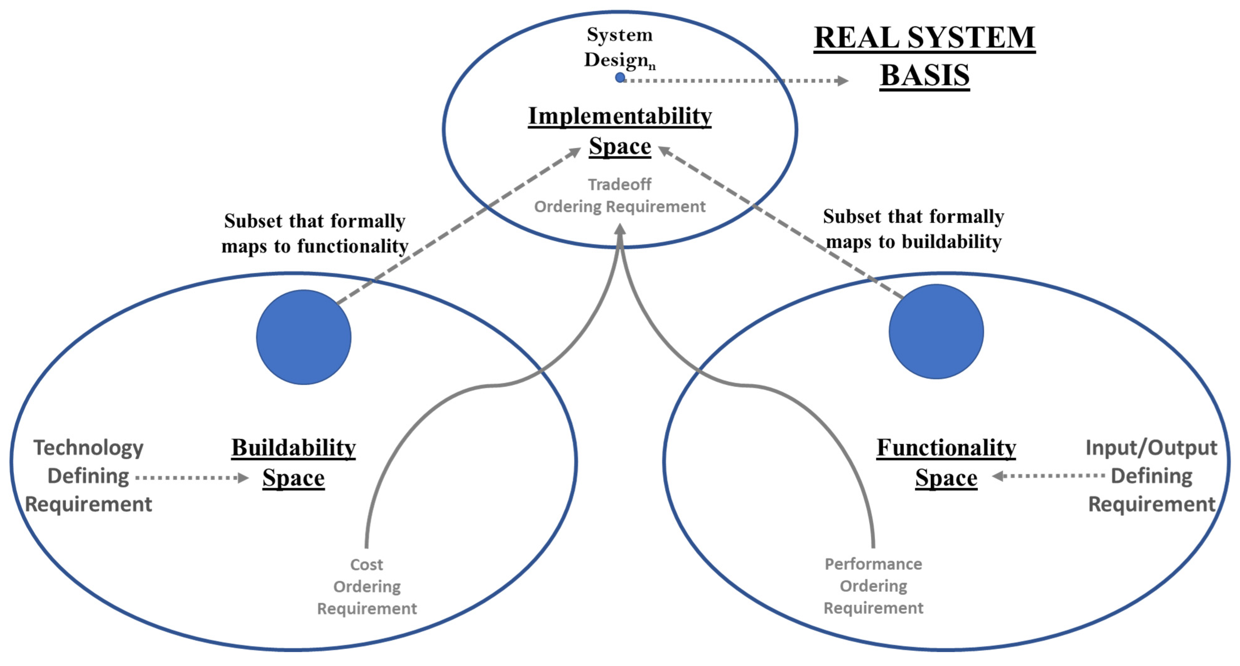
3.1.1. The Problem Space (Wymore’s System Design Requirement)

Within T3SD, Wymore defined the SDR as the set of Input Output Requirement (IOR), System Test Requirement (STR), Cost Requirement (CR), Performance Requirement (PR), Tradeoff Requirement (TR), and Technology Requirement (TYR). The STR references the CR, TR, PR, and IOR for tests conducted for the system design. The SDR are discussed in more detail in the following sections from the perspectives of functionality, buildability, and implementability.

3.1.2. The Functionality Perspective (Wymore’s Functional Cotyledon)

The IOR describes the required input to output transformations that the system must execute, yielding in this way a space of functional system designs. A Functional System Design (FSD), which results from conducting a System Functional Analysis, describes the functionality provided by a system. The FSD is independent of technology, is defined prior to decomposition and allocation of system level requirements, and is the most abstract representation of the system in T3SD. It is modeled as the combination of a state machine that we refer to as the Functional System Model (Z), an Initial State (DSZ), and the Time Scale (TSZ).
Selection of a specific FSD within the space of functional system designs is driven by the PR. Whereas the IOR defines a space of functional system designs, PR defines an order in such space. The PR is used as a mechanism to order the alternative FSDs according to preferred consistency with satisfaction of the IOR [20]. This does not preclude from conducting tests on more elaborate system designs; within T3SD, system tests are conducted on the ISD, which contains the FSD.
These relationships are shown as a subset of the metamodel in Figure 5.

3.1.3. The Buildability Perspective (Wymore’s Buildability Cotyledon)

The TYR describes the specification of the set of the physical (tangible -hardware, software, etc.) components that are available to build the system. In this sense, this type of requirements, which can be interpreted as predefined technologies that must be used, is inconsistent with common guidelines for writing good requirements, since they unnecessarily enforce design solutions [32,33,34]. Nevertheless, we include this type of requirements here to faithfully represent T3SD. TYR yield a space of buildable system designs. A Buildable System Design (BSD) represents a system formed by the interconnection of physical components and, therefore, is technology dependent. The behavior of the BSD emerges from the way in which its components are inter-connected to each other and allocate the external inputs and outputs, modeled by the system coupling recipe (SCR). This is Wymore’s concept of system coupling, defined as “a specification of the system models to be coupled as components and a specification of which output ports of which components are to be connected to which input ports of which components” [35]. Wymore also introduced the concept of closure under coupling [35,36,37]. Closure under coupling requires that the set of system models must be closed under the operation of constructing the system resulting from a system coupling recipe, called the resultant (Z@) of the recipe. This is a formal representation of the principal by which system models are able to be hierarchically constructed through coupling of component system models. Wymore distinguished between a “component“ of a system and a “subsystem,” where the latter refers to a subset of its state space that is not necessarily associated with any component in a coupling recipe. Consistency of Wymore’s basis on the Moore state machine [38] enables measured elaboration through homomorphic relationship from the resultant of a BSD (Z@) to the system model (Z) of the functional design. However, a key aspect in Wymore’s framework is that a BSD may or may not implement the functionality in FSD. This is because, as presented, the space of BSDs is only shaped by TYR, with no influence of IOR.
Selection of a specific BSD within the space of BSDs is driven by the CR. Whereas the TYR defines a space of BSDs, CR defines an order in such space. In Wymore’s words, CR is used as a “means of which any two [alternative BSDs] can be compared consistently” [20]. These are not limited to traditional financial cost, but may also include acquisition timing restrictions [39]. As with PR, this does not preclude from conducting tests on more elaborate system designs; within T3SD, system tests are conducted on the ISD, which contains the BSD.
These relationships are shown as a subset of the metamodel in Figure 6.

3.1.4. The Implementability Perspective (Wymore’s Implementability Cotyledon)

The union of IOR and TYR yields the space of implementable system designs (ISDs). This implies that the space of the implementable system designs is the intersection of the space of FSDs with the space of BSDs. In essence, an ISD is a BSD that can exhibit the behavior of a given FSD. The space of ISDs captures BSDs that implement the behavior of FSDs, which then undergo production synthesis to serve as the basis for the real system [35]. Whereas not every FSD will be buildable and not every BSD will provide the required functionality, the ISD guarantees both conditions (which are necessary to produce a real system): a buildable system (BSD) that has at least one system mode (ZS) with a homomorphic relationship to the functional system model (Z) of the FSD. This is captured in the metamodel through the implementation artifacts (IA) that, in addition to ZS, include a homomorphic mapping of states (HS), homomorphic mapping of input (HI), and homomorphic mapping of output (HO).
Selection of a specific ISD within the space of ISDs is driven by the TR. Whereas IOR and TYR define a space of ISDs, TR defines an order in such space. In Wymore’s words, TR is used as a “means of which any two [alternative ISDs] can be compared consistently with respect to a trade-off between the performance [PR] and cost [CR] requirements” [20]. As indicated in [39], the required tradeoff may provide a preference toward performance over cost, a preference toward cost over performance, or equal preference between performance and cost.
These relationships are shown as a subset of the metamodel in Figure 7.

3.1.5. Illustration of T3SD Concepts

For the practical illustration of the flashlight, let us consider a set of system requirements such that the system must provide at least certain level of light when receiving a dedicated command, Pon, to do so and must provide no light when receiving another dedicated command, Poff. We denote the no light condition and the minimum level of light by L0 and L>=2, respectively. Furthermore, we define L0 and L>=2 to be mutually exclusive, as are the pair Poff and Pon. The IOR define that, when Pon, the system provides L>1, and when Poff, the system provides L0. Furthermore, L0 and L>1 are defined as different values of a single output port and Poff and Pon as different values of a single input port.
The IOR defines the space of FSDs shown in Figure 8, where each state machine represents one possible solution in the functionality space. Wymore selected the Moore state machine [38] as the basis for the FSDs. For simplicity, we have considered six different FSD’s, denoted by FSDi, with i = 1,…,6. L3 denotes a level of light intensity higher than L2, L0 denotes a level of light intensity lower than L1 but higher than no light, LS denotes an intermittent light, and P denotes a single type of command. FSD1, FSD2, and FSD3 meet the IOR and hence belong to the space of FSD, whereas FSD4, FSD5, and FSD6 do not meet the IOR and hence do not belong to the space of FSD defined by IOR.
Consider now two PR, such that more light intensity is preferred to less, and uniform lighting is preferred to non-uniform lighting, and the latter is preferred over the former. These requirements set an order on the space of FSDs such that F S D 3 F S D 2 F S D 1 .
The corresponding illustration of the functional perspective of an engineered flashlight is shown in Figure 8.
Continuing with the flashlight example, let us consider a set of TYR such that the available technologies include three different light sources (denoted by Z1, Z2, and Z3, providing intensity levels L1, L2, and L3, respectively), one sounding alarm (denoted by Z4), and two control systems (denoted by Z5, Z6, and Z7, providing one, two, and three input values, respectively). These TYR give form to a space of BSDs formed by any meaningful combination of Z1,…,Z7. For simplicity, we only show five of such BSDs, which we denote by BSDi, with i = 1,…,5, and depict in Figure 8, where each pair of box with internal blocks and state machine represent one solution in the buildability space. While those solutions present behaviors, note that these are irrelevant in the buildability space and only TYR are considered. This is why BSD3, representing a sound alarm, is considered an acceptable solution. Furthermore, in a real-world application, the state space of a coupled model is the cross-product of the state sets of the components. Rather than show the state space, we show the minimization of the result (Z@) of each BSD for simplification of this illustration. The minimization of a system is its homomorphic image with the least number of states [37].
Consider now two CR such that lower development cost is preferred over higher development cost. These requirements set an order on the space of BSDs such that BSD1 > BSD2 > BSD4 > BSD3 > BSD5, where > denotes preferred to.
The corresponding illustration of the buildability perspective of an engineered flashlight is shown in Figure 9.
Continuing with the flashlight example, we find the intersection of the space of FSD and the space of BSD by evaluating the functionality of the systems in the space of BSDs and buildability of the systems in the space of FSDs. These are shown in Figure 10, where each pair block diagram/state machine represent one possible solution inside or outside of the implementability space. For real-world application, a homomorphism is a mapping from a subset of the cross-product of the components states of BSD to the target system (FSD) where the subset can be shown to be a subsystem (i.e., closed under state transitions). For simplification of this illustration, we show only a representation of the homomorphic mapping of the resultant (Z@) of the BSD to the FSD. It can be seen that BSD1, BSD2, and BSD3 do not present any mode of behavior that is homomorphic to solutions in the space of FSD, since the inputs of BSD1 and BSD3 and the outputs of the three of them are different from those required by the IOR. Therefore, BSD1 and BSD2 do not belong to the space of ISDs. Similarly, it can also be seen that FSD2 does not have a corresponding BSD. Therefore, FSD2 does not belong to the space of ISDs.
The functionality of BSD4 is, however, directly mappable to FSD1, and hence BSD4 belongs to the space of ISDs; and we denote it by ISD1. BSD5 has a mode of behavior that is mappable to FSD1 (when Pon2 is unused) and a mode of behavior that is mappable to FSD3 (when Pon1 is unused). Both solutions belong to the space of ISDs and we denote them by ISD2 and ISD3, respectively. Furthermore, because no solution in the BSD implements a mode of operation that is homomorphic to the behavior of FSD2, FSD2 stays outside of the space of ISDs.
Consider now TR that (simplistically stated) lower cost takes precedence over higher light. (A detailed description of different types of TR can be found in [40].) This requirement sets an order on the space of ISDs such that ISD1 > ISD2 = ISD3, where > denotes preferred to and = denotes indifference.
The corresponding illustration of the implementability perspective of an engineered flashlight is shown in Figure 10.

3.2. A Brief Review of DEVS and Associated Formalism

At this point, we provide a short overview of the DEVS formalism and its relation to general systems theory. The DEVS formalism, introduced in 1976 [41], serves as the basis for the Theory of Modeling and Simulation. A brief summary of the set theoretic formulation appears in Appendix D. Please refer to [10] for a recent, complete presentation of these concepts.

3.2.1. Overview of the DEVS

The DEVS formalism formalizes what a model is, what it must contain, and what it does not contain (for instance, experimentation and simulation control parameters are not contained in the model). Moreover, DEVS is universal and unique for discrete-event system models. Any system that accepts events as inputs over time and generates events as outputs over time is equivalent to a DEVS model. With DEVS, a model of a large system can be decomposed into smaller component models with couplings between them. The DEVS formalism defines two kinds of models: (i) atomic models that represent the basic models providing specifications for the dynamics of a system components, and (ii) coupled models that describe how to couple several component models (which can be atomic or coupled models) together to form a new model. This hierarchical construction stems from the proof that a coupled model behaves like an atomic model due to DEVS formalism’s closure under coupling which is strongly linked to systems being well-defined [36].
An atomic DEVS model can be considered as an automaton with a set of states and transition functions allowing the state to change when an event occurs or due to the passage of time. When no events occur, the state of the atomic model is updated by the internal transition function upon expiration of its lifetime. When an external event occurs, the atomic model intercepts it and changes its state by applying its external transition function. The lifetime of a state is determined by a time advance function. Each state change can produce output messages via the output function. Examples of such DEVS models, including atomic and coupled models in operation, can be found in [10].
An abstract simulator algorithm is associated with the DEVS formalism in order to execute the structure of a model to generate its behavior. This technology-free abstract simulator standard enables DEVS models to be simulated on multiple different execution platforms, including those on desktops (for development) and those on high-performance platforms (such as Clusters or High Performance Computers).
The DEVS formalism includes continuous, parallel, coupled, networked, and Markov modeling (probabilistic) [10]. The DEVS formalism has been demonstrated for SoS application [42,43]. Furthermore, the basis of DEVS on Wymore’s system definition suggests that the foundation for the pairing of DEVS with T3SD is already present [10].
The Iterative System Specification and its relation to the DEVS formalism enables defining various continuous, discrete, and hybrid models for which simulations are possible [10]. The concept of system coupling has been proven within DEVS to allow for coupling of both discrete and continuous systems through closure under coupling [36]. The Iterative Specification of DEVS also allows for use of morphisms to maintain measured consistency and deviation throughout the specification of the various system models [10].

3.2.2. Hierarchy of System Specifications and Associated Morphisms

The essence of modeling lies in establishing relations between pairs of system descriptions. Such relations pertain to a variety of situations exemplified by:
  • the validity of representation of a real system by a model,
  • the validity of a simplified model relative to a more complex model from which it is derived,
  • the validity of a system description at one level of specification relative to a system description at a higher or lower level, and
  • the correctness of a simulator with respect to a model that it is simulating.
Table 1 identifies seven basic levels of system specification forming a Systems Specification Hierarchy. The fourth column gives an example of a system specification at each level applied to a flashlight. At each level we know some important things about a system that we did not know at lower levels.
At the lowest level, the source level identifies a portion of the real world that we wish to model and the means by which we are going to observe it.
At the next level, the data level is a data base of measurements and observations made for the source system. When we get to Level 2, we have the ability to recreate this data using a more compact representation, such as a formula. Since typically, there are many formulas or other means to generate the same data, the generative level, or particular means or formula we have settled on, constitutes knowledge we did not have at the data system level. When people talk about models in the context of simulation studies, they are usually referring to the concepts identified at this level. That is, to them a model means a program to generate data.
At the last level, that of Networked Systems, we have a very specific kind of generative system. In other words, we know how to generate the data observed at Level 1 in a more specific manner in terms of component systems that are interconnected together and whose interaction accounts for the observations made. When people talk about systems, they are often referring to this level of knowledge. They think of reality as being made up of interacting parts so that the whole is a function of its parts. Although some people use the term ‘subsystems’ for these parts, we call them component systems within the DEVS formalism (and reserve the term subsystem for another meaning in this paper).
The System Specification Hierarchy is a useful starting point for system modeling since it provides a unified perspective on what are usually considered to be distinct concepts. From this perspective, there are only three basic kinds of problems dealing with systems and they involve moving between the levels of system knowledge. Figure 11 identifies basic levels of system specification forming a Systems Specification Hierarchy with arrows directing their associated morphisms. At each level we can know, or can specify, important things about a system that are not knowable, or specifiable, at lower levels.
Based on the arrangement of system levels shown in Figure 11, we distinguish between vertical and horizontal relations. A horizontal relation is called an association mapping. It takes a system at one level of specification and elaborates it or abstracts it at another level of specification. The motion in the direction from Level 6 (Network of Systems) to Level 0 (I/O Frame) formally represents the process by which a simulator generates the behavior of a model. While the vertical association of specifications is straightforward, the association in the horizontal direction from Level 0 (I/O Frame) to Level 6 (Network of Systems) is much less so because travel in this direction requires acquisition or specification of additional system knowledge. In other words, it is possible that many structures exhibit the same behavior. Thus, recovering a unique structure from a given behavior is not possible except in special circumstances, called justifying conditions. For a complete description of the justifying conditions enabling structural inference, see [41].
The general concepts of homomorphism and isomorphism relate to the vertical relations which relate system models at the same level of specification. Corresponding to each of the various levels at which a system may be known, described, or specified, is a relation appropriate to a pair of systems specified at that level. We call such a relation a preservation relation or system morphism because it establishes a correspondence between a pair of systems whereby features of the one system are preserved in the other.
For system morphisms, we take the point of view illustrated in Figure 12, where S represents a “big“ system and S‘ a “little“ system. For example, S could be a base model and S‘ a lumped model. Accordingly, the basic orientation is that a part of the behavior of the big system S is mapped on the little system S‘ and the morphism is taken to be surjective. System S‘ therefore represents part of the system S with a certain degree of accuracy (Figure 12a). On the other hand, we also may employ mappings which go in the other direction, i.e., from the small system to the big one and we have an injective mapping. This ensures that all the behavior of small S‘ is covered by big S (Figure 12b).
Morphisms appropriate to each level of system specification are defined such that higher level morphisms imply lower level morphisms. This means that a morphism which preserves the structural features of one system in another system at one level, also preserves its features at all lower levels. For example, consider a morphism between systems at the I/O System Level in Figure 10. This morphism must be defined so that it induces a morphism at the I/O Function Level between the associated systems at that level and indeed, between the associated systems at the I/O Relation and I/O Frame levels. For a complete description of the morphisms defined for each adjacent pair of levels, see [10].

3.3. Pairing T3SD with DEVS

In this section, we provide the case for merging the T3SD framework with the DEVS formalism. To do this, we must first acknowledge some limitations of the current formalism of the T3SD framework within the context of modern SE.
The first is that T3SD is discrete and deterministic modeling. While all systems can be modeled as discrete systems, the margin of error may increase to the point of becoming a useless representation of the real system [10]. Additionally, modeling SE aspects such as the “ilities” (e.g., reliability and availability) and risk, in need of theoretical foundations for SE [17], requires the adoption of stochastic, probabilistic models. While Wymore’s original Mathematical Theory of SE was based on differential equations [11]; he had been working to add continuous systems to his MBSE framework [21] and recognized the need for event-based system specification [personal communication between Wymore and Zeigler, co-author in this paper]. Unfortunately, such research was left unfinished. Therefore, to modernize T3SD in this area, formalism must be added such as to enable continuous, probabilistic, and discrete event modeling.
The second is a potential limitation in T3SD admitted by Wymore. The explicit use of Wymore’s system coupling recipe (SCR) may have some limits; “in the SCR where the components in [the vector of systems to be coupled] are not discrete, the coupling function may not exist” [20]. Therefore, we suggest that for T3SD to be modernized, the concept of coupling must be further explored.
The third is that of simulation. It is not unfounded that Wymore’s T3SD be paired with simulation. Wymore’s use of system coupling has been credited for providing the system theoretic foundations for modeling and simulation [44]. Although this was in reference to Wymore’s first book on the Mathematical Theory of SE [11], simulation of the Moore-based state machines of T3SD is straight forward. Furthermore, Wymore acknowledged the necessity of a minimal system model in his article on reuse of commercial-off-the-shelf (COTS) parts, which “will make is easier to prove equivalence and therefore facilitate reuse” [37]. The concept of a minimal system model is foundational to the Theory of Modeling and Simulation [41]. Additionally, some initial capability of modeling and simulation support for T3SD was provided in Chapter 12 of [45]. Furthermore, simulation based on Wymore’s Mathematical Theory of SE [11] was formalized as the General Systems Theory (GEST) Simulator in [46] and later implemented in [47]. The modelling world view of GEST is based on the axiomatic system theory of Wymore [11,48]. GEST is a model and simulation specification language, therefore a GEST program is highly descriptive and acts as a documentation (for communication among humans) as well as a specification (for man-machine communication) [47]. This provides further evidence toward justification of convergence of Wymore’s T3SD with simulation.
As stated previously, the modernization needs of T3SD include formalisms beyond discrete and deterministic, further exploration of system coupling, and addition of simulation capability. DEVS provides all of these. The following sections show the relationships between T3SD and DEVS.

3.3.1. DEVS-Based Experimental Frame for Simulation of T3SD

Within DEVS, the concept of an experimental frame is used to define the context from which a simulation program is produced. The concept of an experimental frame has been used to indicate the simulatable nature of T3SD, as provided in Chapter 12 of [45]. A rendition of this is shown in Figure 13 below.
For an interpretation of Figure 13, the inputs to T3SD, such as the problem, are provided from the client and design team (i.e., stakeholder); and outputs from T3SD provide the basis for the simulation program. The I/O Spec is the input/output requirement (IOR). The Performance Indexes are the performance requirements (PRs). The test plan is the system test requirement (STR). The system designs are the FSD, BSD, and ISD. This representation was used in [45] and suggests that a pairing of T3SD with DEVS is a natural convergence. This pairing will enable a holistic simulation to the modeling of the engineering of systems.

3.3.2. T3SD Association with DEVS

The objective of this section is to provide mapping of some of the concepts between T3SD and DEVS such that we can derive a framework that contains the advantages of each. In doing so, it is necessary to completely map all concepts from both frameworks, but those that conceptually overlap. As such, we have found some alignment between the hierarchy of system specification of DEVS and some concepts of T3SD. Concepts from DEVS that do not inherently map to T3SD include the system modeling formalism formalisms for a multi-component system and structured systems. Concepts from T3SD that do not inherently map to DEVS include the requirements for performance (PR), cost (CR), and tradeoff (TR). These distinctions stem from DEVS having a defined purpose of system model specification, which includes a need for additional formalism beyond what is included in T3SD, and T3SD having a defined purpose of modeling the engineering of system, which includes a need for formal modeling of the problem space that allows for distinguishing between system models that acceptable from those that are not. As stated previously, system testing is something we will explore in future research.
From the DEVS and Hierarchy of System Specification review and Wymore’s system theoretic foundations for modeling and simulation [44], we claim that a partial mapping between T3SD and DEVS is possible. A conceptual overlay of some of the concepts used in T3SD and DEVS to define the hierarchy of system specification is shown in Figure 14.
The input/output requirement (IOR) of T3SD can be mapped to the I/O frame, I/O relation, and I/O function of DEVS; the functional system model (Z), functional system design (FSD), buildable resultant system model (Z@), and implementable system mode (ZS) can be mapped to the I/O system of DEVS; and the buildable system design (BSD) and implementable system design (ISD) can be mapped to the Network of systems of DEVS. As stated previously in this section, there does not appear to be a mapping from T3SD to the structured system or multi-component system models of DEVS. With this conceptual mapping between the T3SD framework and the DEVS formalism, we are able to set the foundation for the convergence.

4. Discussion

In this article, we have defined and described a metamodel and to associated practice of using T3SD. We have also described an overview of DEVS. This led to a description of DEVS-based simulation framework for T3SD and mapping between T3SD and DEVS. Here we provide a recommendation for a path to convergence.
The T3SD framework is focused on the modeling of the engineering of systems. A major aspect of SE is problem formulation. The T3SD framework defines the problem space through the set of system design requirements (SDR). We recommend using this as the starting point for problem formulation. With the exception of the IOR, we recommend using the performance (PR), cost (CR), technology (TYR), and tradeoff (TR) requirements for problem formulation. The structure of these requirements allows for defining the problem space and separating the systems (models) that are acceptable from those that are not.
The I/O frame, relation, and function of DEVS provide an incremental process that leads to establishing simulatable system models. The IOR of T3SD is not expressly focused on simulation. Therefore, where simulation is desired, the DEVS formulation should serve as the basis over the IOR of T3SD.
As we showed in Figure 14, the I/O system is mapped to multiple aspects of T3SD. In this case, all of the identified aspects of T3SD are system models represented as single state machines. The I/O system of DEVS accounts for simulation capability that does not appear to be inherent in T3SD. The I/O systems inherently account for a transition state from the receipt of an input to a state of production of output. This capability is not expressly defined as being a part of the simple Moore-based state machines of T3SD. Therefore, the recommendation is to use the I/O system of DEVS in place of the functional system model (Z), functional system design (FSD), resultant system model (Z@), and system mode (ZS) of T3SD.
The BSD, with its system coupling aspect (SCR) of T3SD, is approximately equal to the network of systems within DEVS. Because the ISD contains the BSD, we mapped both to the network of systems. However, as a recommended convergence between T3SD and DEVS, the ISD should be a vector containing a network of systems representing the buildable system (BSD), I/O system representing the system mode(s) (ZS), I/O system representing the functional system (FSD and Z), and the morphic mapping between all the system models.
Future research should be focused on defining and providing holistic demonstration of the merged methodology between T3SD and DEVS. This is expected to require T3SD to be implemented as a software program. From this, comparison to the many DEVS implementations and updates toward a merged software implementation is possible. Furthermore, this future research could entail and enable empirical assessment and comparison to other research efforts toward a scientific foundation for MBSE.

5. Conclusions

Among the contributions of this research, this article provides the first ever simplified representation (i.e., metamodel) of Wymore’s mathematical theory for MBSE (i.e., T3SD). This representation was provided as a metamodel in SysML and will serve as the basis for much future research. This research article provides the case for merging T3SD framework with DEVS formalism. With this natural convergence of the two, modeling of the engineering of systems will include discrete formalism, continuous formalism, coupling of discrete and continuous formalisms, probabilistic formalism, modeling SoS, and simulatable system models among other benefits. This path to modernization of T3SD will enable consistency through the modeling of the SE process; understanding of emergent behavior; holistic simulation of systems; and define the basis for a scientific foundation to MBSE.

Author Contributions

Conceptualization, P.W.; Methodology, P.W.; Supervision, B.P.Z. and A.S.; Visualization, P.W.; Writing—original draft, P.W.; Writing—review & editing, B.P.Z. and A.S. All authors have read and agreed to the published version of the manuscript.

Funding

This research received no external funding.

Institutional Review Board Statement

Not applicable.

Informed Consent Statement

Not applicable.

Data Availability Statement

Data sharing is not applicable.

Conflicts of Interest

The authors declare no conflict of interest.

Appendix A. Complete Metamodel of Wymore’s T3SD

The image shown in Figure A1 is the complete metamodel of T3SD. The SysML capability of <<stereotype>> identifiers, located at the top of each element, define the respective category.
Figure A1. The full metamodel of T3SD. A description of the T3SD Implementable Perspective showing designs that meet the required input/output, have a homomorphic relationship between the functional and buildable designs, meet the required technology, and are ordered according to the preferred tradeoff.
Applsci 11 04936 g0a1

Appendix B. Core Equations for T3SD

The basic mathematical definition of a discrete system model in T3SD is defined as a quintuple [20]:
Z = ( S Z , I Z , O Z , N Z , R Z ) ,
where Z is the name of the system, SZ is the set of its states, IZ is the set of its inputs, OZ is the set of its outputs, NZ is its next state function, and RZ is its readout function that specifies the outputs for each state.
Another layer to this system model must be added for comparisons to system elaborations. This is the functional system design (FSD). Further clarity will arise from discussion of the metamodel in the next section. For this, the FSD is provide and defined as a 3-tuple [20]:
F S D = ( Z , D S Z ,   T S Z ) ,
where Z is the minimum model of the system, DSZ is the initial state, and TSZ is the discrete timescale of the system.
A design that implements FSD is said to be buildable [35]. The buildable system design (BSD) is used to define an elaboration from Z and FSD. FSD is formally defined as [20]:
B S D = ( Z @ , S C R ) ,
where SCR is the system coupling recipe used to define connectivity of components, subsystems, and systems; and Z@ is the resultant system from the coupling. The Z@ of BSD is homomorphically compared to the Z of FSD to establish measured elaboration. Further clarity will arise from discussion of the metamodel in the next section. The SCR is formally defined as [20]:
S C R = ( V S C R , C S C R ) ,
where VSCR is the vector systems to be coupled and CSCR is the system connectivity between outputs and inputs. Wymore described the SCR as “the mathematical theory of system coupling: how systems can be put together by input/output relationships to create hierarchical models of more complex systems” [20]. What is not shown in this equation is that VSCR consists of minimal models consistent with Equation (A1). This is critical for understanding emergent behavior, which was discussed earlier in this article.
A design that defines BSD is said to be implementable [35]. The implementable system design (ISD) is used to define the real system and provides a homomorphic mapping between the increasingly technology dependent elaborations of the system design. ISD is formally defined as [20]:
I S D = ( Z , D S Z ,   T S Z ,   Z @ , S C R , Z S ,   H S ,   H I ,   H O ) ,
where Z is the system model; DSZ is the initial state; TSZ is the discrete timescale of the system; SCR is the system coupling recipe used to defined connectivity of components, subsystems, and systems; Z@ is the resultant system from the coupling; ZS are the components, subcomponents, and modes of the real system; HS is a homomorphic mapping between states for the levels of abstraction; HI is a homomorphic mapping between inputs for the levels of abstraction; and HO is a homomorphic mapping between outputs for the levels of abstraction. In regard to the use of homomorphism, Wymore stated that “system models must also support…functionality preserving simplification and elaboration. One system model is a homomorphic image of another system model if and only if they have the same functionality (but the homomorphic image system model might be simpler and/or “smaller” and the other may be “larger” or more elaborated)” [35].
Wymore referred to the last four items in Equation (A5) as the “implementation artifacts” [20]. Therefore, we have created a new equation to capture this part of the ISD which is defined as:
I A = ( Z S ,   H S ,   H I ,   H O ) ,
where ZS are the components, subcomponents, and modes of the real system; HS is a homomorphic mapping between states for the levels of abstraction; HI is a homomorphic mapping between inputs for the levels of abstraction; and HO is a homomorphic mapping between outputs for the levels of abstraction. Note, this creation of our own aids in explaining the metamodel and therefore digestibility of Wymore’s T3SD.
Additionally, we note that the first five items in Equation (A5) are the same as that of Equations (A2) and (A3). Therefore, we chose to create another equation that is a simplification of Equation (A5). Note, this creation of our own aids in explaining the metamodel and therefore digestibility of Wymore’s T3SD. This new equation is defined as:
I S D = ( F S D ,   B S D ,   I A ) ,
where FSD is the functional system design, FSD is the buildable system design, and IA are the implementation artifacts. The ISD is considered to be a representation of the real system and includes a mapping between levels of abstractions through the IA.
Wymore also defined a mathematical equation of the problem space for system design as the system design requirement (SDR). This equation is defined as [20]:
S D R = ( I O R ,   T Y R ,   P R ,   C R ,   T R ,   S T R ) ,
where IOR is the input/output requirement, TYR is the technology requirement, PR is the performance requirement, CR is the cost requirement, TR is the trade-off requirement, and STR is the system test requirement. The requirements in SDR are used in the metamodel to show relationships between the various designs The IOR is further defined in the following equation [20]:
I O R = ( O L R ,   I R ,   I T R ,   O R ,   O T R ,   E R ) ,
where OLR is the operational life requirement, IR is the set of inputs, ITR defines the input trajectories, OR is the set of outputs, OTR defines the output trajectories, and ER is the eligibility function which maps eligible sets of output trajectories to be produced from sets of input trajectories. The IOR is critical to showing a relationship between T3SD and DEVS. This will be discussed further in later sections. The IOR concludes the list of core equations from [20].

Appendix C. Cross-Walk between Metamodel and Equations of T3SD

The image shown in Figure A1 is the metamodel of T3SD. Most acronyms have been spelled out previously in this article. However, for clarity of the metamodel and completeness of this section, all acronyms are spelled out in Table A1 along with pairing of corresponding equations:
Table A1. The acronyms and their associated equations.
AcronymMeaningAssociated Equation(s)
FSDBuildable system designEquations (A3) and (A4)
CRCost requirementEquation (A8)
DSZInitial stateEquation (A2)
FSDFunctional system designEquations (A1) and (A2)
HIHomomorphic mapping of inputsEquations (A5)–(A7)
HOHomomorphic mapping of outputsEquations (A5)–(A7)
HSHomomorphic mapping of statesEquations (A5)–(A7)
IAImplementation artifacts
Enables measured elaboration through homomorphic mapping
Equations (A5)–(A7)
IORInput/output requirementEquations (A8) and (A9)
ISDImplementable system designEquations (A5)–(A7)
IZSet of inputsEquation (A1)
NZNext state function, maps inputs to statesEquation (A1)
OZSet of outputsEquation (A1)
PRPerformance requirementEquation (A8)
RZReadout function, maps outputs to states
SCRSystem coupling recipe
Coupling of system components
Equations (A3) and (A4)
STRSystem test requirementEquation (A8)
SZSet of statesEquation (A1)
TSZDiscrete timescaleEquation (A2)
TYRTechnology requirementEquation (A8)
ZMinimum system modelEquations (A1) and (A2)
ZSSystem mode, component, or subsystem (Used to represent system modes throughout the article)Equations (A5)–(A7)
Z@Resultant system model from coupling of componentsEquations (A3) and (A4)

Appendix D. Introduction to Discrete Event System Specification (DEVS)

Adapted with permission from special issue on Advances in Modeling and Simulation Theory (TMS) follows the first conference (DEVS Francophone Days) organized by the DEVS (RED) network [49].
The DEVS formalism provides a rigorous formal framework to integrate different formalisms or modeling methods and to define the algorithms of their simulators. The DEVS formalism and its variations allow the system to be described from unambiguous modeling (model) and simulation (simulator) semantics. Here we provide a brief review of the DEVS formalism as it was first defined (known as Classic DEVS) and then as extended to full parallel simulation capability (Parallel DEVS).
DEVS is based on the definition of two types of modeling components: the atomic models M (Equation (A10)) and the coupled models N (Equation (A11)).
Atomic models describe the behavior of the system to be studied using behavioral functions. M evolves according to occurrences of events that generate transitions of internal or external states. It’s a kind of state machine.
The atomic model M is defined by the tuple:
M = <X, Y, S, ta, δint, δext, λ>,
with:
  • X: all the ports of entry;
  • Y: the set of output ports;
  • S: all the states of the system;
  • ta: the function of advancing the time (or lifetime of a state);
  • δint: the internal transition function. It makes it possible to go from a state s1 at time t1 to a state s2 at time t2 as long as no external event occurs during the life time of state ta(s1);
  • δext: the external transition function. It specifies the change of state (transition from state s1 to state s2) when an external event occurs (x) before ta (s1) has elapsed; Q is the set of states such that {(e, s) | s in S, 0 ≤ e ≤ ta (s)}; e is the time spent in the state.
  • λ: the output function;
Coupled models (N) describe the structure and set a priority between components of the model thanks to an adapted function named “select”. They define how component models are interconnected (atomic or coupled) to form a new model (coupled). A hierarchy of composition is possible. A coupled model includes the following information:
  • the set of models that compose it, D,
  • all the input ports that will receive the external events X,
  • all the output ports that will emit the Y events,
  • Couplings to input ports and output ports of the models that make up the coupled model.
  • N has the following structure:
N = <X, Y, D, {Md/d in D}, EIC, EOC, IC, Select>
The definitions of X and Y are identical to those of the atomic model. D is the set of component names (models) of the coupled model. Md is an atomic or coupled DEVS model. The variables representing the inputs and outputs of the model will be indexed by the model identifier. The inputs and outputs of the coupled model are connected to the inputs and outputs of the models that make up the coupled model. EIC represents the set of ipN input ports of the coupled model connected to the ipD input ports of the component models. We have the same situation for EOC output ports. Within the coupled model, the outputs of one model can be coupled to the inputs of the other IC models. An output of a model cannot be coupled to one of its inputs.
Several modeling components can be interconnected with each other in a coupled model and simultaneous events can occur. However, in its original formulation, the DEVS formalism requires to break the causal link between components in the case of simultaneous events. If several interconnected components influence each other, the influencer output events will not be received by the influencers at the same time. This results from the definition of the “select” function preventing any possibility of simultaneity in the original DEVS model. In addition, an external event may occur on the input ports of a model component at the same time as triggering the internal transition. There is thus conflict and the taking into account of this conflict must be described in an algorithm under the control of the modeler. The conceptual limits implied by this competition are detailed in [50]. The PDEVS formalism [51] has been proposed to overcome them.
The PDEVS (Parallel Discrete EVent System Specification) formalism is an extension of the DEVS formalism. It is completed with a function (δcon) whose objective is to allow the modeler to manage conflicts occurring between internal and external events (δint, and δext functions). PDEVS also includes a mechanism (bag-type data structure, Xb) to handle simultaneous input events. This new set allows collecting events emitted at the same time. Thus, PDEVS formalism, allows expressing several external events on the same date. These events are collected and stored in sets of events occurring at the same time. The outputs made by the “imminent models”, that is to say the conflicting models at a given instant for which an internal transition is provided at the same time are stored in a subset of entries noted Xb. Each of the events of the set Xb is identified by its time of occurrence. No order relationship is recommended for events belonging to the same set. It is thus possible to authorize and count the simultaneous events on each input port X. Taking account of the events of the set is only allowed after the internal transitions of all the imminent models. As a result, external transitions are realized by sets representing the aggregated response of simultaneous events.
The atomic model PDEVS M is described by a tuple:
PDEVS M = <X, Y, S, ta, δcon, δint, δext, λ>
where:
  • X is the set of input ports and input values,
  • Y is the set of output ports and output values,
  • S is the set of partial states of the system,
  • ta: is the function of advancing time,
  • δint: is the internal transition function,
  • δext: is the external transition function where Xb is the set of input bags belonging to X, Q is the set of total states, Q = {(s, e) | s in S, 0 ≤ e ≤ ta (s)}, where e is the elapsed time since the last transition to state, s
  • δcon: the confluent function,
  • λ: the output function
In the same way as for the classic version of DEVS, in the absence of events on the input ports, the model retains a passive state until the next event triggering the internal transition (δint). An output is then generated by the output function (λ), followed by the execution of the internal transition function (δint).
If an external event occurs on one of the input ports before the scheduled time for the internal transition, the system state changes to δext (s, e, xb). Unlike a classical DEVS approach, the external transition recalculates the s state from the event sets Xb) from one or more PDEVS models. If an input event occurs at e = ta (s), the simulator calls the function δcon(s, e, xb). The behavioral algorithm of the confluence function δcon must be implemented by the modeler. By default δcon = δextint (s, e), 0, xb)), thus giving priority to the internal transition during a conflict in a PDEVS model.
At the simulation level, one of the important properties of the DEVS formalism is that it automatically provides a simulator for each of the models. The DEVS formalism makes an explicit distinction between modeling and the simulation algorithms that enable any DEVS model to be simulated without the need to implement a specific simulator. This is the notion of abstract simulator.
Each atomic model is associated with a simulator responsible for managing the behavior of the model, and each coupled model is associated with a coordinator responsible for the temporal synchronization of the underlying models. The set of modeling components is managed by a specific coordinator named root which centralizes and organizes the schedule of the simulation. The schedule is a data structure composed of events classified in a chronological order, the head of the schedule representing the immediate future, and the tail the more distant future. Simulation consists of changing the states of the models over time according to the events.
Finally, another advantage of the formalism is that it is highly compatible with the properties of object-oriented languages.

References

  1. INCOSE. INCOSE System Egineering Vision 2025 July, 2014. Available online: https://www.incose.org/docs/default-source/aboutse/se-vision-2025.pdf?sfvrsn=4&sfvrsn=4 (accessed on 12 November 2020).
  2. Henderson, K.; Salado, A. Value and benefits of model-based systems engineering (MBSE): Evidence from the literature. Syst. Eng. 2021, 24, 51–66. [Google Scholar] [CrossRef]
  3. Chami, M.; Bruel, J.-M. A survey on MBSE adoption challenges. In Proceedings of the INCOSE EMEA Sector Systems Engineering Conference (INCOSE EMEASEC 2018), Berlin, Germany, 5–7 November 2018. [Google Scholar]
  4. Salado, A.; Wach, P. Interpretation Discrepancies of SysML State Machine: An Initial Investigation. In Proceedings of the 18th Annual Conference on Systems Engineering Research (CSER), Redondo Beach, CA, USA, 8–10 October 2020. [Google Scholar]
  5. Zeigler, B.P.; Mittal, S.; Traore, M.K. MBSE with/out Simulation: State of the Art and Way Forward. Systems 2018, 6, 40. [Google Scholar] [CrossRef] [Green Version]
  6. von Bertalanffy, L. General Systems Theory—Foundations, Development, Applications; George Braziller, Inc.: New York, NY, USA, 1969. [Google Scholar]
  7. Wiener, N. Cybernetics, or Communication and Control in the Animal and the Machine. N. Y. Ffiley 1948, 23, 1. [Google Scholar]
  8. Mesarovic, M.; Takahara, Y. General Systems Theory: Mathematical Foundations; Academic Press: London, UK, 1975. [Google Scholar]
  9. Mesarovic, M.; Takahara, Y. Abstract Systems Theory; Springer: New York, NY, USA, 1989. [Google Scholar]
  10. Zeigler, B.P.; Muzy, A.; Kofman, E. Theory of Modeling and Simulation: Discrete Event & Interative System Computational Foundations; Elsevier Inc.: London, UK, 2019. [Google Scholar]
  11. Wymore, A.W. A Mathematical Theory of Systems Engineering—The Elements; John Wiley and Sons Inc.: New York, NY, USA, 1967. [Google Scholar]
  12. INCOSE. Future of Systems Engineering (FuSE). Available online: https://www.incose.org/about-systems-engineering/fuse (accessed on 9 June 2020).
  13. Rousseau, D. The Theoretical Foundation(s) for Systems Engineering? Response to Yearworth. Syst. Res. Behav. Sci. 2020, 37, 188–191. [Google Scholar] [CrossRef]
  14. NSF. Workshop: Investigation of the Theoretical Foundations in Systems Engineering. Available online: https://www.nsf.gov/awardsearch/showAward?AWD_ID=1548480 (accessed on 9 June 2020).
  15. NSF. Workshop: The Science of Systems Engineering. Available online: https://nsf.gov/awardsearch/showAward?AWD_ID=1447031 (accessed on 9 June 2020).
  16. Hammami, O.; Edmonson, W. THEFOSE—Theoretical Foundations of System Engineering: A first feedback. In Proceedings of the 2015 IEEE International Symposium on Systems Engineering (ISSE), Rome, Italy, 28–30 September 2015; pp. 370–374. [Google Scholar]
  17. Collopy, P.D. Systems engineering theory: What needs to be done. In Proceedings of the 2015 Annual IEEE Systems Conference (SysCon) Proceedings, Vancouver, BC, Canada, 13–16 April 2015; pp. 536–541. [Google Scholar]
  18. Bjorkman, E.A.; Sarkani, S.; Mazzuchi, T.A. Using model-based systems engineering as a framework for improving test and evaluation activities. Syst. Eng. 2013, 16, 346–362. [Google Scholar] [CrossRef]
  19. Mabrok, M.; Ryan, M. Category Theory as a Formal Mathematical Foundation for Model-Based Systems Engineering. Appl. Math. Inf. Sci. 2017, 11, 43–51. [Google Scholar] [CrossRef]
  20. Wymore, A.W. Model-Based Systems Engineering; CRC Press LLC: Boca Raton, FL, USA, 1993; p. 33431. [Google Scholar]
  21. Wymore, A.W. Systems Movement: Autobiographical Retrospectives. Int. J. Gen. Syst. 2004, 33, 593–610. [Google Scholar] [CrossRef]
  22. Bahill, T. In Memoriam A. Wayne Wymore. Insight 2011, 14, 57–61. [Google Scholar] [CrossRef]
  23. Farid, A.M. An Engineering Systems Introduction to Axiomatic Design. In Axiomatic Design in Large Systems: Complex Products, Buildings and Manufacturing Systems; Farid, A.M., Suh, N.P., Eds.; Springer International Publishing: Cham, Switzerland, 2016; pp. 3–47. [Google Scholar] [CrossRef]
  24. Guenov, M.D.; Riaz, A.; Bile, Y.H.; Molina-Cristobal, A.; van Heerden, A.S.J. Computational framework for interactive architecting of complex systems. Syst. Eng. 2019. [Google Scholar] [CrossRef]
  25. McKelvin, J.M.; Jimenez, A. Specification and Design of Electrical Flight System Architectures with SysML. In Proceedings of the Infotech@Aerospace 2012, American Institute of Aeronautics and Astronautics, Garden Grove, CA, USA, 19–21 June 2012. [Google Scholar] [CrossRef] [Green Version]
  26. McKelvin, J.M.L.; Castillo, R.; Bonanne, K.; Bonnici, M.; Cox, B.; Gibson, C.; Leon, J.P.; Gomez-Mustafa, J.; Jimenez, A.; Madni, A.M. A Principled Approach to the Specification of System Architectures for Space Missions. In Proceedings of the AIAA SPACE 2015 Conference and Exposition, American Institute of Aeronautics and Astronautics, Pasadena, CA, USA, 31 August–2 September 2015. [Google Scholar] [CrossRef] [Green Version]
  27. Yin, Y.; Liu, S.; Chen, Y. Verification of SysML Activity Diagrams Using Hoare Logic and SOFL; Springer: Cham, Switzerland, 2018; pp. 71–88. [Google Scholar]
  28. Mabrok, M.A.; Elsayed, S.; Ryan, M.J. Mathematical framework for recursive model-based system design. Nonlinear Dyn. 2016, 84, 223–236. [Google Scholar] [CrossRef]
  29. NAFEMS; INCOSE. Systems Modeling & Simulation Working Group. Available online: https://www.nafems.org/community/working-groups/systems-modeling-simulation/ (accessed on 13 April 2021).
  30. WikiPedia. List of Unicode Characters. Available online: https://en.wikipedia.org/wiki/List_of_Unicode_characters (accessed on 13 February 2021).
  31. NoMagic. Cameo Systems Modeler. Available online: https://www.nomagic.com/products/cameo-systems-modeler (accessed on 13 February 2021).
  32. INCOSE. Guide for Writing Requirements; The International Council of Systems Engineering: San Diego, CA, USA, 2012; Available online: https://tcsd.instructure.com/files/99427/download?download_frd=1 (accessed on 13 January 2019).
  33. Salado, A.; Nilchiani, R.; Verma, D. A contribution to the scientific foundations of systems engineering: Solution spaces and requirements. J. Syst. Sci. Syst. Eng. 2017, 26, 549–589. [Google Scholar] [CrossRef]
  34. Salado, A.; Nilchiani, R. On the evolution of solution spaces triggered by emerging technologies. Procedia Comput. Sci. 2015, 44, 155–163. [Google Scholar] [CrossRef] [Green Version]
  35. Wymore, A.W. SYNERGY: The Design of a Systems Engineering System, I; Springer: Berlin/Heidelberg Germany, 1996; First online 2005; pp. 34–45. [Google Scholar]
  36. Zeigler, B.P. Closure under coupling: Concept, proofs, DEVS recent examples (wip). In Proceedings of the 4th ACM International Conference of Computing for Engineering and Sciences, Kuala Lumpur, Malaysia, 14–16 July 2018; p. 7. [Google Scholar]
  37. Wymore, A.W.; Bahill, A.T. When can we safely reuse systems, upgrade systems, or use COTS components? Syst. Eng. 2000, 3, 82–95. [Google Scholar] [CrossRef]
  38. Moore, E.F. Gedanken-experiments on Sequential Machines. In Automata Studies, Annals of Mathematical Studies; Princeton University Press: Princeton, NJ, USA, 1956; Volume 34, pp. 129–153. [Google Scholar]
  39. Chapman, W.L.; Bahill, A.T.; Wymore, A.W. Engineering Modeling and Design; CRC Press Inc.: Boca Raton, FL, USA, 1992. [Google Scholar]
  40. Daniels, J.; Werner, P.W.; Bahill, A.T. Quantitative methods for tradeoff analyses. Syst. Eng. 2001, 4, 190–212. [Google Scholar] [CrossRef]
  41. Zeigler, B.P. Theory of Modeling and Simulation; Wiley Interscience Co.: New York, NY, USA, 1976. [Google Scholar]
  42. Zeigler, B.P.; Sarjoughian, H. Guide to Modeling and Simulation of Systems of Systems, 2nd ed.; Springer International Publishing AG: Cham, Switzerland, 2017. [Google Scholar]
  43. Zeigler, B.P.; Zhang, L. Service-Oriented Model Engineering. In Concepts and Methodologies for Modeling and Simulation: A Tribute to Tuncer Ören; Yilmaz, L., Ed.; Springer International Publishing: Cham, Switzerland, 2015; pp. 19–44. [Google Scholar] [CrossRef]
  44. Ören, T.I.; Zeigler, B.P. System theoretic foundations of modeling and simulation: A historic perspective and the legacy of A Wayne Wymore. Simulation 2012, 88, 1033–1046. [Google Scholar] [CrossRef]
  45. Zeigler, B.P. Multifacetted Modelling and Discrete Event Simulation; Academic Press Inc (London) Ltd.: Orlando, FL, USA, 1984. [Google Scholar]
  46. Ören, T.I. Gest: General System Theory Implementor (A Combined Digital Simulation Language). Ph.D. Thesis, The University of Arizona, Tuscon, AZ, USA, 1971. [Google Scholar]
  47. Dogbey, F. GEST Translator within Knowledge-Based Modeling System Magest. Master’s Thesis, University of Ottawa: Ottawa, ON, Canada, 1985. [Google Scholar]
  48. Wymore, A.W. Systems Engineering Methodology for Interdisciplinary Teams; Wiley-Interscience: New York, NY, USA, 1976. [Google Scholar]
  49. Bisgambiglia, P.; Quesnel, G.; Rubrique, R. Les Journées DEVS Francophones: Théorie et Applications/Workshop RED Applications (JDF 2016) Compilation des Actes de la Conference JDF. Published online by JDF. 2016. Available online: http://www.cepadues.com/livres/jdf-2016-les-journees-devs-froncophones-theorie-applications-9782364935396.html (accessed on 25 May 2020).
  50. Zeigler, B.P.; Praehofer, H.; Kim, T.G. Theory of Modeling and Simulation: Discrete Event & Iterative System Computational Foundations; Academic Press: New York, NY, USA, 2000. [Google Scholar]
  51. Chow, A.C.; Zeigler, B.P.; Kim, D.H. Abstract simulator for the parallel DEVS formalism. In Proceedings of the Fifth Annual Conference on AI, and Planning in High Autonomy Systems, Gainesville, FL, USA, 7–9 December 1994; pp. 157–163. [Google Scholar]
Figure 1. The conceptualization of Wymore’s T3SD (i.e., mathematical theory of MBSE). The functionality space is defined by required input/output and ordered according to preferred performance. The buildability space is defined by required technology and ordered according to preferred cost. The implementability space is defined by the formal mapping between buildability and functionality subsets and ordered according to preferred tradeoff between performance and cost; from which the design for the real system is selected.
Applsci 11 04936 g001
Figure 2. A representation of the use of SysML that will later be used to describe the metamodel of Wymore’s T3SD. The vertical arrow moving from the Flashlight block to the Human block is a directed association. This relationship is read as the Human “provides input to” the Flashlight.
Applsci 11 04936 g002
Figure 3. A rendition of the activities involved in Wymore’s T3SD. These activities serve as a basis for the remainder of this article, where further explanation of the activities is provided.
Applsci 11 04936 g003
Figure 4. A subset of the metamodel that includes the foundational elements: System Design Requirement, Space of Functional System Designs, Space of Buildable System Designs, and Space of Implementable System Designs. These are discussed in detail in the following sections.
Applsci 11 04936 g004
Figure 5. A description of the T3SD Functional Perspective showing that the functional design is produced on the basis of required input/output, which are ordered according to preferred performance of the designs
Applsci 11 04936 g005
Figure 6. A description of the T3SD Buildable Perspective showing the buildable designs are defined based on required technology and ordered according to preferred cost of the designs
Applsci 11 04936 g006
Figure 7. A description of the T3SD Implementable Perspective showing designs that meet the required input/output, have a homomorphic relationship between the functional and buildable designs, meet the required technology, and are ordered according to the preferred tradeoff between performance and cost
Applsci 11 04936 g007
Figure 8. Practical illustration of the T3SD Functionality perspective to showcase the process for engineering a flashlight; including system designs that meet the required input/output, system designs that do not meet the required input/output, and an ordering according to preferred performance. The diagram does not represent a single model of the system, but a solution space. Each state machine represents one possible solution inside or outside of the functionality space. This figure is used only to support our narrative to explain Wymore’s T3SD. The figure is NOT a formal visualization of any model.
Applsci 11 04936 g008
Figure 9. Practical illustration of the Buildability perspective to showcase the process for engineering a flashlight; including system designs that are built from available technology and an ordering according to preferred cost. The diagram does not represent a single model of the system, but a solution space. Each pair state machine/block diagram represents one possible solution inside the buildability space. This figure is used only to support our narrative to explain Wymore’s T3SD. The figure is NOT a formal visualization of any model.
Applsci 11 04936 g009
Figure 10. Practical illustration of the Implementability perspective to showcase the process for engineering a flashlight; including the homomorphic relationship between the functional and buildable designs that meet both the required input/output, meet the required technology availability, and are ordered according to the preferred tradeoff. The diagram does not represent a single model of the system, but a solution space. Each pair state machine/block diagram represents one possible solution inside the implementability space. This figure is used only to support our narrative to explain Wymore’s T3SD. The figure is NOT a formal visualization of any model.
Applsci 11 04936 g010
Figure 11. A visual representation of the hierarchy of system specifications shown in Table 1, corresponding association mappings and multiplicity (horizontal) between the levels, and associated morphisms (vertical) within levels [10].
Applsci 11 04936 g011
Figure 12. Morphisms between big and small systems [10]. Visual representation of the formal mapping of abstraction from the big system to the small system (a) and elaboration of the small system to the big system (b).
Applsci 11 04936 g012
Figure 13. A description of the relationship between T3SD and simulation. The problem is an input to T3SD from stakeholders. The output from T3SD is the specification of required input/output (I/O), the required performance of the systems design (Performance Index), plan for testing the system design (Test Plan), and discrete event representations of the system design (System Design).
Applsci 11 04936 g013
Figure 14. Conceptual overlay of T3SD terms (left-side) and DEVS (right-side). This figure shows the approximate equivalence between T3SD elements and DEVS elements. There is no equivalence of the DEVS elements multi-component system and structured system to T3SD elements.
Applsci 11 04936 g014
Table 1. Informal Description of the Levels of System Specification.
LevelSpecification NameWhat We Know at This LevelExample: An Engineered Flashlight System
0I/O FrameHow to stimulate the system with inputs; what variables to measure and how to observe them over a time base;The flashlight has inputs and outputs at external black-box level, input set of symbols representing pressing on (Pon) and pressing off (Poff); and the output set of symbols for light intensity (L2 and L0).
1I/O RelationTime-indexed data collected from a source system; consists of input/output pairsFor each input that the flashlight recognizes, the set of possible outputs that the flashlight can produce
2I/O FunctionKnowledge of initial state; given an initial state, every input stimulus produces a unique output.Assuming knowledge of the flashlight’s initial state at the onset of its operational lifecycle, the unique output time segment response to each input time segment.
3I/O SystemHow states are affected by inputs; given a state and an input what is the state after the input stimulus is over; what output event is generated by a state.How the flashlight transits from state to state under input signals and generates output signals from the current state
4Structured SystemThe I/O System state is described in terms of a cross-product of state sets, such as a point in a vector space. The description of the flashlight transits from state to state under input signals in terms of a point in a real valued vector space as in a linear state-based system.
5Multi-component SystemThe system is specified as composition of components whose outputs are directly linked to inputs of other componentsA description of a flashlight’s I/O behavior in terms of components and their direct interaction in the manner of a cellular automaton (Game of Life).
6Network of SystemsComponents and how they are coupled together. The components can be specified at lower levels or can even be structure systems themselves—leading to hierarchical structure.A description of a flashlight’s I/O behavior in terms of components, such as batteries and lightbulbs, and their interaction by spikes in voltage is at this level.
Publisher’s Note: MDPI stays neutral with regard to jurisdictional claims in published maps and institutional affiliations.

