A Study of Features and Deep Neural Network Architectures and Hyper-Parameters for Domestic Audio Classification

Featured Application

The algorithms explored in this research can be used for any multi-level classification applications.

Abstract

Recent methodologies for audio classification frequently involve cepstral and spectral features, applied to single channel recordings of acoustic scenes and events. Further, the concept of transfer learning has been widely used over the years, and has proven to provide an efficient alternative to training neural networks from scratch. The lower time and resource requirements when using pre-trained models allows for more versatility in developing system classification approaches. However, information on classification performance when using different features for multi-channel recordings is often limited. Furthermore, pre-trained networks are initially trained on bigger databases and are often unnecessarily large. This poses a challenge when developing systems for devices with limited computational resources, such as mobile or embedded devices. This paper presents a detailed study of the most apparent and widely-used cepstral and spectral features for multi-channel audio applications. Accordingly, we propose the use of spectro-temporal features. Additionally, the paper details the development of a compact version of the AlexNet model for computationally-limited platforms through studies of performances against various architectural and parameter modifications of the original network. The aim is to minimize the network size while maintaining the series network architecture and preserving the classification accuracy. Considering that other state-of-the-art compact networks present complex directed acyclic graphs, a series architecture proposes an advantage in customizability. Experimentation was carried out through Matlab, using a database that we have generated for this task, which composes of four-channel synthetic recordings of both sound events and scenes. The top performing methodology resulted in a weighted F1-score of 87.92% for scalogram features classified via the modified AlexNet-33 network, which has a size of 14.33 MB. The AlexNet network returned 86.24% at a size of 222.71 MB.

1. Introduction

The continuous research advances in the field of single and multi-channel audio classification suggests its importance and relevance in a broad range of real-world applications. In this work, we focus on domestic multi-channel audio classification, which can be applied to monitoring systems and assistive technology [1,2].

The majority of the existing works within this area are based on the classification of sound events found in single channel audio [3,4] rather than classifying multi-channel audio signals containing acoustic scenes, which is required to understand the continuous nature of daily domestic activities. Acoustic scenes refer to the sound scene recording of a certain activity over time, while sound events refer to more specific sound classes happening at short periods of time within a duration [5]. The detection of multi-channel audio was also found to be 10% more accurate when compared to single channel audio, considering the case of overlapping sounds that commonly occur in real-life [6]. Such overlapping sounds may be better detected through joint processing from different channels, reducing the effects of background noise and other interference. A similar concept to this work is the Detection and Classification of Acoustic Scenes and Events (DCASE) 2018 Task 5 challenge, which focuses on domestic multi-channel acoustic scene classification [7]. In this challenge, top performing methods often involve the use of Log-Mel energies and Mel-frequency Cepstral Coefficients (MFCC), while VGG-16 and VGG-ish pre-trained models are common choices for classification. The use of Log-Mel continues to be a popular choice for features in top performing methods of the DCASE 2019 and 2020 Task 4 challenges on sound event detection and classification [7]. Nonetheless, the utilization of spectro-temporal scalograms for multi-channel classification has not yet been thoroughly explored.

Log-Mel energies are a subset of spectral features, which consider the frequency components of a signal [8]. On the other hand, MFCCs are based on the cepstral representation of a signal, which results from the Inverse Fourier Transform (IFT) of the spectral components of the signal [8]. Although these algorithms are commonly used and are popular for noise-free environments, they have several challenges when faced in noisy acoustic environments [8,9].

Hence, this work aims to determine the optimum feature for domestic multi-channel acoustic scene classification, which takes into account real-life scenarios, such as the presence of different types of background noise. Although the DCASE 2018 Task 5 challenge had real recordings in real environments, the specific characteristics of the noise and reverberation were unknown. Hence, here we conduct a controlled study on these effects using a new database with known characteristics. Experimentation is done by conducting a thorough analysis and comparison of the classification performances and processing time of cepstral and spectral features for several pre-trained neural network and compact neural network models, using weight-sensitive metrics. It is important to note that the use of weight-sensitive metrics is important, in order to take into account the biasing that may be caused by imbalanced datasets. Further, a study on the effects of architectural and hyper-parameter modification on the optimum pre-trained network has also been looked into, in order to reduce the size of the network while maintaining its performance. In turn, we propose the use of spectro-temporal features in the form of scalograms, which are computed through a fast Fourier transform (FFT)-based continuous wavelet transform (CWT) [10]. These features possess excellent time and frequency localization, allowing a thorough representation of continuous signals with minimal loss of information [10]. This is coupled with a modified AlexNet Model, which consists of 33 layers instead of 25, and utilizes a leaky rectified linear unit (ReLU) activation function instead of a traditional ReLU function. Finally, we also synthesize an original database, which aims to recreate scenarios that could occur in real life, in order to test and verify the overall robustness of the system. In summary, the contributions described in this article include:

• A detailed performance comparison between different cepstral, spectral, and spectro-temporal features for audio classification.
• A direct performance comparison of pre-trained models and a detailed study of the effects of network modification on the optimum model.
• The development of a modified, compact AlexNet model that maintains the model’s accuracy while reducing the network size by over 90%, allowing compatibility with mobile devices and applications.
• The development of a multi-channel synthetic domestic acoustic scene and event database to test the overall system robustness.

In this work, we focus on the classification and labelling of sound event and scenes, which are relevant for dementia patient monitoring systems. However, applications of the techniques explored in this work are not limited to acoustic scene classification and can be extended to other domains. For example, the compact network and the features examined can be modified to fit any image classification problem, such as emotion detection systems [11] and image-based diagnosis for healthcare applications [12]. Further, features explored in this work, as well as their combination, can also be used for regression problems, such as the estimation of characteristics of seismic waves [13], which is based on STFT features combined with CNN.

It is important to note that the compact neural network development is not a step towards an actual deployment in any specific resource-limited system. Rather, we explore and experiment the extent to which the system can be scaled down while maintaining high performance.

2. Audio Features and Pre-Trained Neural Networks

2.1. Audio Signal Features

Audio classification is typically achieved by extracting discriminative features that represent the underlying common characteristics of audio signals belonging to the same class. Similar to the DCASE challenge, it is assumed that the audio signals are recorded by microphone arrays placed at different locations (nodes) within a room. The recorded audio signals can then be represented as:

$$y_m\left(t\right)={\displaystyle \sum }_{i=1}^K{h}_{m,i}\left(t\right)*S_i\left(t\right)+v_m\left(t\right)$$

(1)

where, $y_m\left(t\right)$ is the signal recorded at time t by microphone m in the array at each node, $S_i\left(t\right)$ is the $i^{th}$ sound source signal (where K is the total number of sounds), $h_{m,i}\left(t\right)$ is the room impulse response (RIR) from source i to microphone m, and $v_m\left(t\right)$ is additive background noise at microphone m. The audio recordings used in this work are four-channel and are time-aligned.

This section discusses several top performing features considered for multi-channel acoustic scenes and evaluates them in terms of their advantages and drawbacks according to the requirements of the system. The following subsections evaluate the possible features according to their relevant categories within the feature engineering process [8], as shown in Figure 1.

As observed, features are sub-divided into three main categories, namely: temporal features, spectral features, and cepstral features. Temporal features are computed in the time-domain and have the least computational complexity [8]. Spectral features, on the other hand, are extracted starting from the frequency representation of the signal [8]. Cepstral features then represent the rate of change within the different spectrum bands [8]. Finally, the fusion between spectral and temporal features results in spectro-temporal features, which combine both time and frequency attributes of a signal [8].

Since temporal features are directly extracted from the audio signal, they often deter from providing reliable descriptors for multi-channel audio classification, as they do not contain information about the frequency. Hence, in this work, we examine cepstral and spectral features only. Along with this, we also examine spectro-temporal features, which are a combination of temporal and spectral features.

2.1.1. Cepstral Features

Cepstral features represent the cepstrum, a depiction of acoustic signals that is commonly utilized in homomorphic signal processing, and is often characterized by the conversion of signals combined through convolution, into the sums of their specific cepstra [14]. Cepstral coefficients were found to be one of the most commonly utilized features for classification of acoustic scene and events.

The mel-frequency cepstral coefficients (MFCC) were the most widely apparent, and are based on a filter that models the behaviour of the human auditory system [14], making it advantageous in terms of sound identification. The MFCCs can be acquired through taking the log of the mel spectrum. Following this, the discrete cosine transform (DCT) of the log spectrum are obtained, with the MFCCs being the result of the DCT’s amplitudes [15].

Calculation of the MFCC coefficient starts by dividing the time-aligned four-channel averaged audio signal $y_{avg}\left(t\right)$ into multiple segments. Windowing is then applied to each of these segments prior to being subject to the discrete Fourier transform (DFT), resulting in the short-term power spectrum P(f) [16].

The power spectrum P(f) is then warped along the frequency axis f, and into the mel-frequency axis M, resulting in a warped power spectrum P(M). The warped power spectrum is then discretely convolved with a triangular bandpass filter with K filters, resulting in $\theta \left(M_k\right)$ [16]. The MFCC coefficients are calculated according to Equation (2) [16].

$$MFCC\left(d\right)={{\displaystyle \sum }}_{k=1}^K{X}_k\cos \left[d\left(k-0.5\right)\frac{\pi }{K}\right], d=1\dots D$$

(2)

where $X_k=\ln \left(\theta \left(M_k\right)\right),$ and D << K due to the compression ability of the MFCC [16]. Nonetheless, these were also found to be prone to loss of substantial information due to its sensitivity to noise [17]. Similarly, its performance can be affected by the shape and spacing of the filters and the warping of the power spectrum [16]. Nevertheless, the MFCC approach has several advantages due to its simple computation, and flexibility with regards to integration with several other features [16].

2.1.2. Spectral Features

Spectral features are computed from the frequency components of the audio signal. The two-dimensional representation of the frequency components of an audio signal is called a spectrogram, which often results from the application of the short time discrete Fourier transform (STFT) to constantly compare the input signal with a sinusoidal analysis function [18]. Although this representation is known to work well with neural networks [19], the signal processing techniques used in order to display the representation can cause inconsistency within the structure of the spectrogram [18]. Further, the majority of the works concerning the spectrogram solely makes use of the magnitude component representation of the audio signal, omitting the phase information [20].

Although spectral features have several advantages, the information yielded may not be sufficient for the characterization of multi-channel audio scene acoustics. Often, they are combined with other features in order to produce a considerable representation of the signal magnitude [8]. However, since different audio scenes have different requirements in terms of temporal and frequency resolutions [21], the combination of several spectral features does not necessarily improve the accuracy of the classifier. A study by Chu, S. et al. [22] had shown that combining several spectral features, including centroid, bandwidth, flatness, and asymmetry for sound classification, does not really improve the accuracy. Instead, an increase in the computational complexity is observed due to the individual computation of multiple features that had to be combined.

Nonetheless, the log-Mel energy features are deemed beneficial for multi-channel acoustic scene classification and were utilized in notable related works mentioned in this research [23,24]. Log-Mel energy features had also been a well-received choice of features for DCASE challenge entries, as per the review of Mesaros, A. et al. [25], due to the two-dimensional matrix output that it yields, which is a suitable input for the CNN classifier. Log-Mel features are extracted through the application of a STFT applied to Hamming windowed audio segments [9]. A Mel-scale filter bank is then implemented after taking the square of the absolute value per bin, which are then processed to fit the requirements of the system [9].

2.1.3. Spectro-Temporal Features

Spectro-temporal features stem from the fusion of temporal and spectral features. Although not widely explored in the field of multi-channel audio classification, several works have devised algorithms that integrate the use of both temporal and spectral features for acoustic event detection [26,27]. Cotton, et al. proposed the use of a non-negative matrix factorization algorithm in order to detect a set of patches containing relevant spectral and temporal information that best describes the data [27]. The results achieved in their experiment suggest that their features provide more robustness in noisy environments as opposed to MFCCs as sole features. Schroder, et al. [26], on the other hand, devises a spectro-temporal feature extraction algorithm through two-dimensional Gabor functions for robust classification.

Nevertheless, these algorithms were tested solely on acoustic events as opposed to acoustic scenes. Similarly, the applicability of these algorithms to multi-channel audio scenes remains controversial; aside from not being widely utilized, comparison against other top performing feature combinations for the same application were not apparent.

However, one of the most notable works in the field of spectro-temporal features is scalogram features, which are computed through the continuous wavelet transform (CWT) [28]. Such methods consider both the time and frequency components of a signal. The time components represent the motion of the signal, and the frequency components symbolize the pixel positions in an image [28]. Taking a computer vision approach, the velocity vectors are first calculated through multi-scale wavelets, which are localized in time [29]. The CWT of a continuous signal is defined by Equation (3) [29].

$$CW{T}_c\left(s,t\right)={{\displaystyle \int }}_{-\infty }^{\infty }{y}_{avg}\left(u\right)\frac{1}{\sqrt{s}}{\psi }^{*}\left(\frac{u-t}{s}\right)du$$

(3)

where ${\psi }^{*}$ refers to the complex conjugate of the mother wavelet, t refers to the time domain, u signifies the signal segment, and s refers to the scale, which is a function of the frequency [29].

Separation of the audio channels is then performed via the low-dimensional models that reverberated from the firmness of the harmonic template models [28]. Such a process is beneficial for multi-channel audio classification due to its ability to separate mixed audio sources, which allows a thorough analysis for individual audio channels.

The scalogram is a visual representation of the absolute value of the CWT coefficients, represented by Equation (4) [30]:

$$E\left(s,t\right)={\left|CW{T}_c\left(s,t\right)\right|}^2$$

(4)

Nonetheless, despite its advantages, computation of CWT coefficients are often extensive and are subject to high computational time duration [31]. Wavelets are computed through comparing and inverting the DFT of the signal against the DFT of the wavelet, which can be computationally expensive. Thus, integration of other techniques in order to reduce this complexity must also be examined.

2.2. Pre-Trained Networks

Convolutional neural networks (CNN) have been commonly used for multi-channel sound scene classification in the recent years. CNNs are a sub-type of neural networks that utilize multiple convolution stages for classification [32]. Similar to the traditional neural network, CNNs are composed of three layers, namely: the convolutional layer, the pooling layer, and the fully connected layer [33]. Nonetheless, instead of a traditional fully connected layer, only a subset of the previous layer neurons is connected to the next ones. This suggests improvements in run time, computational complexity, and memory requirements.

There are various pre-trained convolutional neural network models for classification. This is achieved through the use of transfer learning, which allows the reuse of a previously trained network’s weights to train a new network model [34], typically using new training data representing new classes. Several advantages of transfer learning include an improved efficiency both in time duration requirements of the model building process, training, and the learning workflow [35]. Further, several research works also report improved results by using transfer learning on pre-trained networks as opposed to training a network from scratch [36].

Various examples of pre-trained CNN models include AlexNet [37], GoogleNet [38], ResNet [39], Inception-ResNet [40], Xception [41], SqueezeNet [42], VGGNet [43], and LeNet [44]. These networks are trained with large datasets, and the weights are saved in order to be re-used for transfer learning.

Table 1. General Comparison Summary between Pre-trained CNN Models.

Model	Year	Size (MB)	Input Size	Layers	Parameters	5% ER
AlexNet [37]	2012	227	227 × 227	8	62.3 million	16.4%
GoogleNet [38]	2014	27	224 × 224	22	4 million	6.70%
ResNet [39]	2015	167	224 × 224	101 *	25 million	3.57%
Inception-ResNet [40]	2017	209	299 × 299	164 *	55.9 million
Xception [41]	2016	85	299 × 299	71	22.9 million
SqueezeNet [42]	2016	5.2	227 × 227	18	1.25 million
VGGNet [43]	2014	515	224 × 224	41*	138 million	7.30%
LeNet [44]	1998			7	60,000	28.2%

* Number of layers may vary depending on the version used.

provides a summary of the comparison between these pre-trained networks in terms of their basic characteristics, including the year of introduction, network size in MB, image input size, number of layers, number of parameters, and the 5% error rate. Nonetheless, as per our previous works, the AlexNet model returns the highest accuracy for domestic audio classification applications [45,46].

3. Experimental Methodology

Based on the above discussion on the advantages and disadvantages of different feature and classification techniques, this section starts by explaining the dataset utilized and details the methodology and process we used to carry out this study.

3.1. Synthetic Domestic Acoustic Database

Synthesizing our own database allows the production of data that address issues commonly faced in a certain environment and recreates scenarios that could occur in real life. This includes noisy environments, as well as various source-to-receiver distances. Furthermore, this also provides the exact locations of the sound sources.

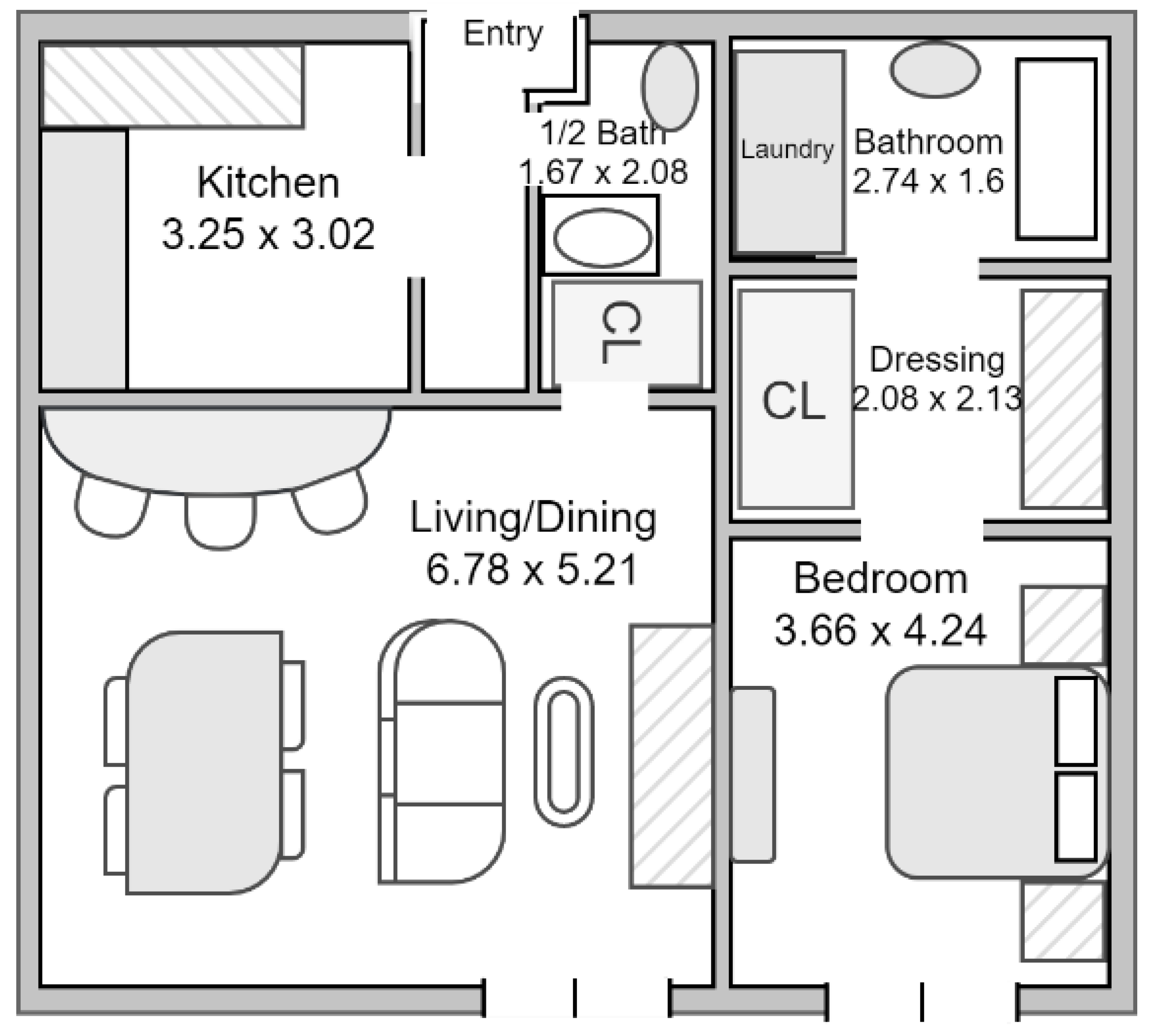
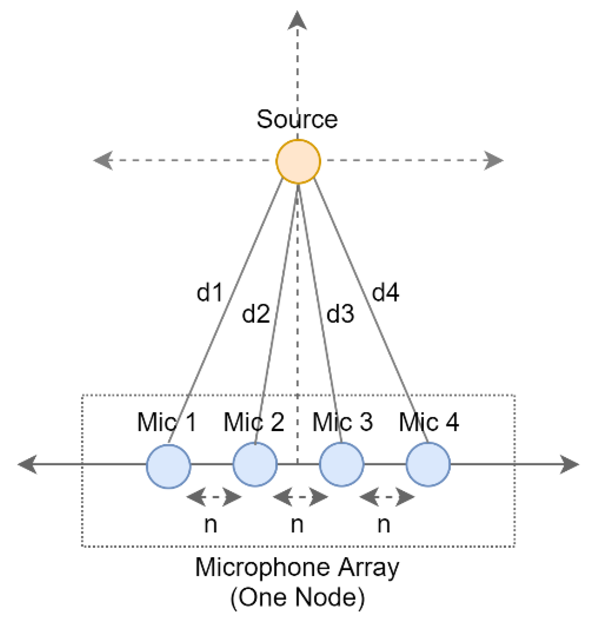
For this work, the generation of the synthetic database was done based on a 92.81 m² one-bedroom apartment modelled after the Hebrew Senior Life Facility [47], illustrated in Figure 2. We assumed a 3 m height for the ceiling. Multi-channel recordings were aimed for; hence, microphone arrays were placed on each of the four corners of the six rooms at 0.2 m below the ceiling. This produced four recordings, one from each of the receiver nodes.

Accordingly, the microphone arrays were composed of four linearly arranged omnidirectional microphones with 5 cm inter-microphone spacing (n), as per the geometry provided in Figure 3, where d refers to the distance from the sound source to the microphones.

Dry samples are taken from Freesound (FSD50K) [48], Kaggle [49], DESED Synthetic Soundscapes [50], and Open SLR [51], depending on the audio class. Due to the variations in sampling frequency, some of the audio signals were down sampled to 16 kHz for uniformity purposes. The room dimensions, source and receiver locations, wall reflectance, and other relevant information, were then used in order to calculate the impulse response for each room using the image method, incorporating source directivity [52]. This was then convolved with the sounds, specifying their location, in order to create the synthetic data. The data generated included clean signals, as well as different types of noisy signals, including: children playing, air conditioner, and street music, added at three different SNR levels: 15 dB, 20 dB, and 25 dB. The duration of each audio signal was uniformly kept at 5-s, as this was found to provide satisfactory time resolution for the sound scenes and events detected in this work.

Table 2. Summary of the Source Node Estimation Dataset.

Category	Training Data	Testing Data
Absence/Silence	11,286	876
Alarm	2765	260
Cat	11,724	1080
Dog	6673	792
Kitchen Activities	12,291	1062
Scream	4308	376
Shatter	2877	370
Shaver/toothbrush	11,231	1077
Slam	1565	268
Speech	30,113	2374
Water	6796	829
TOTAL	101,629	9364

describes this dataset. This data was curated such that the testing data consisted of one noise level for each node. Any instances of the data contained in the test set were then removed from the training data. The testing set content is summarized for a specific sound being recorded at four nodes:

• Node 1: Clean Signal with 15 dB Noise
• Node 2: Clean Signal with 20 dB Noise
• Node 3: Clean Signal with 25 dB Noise
• Node 4: Clean Signal

This ensures that even when the same sound is being recorded by the four nodes present, it reduces the chances of biasing through the addition of different types of noise at different SNR levels. Further, this was also designed to reflect real life recordings, where the sound from different microphones may differ based on their distance to the source and other sounds present in their surroundings.

As observed, audio classes used in the generation of this database focus on sound events and scenes that often occur, or require an urgent response, in dementia patients’ environment. Further, this was also generated through the room impulse responses of the HebrewLife Senior Facility [47], in order to reflect a realistic patient environment. This is because assistance monitoring systems are real-world applications of deep-learning audio classifiers, such as the work presented in this paper. Nonetheless, this can also be extended to other application domains as previously discussed.

3.2. Feature Extraction Using Fast CWT Scalograms

The CWT has several similarities to the Fourier transforms, such that it utilizes inner products in order to compute the similarity between the signal and an analysing function [53]. However, in the case of CWT, the analysing function is a wavelet, and the coefficients are the results of the comparison of the signal against shifted, scaled, and dilated versions of the wavelet, which are called constituent wavelets [53]. Compared with the STFT, wavelets provide better time-localization [30] and are more beneficial to non-stationary signals [53].

However, in order to reduce the computational requirements for deriving scalograms, this work proposes the use of the Fast Fourier Transform (FFT) algorithm for CWT coefficients computation [30]. Such that, if we define the mother wavelet (Ψ) to be [30], where t refers to continuous time:

$${\psi }_{ts}\left(u\right)=\frac{1}{\sqrt{t}}\psi \left(\frac{u-s}{t}\right)$$

(5)

Then Equation (3), involving the CWT coefficients, can be rewritten as follows [30], where $y_{avg}$ refers to the average of the four-channels of the audio signal:

$$CW{T}_c\left(s,t\right)={{\displaystyle \int }}_{-\infty }^{\infty }{y}_{avg}\left(u\right){\psi }_t^{*}\left(s-u\right)du$$

(6)

This shows that CWT coefficients can be expressed by the convolution of wavelets and signals. Thus, this can be written in the Fourier transform form domain, resulting in Equation (7) [30]:

$$CW{T}_c\left(s,t\right)=\frac{1}{2\pi }{{\displaystyle \int }}_{-\infty }^{\infty }{y}_{avg}\left(\omega \right){\psi }_{s,t}^{*}\left(\omega \right)d\omega$$

(7)

where ${\psi }_{s,t}^{*}\left(\omega \right)$ specifies the Fourier transform of the mother wavelet at scale t:

$${\psi }_{s,t}^{*}\left(\omega \right)=\sqrt{t}{\psi }^{*}\left(t\omega \right)e^{j\omega s}$$

(8)

Further, $y_{avg}\left(\omega \right)$ then denotes the Fourier transform of the analysed signal $y_{avg}\left(t\right)$:

$$y_{avg}\left(\omega \right)={{\displaystyle \int }}_{-\infty }^{\infty }{y}_{avg}\left(t\right)e^{j\omega t}dt$$

(9)

Hence, the discrete versions of the convolutions can be represented as per Equation (10), where n is in discrete time domain:

$$W\left(s\right)={{\displaystyle \sum }}_{n=0}^{N-1}{y}_{avg}\left(n\right){\psi }^{*}\left(s-n\right)$$

(10)

From the sum in Equation (10), we can observe that CWT coefficients can be derived from the repetitive computation of the convolution of the signal, along with the wavelets, at every value of the scale per location [30]. This work follows this process in order to extract the DFT of the CWT coefficients at a faster rate compared to the traditional method.

In summary, CWT coefficients are calculated through obtaining both the DFT of the signal, as per Equation (9), and the Morlet analysing function, as per Equation (8), via the FFT. The products of these are then derived and integrated, as per Equation (6), in order to extract the wavelet coefficients. Accordingly, the discrete version of the integration can be represented as a summation, which is observed in Equation (10).

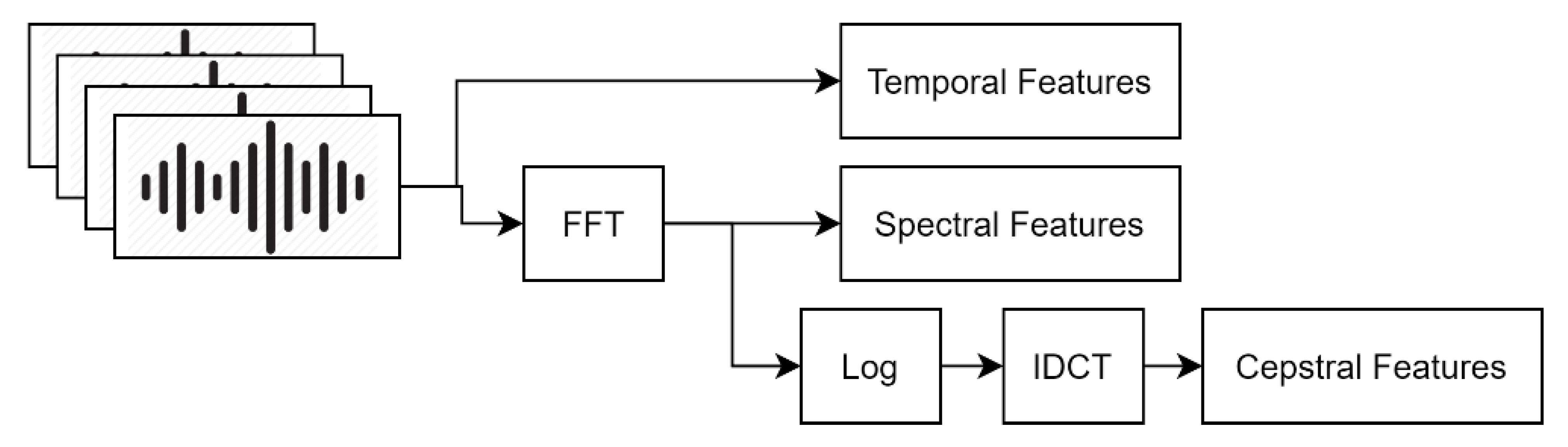
3.2.1. Feature Representation

Feature computation is carried out in MATLAB, exploiting functionalities provided in the Audio System and Data Communications toolboxes. A total of 20 filter bank channels with 12 cepstral coefficients are used for the cepstral feature extraction, as per the standard after DCT application [54]. An FFT size of 1024 is utilized, while the lower and upper filter bank frequency limits are set to 300 Hz and 3700 Hz. This frequency range includes the main components of speech signals (specifically, narrowband speech), while filtering out the humming sounds from the alternating current power, as well as high frequency noise [55]. Further, this range is relevant to the sound classes of speech and scream, and was found to also include the main components of the other classes. While larger frequency ranges could also be considered, this would require much larger FFT sizes to maintain the same frequency resolution, which in turn would increase the computational requirements. The extraction of the feature vectors is carried out by computing the average of the four time-aligned channels in the time domain, $y_{avg}\left(t\right)$. The coefficients are then extracted accordingly, from which single feature matrices are generated. The feature images are resized into 227 × 227 matrices using a bi-cubic interpolation algorithm with antialiasing [56], in order to match the input dimensionality of the AlexNet neural network model. 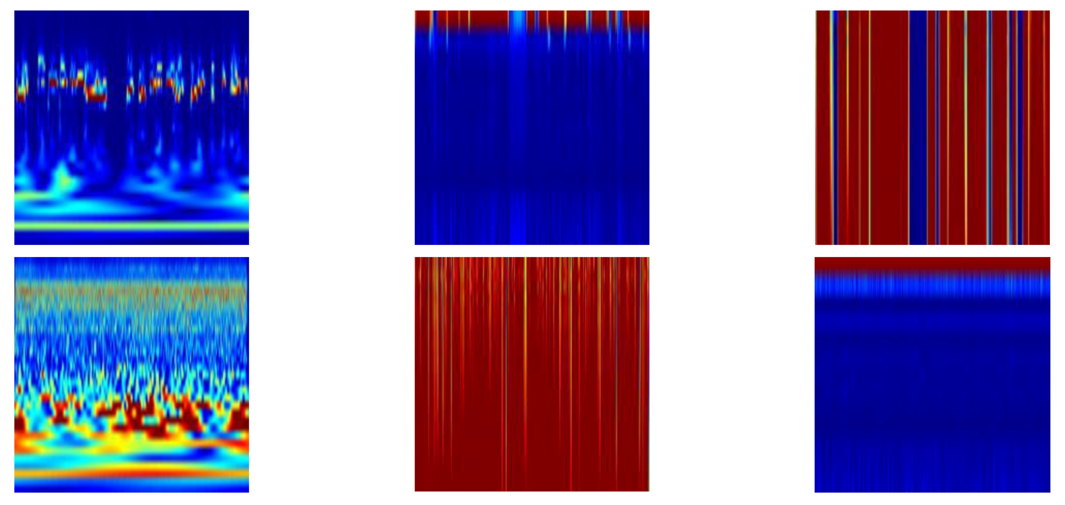Figure 4 shows samples of feature images for each of the three features compared, using the ‘Speech’ and ‘Kitchen sound’ classes.

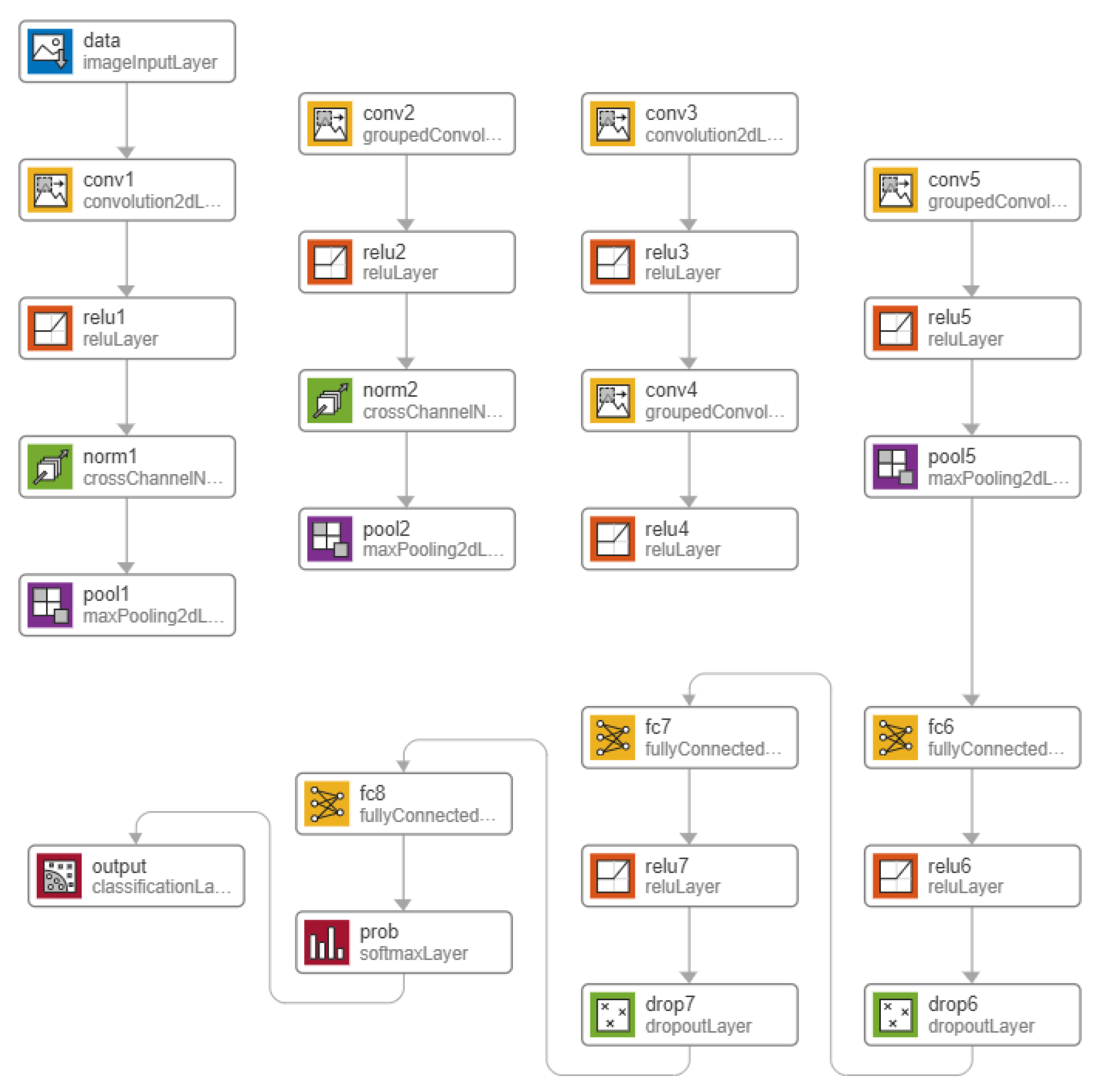
3.3. Modified AlexNet Network Model

Domestic multi-channel acoustic scenes consist of several signals that are captured with microphone arrays of different sizes and geometrical configurations. As discussed previously, CNNs have been widely popular for their advantage with regards to efficiency when used with data of spatial behaviour [57]. Thus, the experimentation part of this work compares different pre-trained network models for transfer learning. Modifications on the hyper-parameters are then made on the best performing network, the response being observed in three ways:

• Effects of changing the network activation function.
• Effects of fine-tuning the weight and bias factors, and parameter variation.
• Effects of modifications in the network architecture.

Activation functions in neural networks are a very important aspect of deep learning. These functions heavily influence the performance and computational complexity of the deep learning model [58]. Further, such functions also affect the network in terms of its convergence speed and ability to perform the task. Aside from exploring different activation functions, we also look at fine-tuning the weights and bias factors of the convolutional layers, as well as investigating the effects of the presence of convolutional layers based on performance.

For the modified AlexNet model, we examine the traditional Rectified Linear Unit (ReLU) activation function, along with three of its variations. The ReLU offers advantages in solving the vanishing gradient problem [59], which is common with the traditional sigmoid and tanh activation functions. The gradients of neural networks are computed through backpropagation, which calculates the derivatives of the network through every layer. Hence, for activation functions such as the sigmoid, the multiplication of several small derivatives causes a very small gradient value. This, in turn, negatively affects the update of weights and biases across training sessions [59]. Provided that the ReLU function has a fixed gradient of either 1 or 0, aside from providing a solution to the vanishing gradient problem and overfitting, it also results in lower computational complexity, and therefore significantly faster training. Another benefit of ReLUs is the sparse representation, which is caused by the 0 gradient for negative values [60]. Over time, it has been proven that sparse representations are more beneficial compared to dense representations [61].

Nonetheless, despite the numerous advantages of the ReLU activation function, there are still a number of disadvantages. Because the ReLU function only considers positive components, the resulting gradient has a possibility to go towards 0. This is because the weights do not get adjusted during descent for the activations within that area. This means that the neurons that will go into that state would stop responding to any variations in the input or the error, causing several neurons to die, which makes a substantial part of the network passive. This phenomena is called the dying ReLU problem [62]. Another disadvantage of the ReLU activation function is that values may range from zero to infinity. This implies that the activation may continuously increase to a very large value, which is not an ideal condition for the network [63]. The following activations attempt to mitigate the disadvantages faced by the traditional ReLU function through modifications and will be explored in this work:

• Leaky ReLU: The leaky ReLU is a variation of the traditional ReLU function that attempts to fix the dying ReLU problem by adding an alpha parameter, which creates a small negative slope when x is less than zero [64].
• Clipped ReLU: The clipped ReLU activation function attempts to prevent the activation from continuously increasing to a large value. This is achieved cutting the gradient at a pre-defined ceiling value [63].
• eLU: The exponential linear unit (eLU) is a similar activation function to ReLU. However, instead of sharply decreasing to zero for negative inputs, eLU smoothly decreases until the output is equivalent to the specified alpha value [65].

Aside from activation functions, variations in the convolutional and fully connected layers will also be examined. The study will be done in terms of both the number of parameters and the number of existing layers within the network.

For parameter modification, we explore the reduction of output variables in the fully connected layers. This method immensely reduces the overall network size [66]. However, it is important to note that recent works solely reduce the number of parameters from the first two fully connected layers. Hence, here we introduce the concept of uniform scaling, which is achieved by dividing the output parameters of fully connected layers by a common integer, based on the subsequent values.

Modification of the network architecture is also considered through examining the model’s performance when the number of layers within the network is varied. These layers may include convolutional, fully-connected, and activation function layers. Nonetheless, throughout the layer variation process, the model architecture is maintained to be of a series network type. A series network contains layers that are arranged subsequent to one another, containing a single input, and output layer. Directed Acyclic Graph (DAG) networks, on the other hand, have a complex architecture, from which layers may have inputs from several layers, and the outputs of which may be used for multiple layers [67]. The higher number of hidden neurons and weights, which is apparent on DAG networks, could increase risks of overfitting. Hence, maintaining a series architecture allows for a more customizable and robust network. Further, as per the state-of-the-art, all other compact networks that currently exist present a DAG architecture. Thus, the development of a compact network with a more customizable format, and through using fewer layers, proposes advantages in designing sturdy custom networks.

3.4. Performance Evaluation Metrics

To evaluate the performance of the proposed systems, the following aspects are investigated:

• Per class and overall comparison of different cepstral, temporal, and spectro-temporal features classified using various pre-trained neural network and machine learning models.
• Effects of balancing the dataset

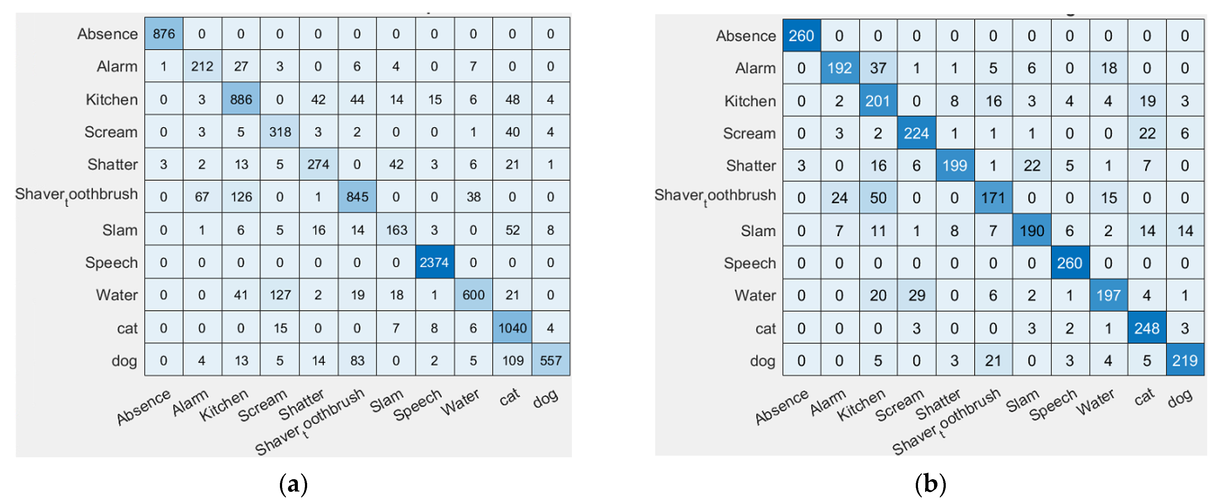
Aside from the standard accuracy, evaluations of the performances of different techniques were also compared and measured in terms of their F1-scores. This is defined to be a measure that takes into consideration both the recall and the precision, which are derived from the ratios of True Positives (TP), True Negatives (TN), False Positives (FP), and False Negatives (FN) [68], which can be extracted from confusion matrices.

The databases used for this research compose of unequal numbers of audio files per category. To account for the data imbalance, two different techniques are used:

• Balancing the Dataset

Particularly used for the initial development and experiments conducted for this work, in this technique, the dataset was equalized across all levels in order to preserve a balanced dataset. This is done in order to avoid biasing in favour of specific categories with more samples. It is achieved by reducing the amount of data per level to match the minimum amount of data amongst the categories. Selection of the data was done randomly throughout the experiments.

2.

Using Weight-sensitive Performance Metrics

Provided that the F1-score serves as the main performance metric used for the experiments conducted, it is crucial to ensure that these metrics are robust and unbiased, especially for multi-classification purposes. When taking the average F1-score for an unbalanced dataset, the amount of data per level may affect and skew the results for the mean F1-score in favour of the classes with the most amount of data. Therefore, we consider three different ways of calculating the mean F1-score, including the Weighted, Micro, and Macro F1-scores, in order to take into account for the dataset imbalance [69].

4. Results

4.1. Feature Extraction Results

Comparison of Cepstral, Spectral, and Spectro-Temporal Features

Per-level and average comparisons using MFCC and Log-Mel spectrogram features against the proposed CWTFT scalograms method are seen in

Table 3. Per-level comparison between imbalanced and balanced data between different types of features, with an average of three training trials.

CWTFT Scalograms
	Imbalanced Data				Balanced Data
Category	Accuracy	Precision	Recall	F1-Score	Accuracy	Precision	Recall	F1-Score
Silence	100.0%	99.3%	100.0%	99.7%	100.0%	98.4%	100.0%	99.2%
Alarm	65.4%	63.4%	65.4%	64.4%	75.2%	83.8%	75.2%	78.7%
Cat	97.2%	82.3%	97.2%	89.1%	94.8%	77.9%	94.8%	86.1%
Dog	74.8%	74.3%	74.8%	74.5%	84.7%	89.2%	84.7%	85.8%
Kitchen	82.3%	82.4%	82.3%	82.4%	76.5%	59.3%	76.5%	67.2%
Scream	83.7%	82.4%	83.7%	83.1%	85.9%	85.2%	85.9%	86.1%
Shatter	78.2%	72.2%	78.2%	75.1%	75.4%	89.8%	75.4%	83.2%
Shaver	71.5%	83.0%	71.5%	76.8%	66.7%	75.2%	66.7%	69.5%
Slam	65.4%	70.6%	65.4%	67.9%	71.5%	82.1%	71.5%	77.6%
Speech	100.0%	97.8%	100.0%	98.9%	100.0%	92.1%	100.0%	96.7%
Water	74.2%	85.8%	74.2%	79.6%	75.2%	82.2%	75.2%	78.1%
Micro	86.0%	86.0%	86.0%	86.0%	82.4%	83.2%	82.4%	82.6%
Weight	86.0%	86.0%	86.0%	85.9%	82.4%	83.2%	82.4%	82.6%
Macro	81.2%	81.2%	81.2%	81.0%	82.4%	83.2%	82.4%	82.6%
MFCCs
	Imbalanced Data				Balanced Data
Category	Accuracy	Precision	Recall	F1-Score	Accuracy	Precision	Recall	F1-Score
Absence	100.0%	98.6%	100.0%	99.3%	100.0%	98.7%	100.0%	99.3%
Alarm	53.2%	69.7%	53.2%	60.4%	52.3%	79.4%	52.3%	62.3%
Cat	75.6%	62.6%	75.6%	68.5%	74.1%	65.3%	74.1%	72.0%
Dog	74.8%	69.7%	74.8%	72.1%	76.9%	79.4%	76.9%	78.1%
Kitchen	64.1%	71.6%	64.1%	67.7%	51.8%	48.3%	51.8%	49.2%
Scream	75.8%	71.9%	75.8%	73.8%	76.4%	74.1%	76.4%	74.3%
Shatter	69.1%	53.8%	69.1%	60.5%	72.5%	70.2%	72.5%	73.1%
Shaver	53.8%	69.6%	53.8%	60.7%	48.6%	43.8%	48.6%	45.6%
Slam	37.9%	53.0%	37.9%	44.2%	50.1%	70.6%	50.1%	57.8%
Speech	99.1%	97.0%	99.1%	98.0%	99.1%	86.3%	99.1%	94.0%
Water	48.7%	55.5%	48.7%	51.9%	50.2%	50.9%	50.2%	50.1%
Micro	77.6%	77.6%	77.6%	77.6%	68.4%	69.7%	68.4%	68.7%
Weight	77.6%	77.3%	77.6%	77.3%	68.4%	69.7%	68.4%	68.7%
Macro	68.4%	70.3%	68.4%	68.8%	68.4%	69.7%	68.4%	68.7%
Log-Mel Spectrograms
	Imbalanced Data				Balanced Data
Category	Accuracy	Precision	Recall	F1-Score	Accuracy	Precision	Recall	F1-Score
Absence	100.0%	98.4%	100.0%	99.2%	100.0%	100.0%	100.0%	100.0%
Alarm	62.5%	61.2%	62.5%	61.8%	70.2%	62.2%	70.2%	65.6%
Cat	73.4%	65.0%	73.4%	68.9%	55.9%	60.3%	55.9%	61.2%
Dog	52.2%	51.4%	52.2%	51.8%	49.8%	54.9%	49.8%	51.9%
Kitchen	51.8%	42.6%	51.8%	46.7%	32.3%	31.6%	32.3%	32.6%
Scream	43.9%	47.4%	43.9%	45.6%	54.4%	53.6%	54.4%	54.3%
Shatter	58.2%	62.2%	58.2%	60.1%	66.8%	64.2%	66.8%	65.8%
Shaver	43.1%	41.2%	43.1%	42.1%	41.9%	31.4%	41.9%	38.1%
Slam	20.2%	36.3%	20.2%	26.0%	37.2%	56.1%	37.2%	44.4%
Speech	99.1%	92.8%	99.1%	95.9%	98.1%	82.9%	98.1%	89.5%
Water	32.2%	38.7%	32.2%	35.1%	35.2%	40.7%	35.2%	37.1%
Micro	65.0%	65.0%	65.0%	65.0%	58.3%	58.0%	58.3%	58.2%
Weight	65.0%	63.9%	65.0%	64.2%	58.3%	58.0%	58.3%	58.2%
Macro	57.9%	57.9%	57.9%	57.6%	58.3%	58.0%	58.3%	58.2%

, which is an average of three training trials. As observed, F1-score averaging is done using three different methods: Micro, Macro, and Weighted, in order to take into account the biasing that may be caused by the data imbalance. Further, the table also entails the comparison of the system performance between imbalanced and balanced data. To achieve a balanced data, the size of the dataset is reduced to match the lowest numbered category in both training and testing sets. As per Table 2, for each category, this turns out to be 1565 files for training, based on the “Slam” category, and 260 files for testing, based on the “Alarm” category. This adds up to a total of 17,215 training files and 2860 testing files.

The following results are achieved using the traditional AlexNet network, provided that this gives us the highest results as per our previous works [45,46]. Training for the imbalanced data is achieved at 10 epochs with 1016 iterations per epoch. However, it is important to note that the number of epochs for the balanced data is 75, as it has less iterations per epoch due to the lower amount of data per category. Hence, it requires more epochs in order to reach stability.

As observed, the CWTFT scalograms have consistently achieved the highest F1-score across all categories, exceeding the performance of the MFCC features by over 10%. As mentioned earlier, this can be explained by the spectro-temporal properties of wavelets, which allows excellent time and frequency localization. The Log-Mel spectrograms gather the least F1-score out of the three features. In terms of the data imbalance, it is observed that once data is even across all categories, it improves the performance of the smaller categories. Nonetheless, the trade-off is that it reduces the F1-score for the categories with more data initially. It is also evident that performances associated with classes referring to acoustic scenes are higher than those associated to sound events. This is because sound events occur sporadically and at different instances throughout the 5-s intervals, whereas sound scenes are continuously present throughout the duration. Overall, the imbalanced dataset returns higher performance. Figure 5 accordingly shows the relevant confusion matrices for imbalanced and balanced datasets.

In our previous works, we examined the response of the system performance by concatenating the cepstra from individual channels [45,46]. This yielded a slightly better performance than using a single cepstrum after averaging the four time-aligned channels for the case of cepstral coefficients. Extracting cepstral coefficients for each channel allows a thorough consideration of all distinctive properties of the signal, which minimizes the loss of information. However, per-channel feature extraction did not cause improvement with Scalogram features, yielding a result of 90.72% as opposed to 92.33% for averaging the channels, as audio sources are already separated within its wavelet computation process.

Aside from the accuracy, execution time for the inference and resource requirements is another important consideration that must be made when selecting features.

Table 4. Average execution time for inference (in s).

Parameter	Scalograms	MFCC	Log-Mel
Feature Extraction Execution Time	0.1981	1.0076	1.0640

details the execution time information for the three features compared, in terms of extracting the relevant features and translating them into a 227 × 227 image. Recording the execution time was achieved through a machine with Intel Core i7-9850H CPU @ 2.60 GHz processor, operated in single core. The reported execution times are in seconds and are an average of 100 different readings. As observed, scalograms also returned the shortest overall time duration across all three features compared. The numerous processes involved with the MFCC and Log-mel features justify the longer extraction time.

CWTFT coefficients are derived through taking the product between the DFT of the signal and the analyzing function through FFT, and inverting this in order to extract the wavelet coefficients. On the other hand, both MFCC and Log-Mel are based on the Mel-scale filter bank. This is based on the short-term analysis, from where vectors are computed per frame. Further, windowing is performed to remove discontinuities, prior to utilizing the DFT to generate the Mel filter bank. Further processes, such as the use of triangular filters and warping, are also necessary prior to the application of the IDFT and transformation.

It is important to note that in terms of memory usage, there are negligible differences between the three features compared. This is because the features are being resized and translated into a 227 × 227 image through bi-cubic interpolation, in order to fit the classifier. Nonetheless, each image translation occupies between 4–12 KB of memory, depending on the sound class.

4.2. Architecture of Modified AlexNet-33 (MAlexNet-33)

This section discusses the results achieved through the detailed study of the effects of modifying the traditional AlexNet architecture. The AlexNet model was found to result in the highest F1-scores based on our previous work experiments [45,46]. In this work, we aim to improve this network by decreasing the overall network size while maintaining its performance. To begin with, the original layer structure of the AlexNet network is presented in Figure 6. As observed, it contains 25 layers, with 2 regular convolution layers, 3 group convolution layers, and 3 fully connected layers.

4.2.1. Exploring Variations of the Rectified Linear Unit and the Number of Layers

For this experiment, the response of the system to reducing the number of layers is investigated. Further, different variations of the ReLU activation function are also examined.

Table 5. Performance Measures of Different Networks using Variations of the F1-score.

Network	Type	Accuracy	Precision	Recall	F1-Score
AlexNet	Micro	86.36%	86.36%	86.36%	86.36%
	Weighted	86.36%	86.72%	86.36%	86.24%
	Macro	81.03%	82.99%	81.03%	81.69%
AlexNet-20	Micro	85.19%	85.19%	85.19%	85.19%
	Weighted	85.19%	86.01%	85.19%	85.02%
	Macro	79.68%	82.42%	79.68%	80.44%
AlexNet-20 with eLU (1)	Micro	84.30%	84.30%	84.30%	84.30%
	Weighted	84.30%	84.80%	84.30%	84.18%
	Macro	78.08%	81.20%	78.08%	79.22%
AlexNet-20 with Leaky ReLU (0.01)	Micro	85.70%	85.70%	85.70%	85.70%
	Weighted	85.70%	86.37%	85.70%	85.58%
	Macro	79.45%	83.62%	79.45%	80.99%
AlexNet-20 with Clipped ReLU (6)	Micro	84.10%	84.10%	84.10%	84.10%
	Weighted	84.10%	84.25%	84.10%	84.04%
	Macro	78.38%	78.55%	78.38%	78.26%
AlexNet-17 with Leaky ReLU (0.01)	Micro	81.89%	81.89%	81.89%	81.89%
	Weighted	81.89%	82.67%	81.89%	81.74%
	Macro	75.04%	76.39%	75.04%	75.13%

displays the different combinations tested for this experiment with regards to decreasing the number of layers and changing the activation function, presented as an average between 11 classes. Hence, throughout the results, it is apparent that the micro averaging results between the four measures are the same and there are close similarities between some of the measures. This is due to the total number of false negatives and false positives being the same. More distinct differences between the classes can be seen in the per-level comparison, such as that of Table 3.

From Table 5, AlexNet-20 was achieved by removing one grouped convolutional, two ReLU, one fully connected, and one 50% dropout layer from the original network. It is observed that removing convolutional and fully connected layers from the network reduces its performance as well.

However, it is also apparent that using other activation functions improves the performance. For instance, using a Leaky ReLU with a 0.01 parameter in place of the ReLU activation function increased the weighted F1-score to 85.58%, having less than 1% difference from the original network’s performance. Such improvement is reportedly due to the Leaky ReLU’s added parameter to solve the dying ReLU problem. Due to having less layers in the system, a reduction of about 30% from the original size was also achieved. MAlexNet-20 with a Leaky ReLU activation function has a network size of about 150 MB, compared against AlexNet’s 220 MB network size.

Subsequent to this, the concept of a successive activation function was also looked at. For this, two activation function layers were placed successively throughout the network. However, as per

Table 6. Successive Activation Function Combination Summary.

Activation Function 1	Activation Function 2	Accuracy	Network Size
ReLU	ReLU	83.27%	157.92 MB
Leaky ReLU (0.01)	Leaky ReLU (0.01)	84.32%	157.92 MB
ReLU	Leaky ReLU (0.01)	85.38%	157.92 MB
Tanh	Leaky ReLU (0.01)	73.49%	157.92 MB

, it is implied that using two successive activation functions does not necessarily improve the overall system performance. However, it is also apparent that using more than one activation function does not affect the overall size of the network.

4.2.2. Parameter Modification

The AlexNet contains three fully connected layers with parameter values of 9216, 4096, and 4096 for the inputs, and 4096, 4096, and 1000 for the outputs. In this experiment, we reduce the output parameters across the first two fully connected layers within the network through scaling. The results achieved from this experiment are reported in

Table 7. Parameter Modification Results.

Activation Function	Input to FC6	FC6	FC7	Num. of Layers	Scale	Epochs	Network Size	Weighted F1
ReLU	9216	4096	4096	25 (orig *)	None	10	221.4 MB	86.24%
ReLU	4608	574	574	25 (equ *)	Equ.	30	31.90 MB	85.76%
ReLU	4608	576	256	25 (div 16)	16	30	31.23 MB	85.15%
Leaky ReLU (0.01)	4608	576	256	25 (div 16)	16	30	31.23 MB	85.48%
Leaky ReLU (0.01)	4608	384	172	25 (div 24)	24	30	23.82 MB	86.82%
ReLU	4608	384	192	25 [64]	None	30	23.85 MB	85.76%

* orig—refers to the original AlexNet layer; equ—refers to using equal fully connected layer parameters.

.

In here, FC6 refers to the output of the first fully connected layer, and FC7 refers to the output of the second fully connected layer. It is important to note that the output of the last fully connected layer corresponds to the number of classes the system aims to identify and is not determined by parameter scaling.

As observed from Table 7, a notable improvement is observed through scaling the output parameters of the fully connected layers through a division of 24 (from the input parameter and fully connected sizes of the original network), which provided slightly higher F1-score compared to the original AlexNet. Further, this results in an almost 90% reduction in size of the network compared to the original (23.82 MB as opposed to 221.4 MB). Uniform scaling also returns better performance compared to keeping an equal number of parameters across all fully connected layers. Further, it also achieved a higher weighted F1-score than the combination used by previous recent studies, for which the exact parameters used are represented by the last entry on Table 7 [66]. It is important to note that the input size for FC6 is automatically calculated for the modified networks. After the convolution stages, this is found to be 4608 parameters. Quantitatively, it is implied that the output parameters of all fully connected layers subsequent to the last fully connected layer can be scaled down extensively, depending on the number of classes that the model is designed to predict, keeping in mind that the fully connected output parameters are higher than the number of possible predictions.

The number of epochs required is determined through the training accuracy and losses graph. Generally, a lower number of output parameters slows down the training, requiring more epochs in order to reach a well-learned network. Figure 7 displays the difference between a traditional AlexNet and a version with lower numbers of output parameters in the fully connected layers. The comparison was done for 10 epochs.

4.2.3. The Combination of Layer and Parameter Modification

Provided that uniformly scaling the fully connected layer parameters has proven beneficial, in this section, we combine this technique with the advantages of modifying the number of layers. This is done in two ways, the results for which are presented in

Table 8. Results for the combination of layer and parameter modifications.

Activation Function	FC6	FC7	Num. of Layers	Scale	Epochs	Network Size	Weighted F1
ReLU	384	192	23 (n.conv4)	None	30	21.19 MB	84.63%
Leaky ReLU (0.01)	384	192	23 (n.conv4)	None	30	21.19 MB	83.05%
Leaky ReLU (0.01)	576	-	20 (n.conv4)	None	30	27.98 MB	83.80%
Leaky ReLU (0.01)	1064	-	20 (n.conv4)	Equ.	30	45.99 MB	84.66%
ReLU	1064	-	20 (n.conv4)	Equ.	30	45.99 MB	82.54%
ReLU	576	-	20 (n.conv4)	Equ.	30	27.99 MB	83.63%
Leaky ReLU (0.01)	576	-	20 (n.conv4)	Equ.	30	27.99 MB	83.71%
Leaky ReLU (0.01)	576	-	22 (w.conv4)	Equ.	30	30.64 MB	85.00%
Leaky ReLU (0.01)	384	-	22 (w.conv4)	24	30	23.56 MB	85.76%
Leaky ReLU (0.01)	384	172	23 (n.conv4)	24	30	21.16 MB	84.76%
Leaky ReLU (0.01)	384	172	27 (gconv64)	24	30	17.34 MB	86.89%
Leaky ReLU (0.01)	192	86	27 (gconv64)	48	30	13.59 MB	85.61%
Leaky ReLU (0.01)	384	172	33 (gconv32)	24	30	14.33 MB	87.92%

:

• Decreasing the number of layers: Similar to the experiment conducted in Section 3.2.1, this reduces the number of convolutional and fully connected layers within the network. For example, MAlexNet-23 refers to the removal of conv4 and relu4, maintaining all fully connected layers. On the other hand, MAlexNet-20 is the same network structure examined in Section 3.2.1.
• Increasing the number of layers: For this experiment, another grouped convolutional layer/s with the relevant activation function was added to the network structure. From the original AlexNet model, the grouped convolutions carry bias learnable weights of 1 × 1 × 192 × 2 and 1 × 1 × 128 × 2, respectively. For this work, additional grouped convolution functions were added, such that it has a bias learnable weight of 1 × 1 × 64 × 2 for MAlexNet-27, and 1 × 1 × 64 × 2 and 1 × 1 × 32 × 2 for MAlexNet-33. Accordingly, Leaky ReLu (0.01) activation functions were utilized for all grouped convolutional layers.

As per Table 8, it is observed that the top performing algorithm is the MAlexNet-33, which is designed as a combination of both fully connected parameter scaling, as well as the addition of two new grouped convolutional layers with bias learnable weights of 1 × 1 × 64 × 2 and 1 × 1 × 32 × 2, and relevant activation layers. This provided a weighted F1-score of 87.96%, exceeding the performance of the AlexNet, with a network size of 14.33 MB. This suggests an over 95% decrease in the size of the resource requirements when compared to the original model. When compared to [66], this also improved both the performance and the network size, exceeding the performance by around 2.16% and decreasing the network size by over 40%. Aside from the improvement in resource requirements, decreasing the network size also returned a notable improvement in the inference execution time, provided that they are factors linearly related to one another.

4.2.4. Comparison with Other Compact Networks

In this section, a comparison of the proposed architecture to currently existing compact networks is presented. For this work, several compact pre-trained models including SqueezeNet [42], MobileNet-v2 [70], NasNet Mobile [71], and ShuffleNet [72], are considered. A summary of the comparison is seen in

Table 9. Detailed Comparison with other Compact Neural Networks.

	MAlexNet-33	SqueezeNet	MobileNet-v2	NasNet Mobile	ShuffleNet
Number of Layers	33	68	155	913	173
Depth	8	18	53	N/A	50
Type	Series Network	DAG	DAG	DAG	DAG
Network Size	14.33 MB	3.07 MB	9.52 MB	19.44 MB	3.97 MB
Activation Function	Leaky ReLU (0.01)	Fire ReLU	Clipped ReLU (C: 6)	ReLU	ReLU
Weighted F1-score	87.92%	84.48%	86.85%	83.38%	86.91%
Training time	178 min	273 min	599 min	1668 min	792 min
Epochs	30	30	30	30	30
Loading time average	1.10 s	1.04 s	1.32 s	2.59 s	1.62 s
Execution time average	0.0148 s	0.0159 s	0.0338 s	0.1345 s	0.0348 s

, in terms of the total number of layers, depth, type, network size in MB, the activation function used, the weighted F1-score, the training time for 30 epochs, the network loading time, and the execution inference time average. The network loading time is an average of five trials, while the execution time is measured in 100 trials.

Throughout the comparison, it is important to note that, while MAlexNet-33 is a series network, all other compact networks are DAG networks, which have a complex architecture and a significantly larger number of layers.

As observed, our proposed network consistently provided the highest weighted F1-score in comparison to the other compact networks. Despite having a 14.33 MB network size, this provided negligible time differences (about 0.08-s against SqueezeNet) in terms of loading the network. Further, it also possesses the least training and execution time compared to the other networks.

It is also apparent that other compact networks possess a higher loading time despite the smaller network size, which is caused by the DAG network configuration, and the multiple layers within the architecture. Provided that the MAlexNet-33 has the least number of layers, it creates a highly customizable network architecture. Adding more layers of neurons increases the complexity of the neural networks. Although hidden layers are crucial for extracting the relevant features, having too many hidden layers may cause overfitting. In this case, the network would be limited in terms of its generalization abilities. In order to avoid this effect, this work focuses on designing a smaller network with fewer neurons and weights than a traditional compact neural network.

5. Discussion

Interpreting the presented results, we conclude that the use of CWTFT scalograms returns the best results for audio scene and event classification applications. This is supported by our previous experiments, which were performed using the SINS database [45,46] and the experiments conducted in this work. This can be justified by the fact that scalograms possess excellent time and frequency localization. Furthermore, another advantage is that it also separates audio sources upon the wavelet computation process. Using an FFT-based wavelet transform also returns favourable time duration requirements, which exceeded that of cepstral and spectral features.

There are three main discoveries found in this study:

Hypothesis 1:

The Leaky ReLU activation function returned higher performance for multi-level classification as opposed to the traditional ReLU in the majority of cases.

Verification of Hypothesis 1: This is true on a case-by-case scenario. This can be explained by the presence of the dying ReLU problem in feature sets, which is ameliorated through the small parameter added through the Leaky ReLU. However, it is important to note that the presence of the dying ReLU problem could depend on several factors, including the nature of the data being trained. In cases where this does not occur, replacing the activation function to a Leaky ReLU may not return any advantages.

Hypothesis 2:

Decreasing the number of fully connected and convolutional layers throughout the network also slightly decreases the performance.

Verification of Hypothesis 2: Generally, convolutional layers represent high level features within the network. Accordingly, fully connected layers flatten and combine these features. Hence, reducing the number of these layers negatively affects the performance of the network.

Hypothesis 3:

Decreasing parameters, weight factors, and biases within the fully connected and convolutional layers helps decrease the size of the network more, compared to when these layers are removed completely.

Verification of Hypothesis 3: Both convolutional and fully connected layers contribute to the high and low-level features from which the network learns, and are therefore essential. However, since pre-trained models are originally trained on very large data, large parameters, weight, and bias factors are often not necessary for the smaller dataset by which transfer learning is being implemented for. This explains the maintenance of the system performance despite decreasing the parameters for these layers accordingly. Based on our experiments, scaling the parameters uniformly across fully connected layers returns the best performance.

6. Conclusions

This study started with a per-level performance comparison against top-performing feature extraction methodologies, which demonstrated the robustness of the proposed CWTFT features. Further, an extensive study on pre-trained neural network modification was also presented, aiming to reduce the size of the AlexNet model whilst maintaining the accuracy. The top performing methodology involved the use of FFT-based CWT Scalogram features, with a modified AlexNet model with 33 layers (MAlexNet-33). This model uses the Leaky ReLU as its main activation function, combining strategies of both including additional convolutional layers and uniformly scaling the parameters of convolutional and fully connected layers in order to create the optimum network. The best performance resulted in an 87.92% weighted F1-score at a network size of 14.33 MB. This suggests a good improvement when compared with using the original AlexNet network with the same features, which resulted in an F1-score of 86.24%, at a size of 221.4 MB.

References

1. Almaadeed, N.; Asim, M.; Al-ma’adeed, S.; Bouridane, A.; Beghdadi, A. Automatic Detection and Classification of Audio Events for Road Surveillance Applications. Sensors 2018, 18, 1858. [Google Scholar] [CrossRef] [Green Version]
2. Lozano, H.; Hernaez, I.; Picon, A.; Camarena, J.; Navas, E. Audio Classification Techniques in Home Environments for Elderly/Dependant People. In Proceedings of the ICCHP 2010, Vienna, Austria, 14–16 July 2010; pp. 320–323. [Google Scholar]
3. Lecouteux, B.; Vacher, M.; Portet, F. Distant Speech Recognition in a Smart Home: Comparison of Several Multisource ASRs in Realistic Conditions. In Proceedings of the INTERSPEECH 2011, Florence, Italy, 27–31 August 2011. [Google Scholar]
4. Mitilineos, S.A.; Potirakis, S.M.; Tatlas, N.A.; Rangoussi, M. A Two-level Sound Classification Platform for Environmental Monitoring. Hindawi J. Sens. 2018, 2018, 2–13. [Google Scholar] [CrossRef]
5. Imoto, K. Introduction to acoustic event and scene analysis. Acoust. Sci. Technol. 2018, 39, 182–188. [Google Scholar] [CrossRef] [Green Version]
6. Adavanne, S.; Parascandolo, G.; Pertila, P.; Heittola, T.; Virtanen, T. Sound Event Detection in Multichannel Audio Using Spatial and Harmonic Features. In Proceedings of the DCASE 2016, Budapest, Hungary, 3 September 2016. [Google Scholar]
7. Dekkers, G.; Vuegen, L.; van Waterschoot, T.; Vanrumste, B.; Karsmakers, P. DCASE 2018—Task 5: Monitoring of domestic activities based on multi-channel acoustics. arXiv 2018, arXiv:1807.11246. [Google Scholar]
8. Serizel, R.; Bisot, V.; Essid, S.; Richard, G. Acoustic Features for Environmental Sound Analysis. In Computational Analysis of Sound Scenes and Events; Springer: Cham, Switzerland, 2017; pp. 71–101. [Google Scholar]
9. Valenti, M.; Squartini, S.; Diment, A.; Parascandolo, G.; Virtanen, T. A Convolutional Neural Network Approach for Acoustic Scene Classification. In Proceedings of the DCASE2016 Challenge, Budapest, Hungary, 8 February–7 September 2016. [Google Scholar]
10. Chen, H.; Zhang, P.; Bai, H.; Yuan, Q.; Bao, X.; Yan, Y. Deep Convolutional Neural Network with Scalogram for Audio Scene Modeling. In Proceedings of the INTERSPEECH 2018, Hyderabad, India, 2–6 September 2018. [Google Scholar]
11. Lee, M.; Lee, Y.K.; Lim, M.T.; Kang, T.K. Emotion Recognition using Convolutional Neural Network with Selected Statistical Photolethysmogram Features. Appl. Sci. 2020, 10, 3501. [Google Scholar] [CrossRef]
12. Srinivasu, P.N.; SivaSai, J.G.; Ijaz, M.F.; Bhoi, A.K.; Kim, W.; Kang, J.J. Classification of Skin Disease Using Deep Learning Neural Networks with MobileNet V2 and LSTM. Sensors 2021, 21, 2852. [Google Scholar] [CrossRef] [PubMed]
13. Ristea, N.C.; Radoi, A. Complex Neural Networks for Estimating Epicentral Distance, Depth, and Magnitude of Seismic Waves. IEEE Geosci. Remote. Sens. Lett. 2021, 1–5. [Google Scholar] [CrossRef]
14. Peeters, G. A large set of audio features for sound description (similarity and classification) in the CUIDADO project. In Proceedings of the IRCAM, Paris, France, 23–24 June 2004. [Google Scholar]
15. Sahidullah, M.; Saha, G. Design, analysis and experimental evaluation of block based transformation in MFCC computation for speaker recognition. Speech Commun. 2012, 54, 543–565. [Google Scholar] [CrossRef]
16. Zheng, F.; Zhang, G.; Song, Z. Comparison of different implementations of MFCC. J. Comput. Sci. Technol. 2001, 16, 582–589. [Google Scholar] [CrossRef]
17. Ravindran, S.; Demirogulu, C.; Anderson, D. Speech Recognition using filter-bank features. In Proceedings of the 37th Asi-lomar Conference on Signals, Systems, and Computers, Pacific Grove, CA, USA, 9–12 November 2003. [Google Scholar]
18. Le Roux, J.; Vincent, E.; Mizuno, Y.; Kameoka, H.; Ono, N.; Sagayama, S. Consistent Wiener Filtering: Generalized Time-Frequency Masking Respecting Spectrogram Consistency. In Latent Variable Analysis and Signal Separation. LVA/ICA 2010. Lecture Notes in Computer Science; Vigneron, V., Zarzoso, V., Moreau, E., Gribonval, R., Vincent, E., Eds.; Springer: Berlin/Heidelberg, Germany, 2010; Volume 6365. [Google Scholar]
19. Choi, W.; Kim, M.; Chung, J.; Lee, D.; Jung, S. Investigating Deep Neural Transformations for Spectrogram-based Musical Source Separation. In Proceedings of the International Society for Music Information Retrieval, Montreal, QC, Canada, 11–16 October 2020. [Google Scholar]
20. Gerkmann, T.; Krawezyk-Becker, M.; Roux, J. Phase processing for single-channel speech enhancement: History and recent advances. IEEE Signal Process. Mag. 2015, 32, 55–66. [Google Scholar] [CrossRef]
21. Zheng, W.; Mo, Z.; Xing, X.; Zhao, G. CNNs-based Acoustic Scene Classification using Multi-Spectrogram Fusion and Label Expansions. arXiv 2018, arXiv:1809.01543. [Google Scholar]
22. Chu, S.; Kuo, C.; Narayanan, S.; Mataric, M. Where am I? Scene Recognition for Mobile Robots using Audio Features. In Proceedings of the 2006 IEEE International Conference on Multimedia and EXPO, Toronto, ON, USA, 9–12 July 2006. [Google Scholar]
23. Inou, T.; Vinayavekhin, P.; Wang, S.; Wood, D.; Greco, N.; Tachibana, R. Domestic Activities Classification based on CNN using Shuffling and Mixing Data Augmentation. In Proceedings of the DCASE2018, Surrey, UK, 19–20 November 2018. [Google Scholar]
24. Tanabe, R.; Endo, T.; Nikaido, Y.; Ichige, T.; Nguyen, P.; Kawaguchi, Y.; Hamada, K. Multichannel Acoustic Scene Classification by Blind Dereverberation, Blind Source Separation, Data Augmentation, and Model Ensembling. In Proceedings of the DCASE2018, Surrey, UK, 19–20 November 2018. [Google Scholar]
25. Mesaros, A.; Heittola, T.; Virtanen, T. Acoustic Scene Classification: An Overview of DCASE 2017 Challenge Entries. In Proceedings of the 2018 16th International Workshop on Acoustic Signal Enhancement (IWAENC), Tokyo, Japan, 17–20 September 2018. [Google Scholar]
26. Schroder, J.; Goetze, S.; Anemuller, J. Spectro-Temporal Gabor Filterbank Features for Acoustic Event Detection. IEEE/ACM Trans. Audio Speech Lang. Process. 2015, 23, 2198–2208. [Google Scholar] [CrossRef]
27. Cotton, C.V.; Ellis, D.P.W. Spectral vs. spectro-temporal features for acoustic event detection. In Proceedings of the 2011 IEEE Workshop on Applications of Signal Processing to Audio and Acoustics (WASPAA), New Paltz, NY, USA, 20–23 October 2011; pp. 69–72. [Google Scholar]
28. Wolf, G.; Mallat, S.; Shamma, S. Audio source separation with time-frequency velocities. In Proceedings of the 2014 IEEE International Workshop on Machine Learning for Signal Processing (MLSP), Reims, France, 21–24 September 2014; pp. 1–6. [Google Scholar]
29. Sejdic, E.; Djurovic, I.; Stankovic, L. Quantitative Performance Analysis of Scalogram as Instantaneous Frequency Estimator. IEEE Trans. Signal Process. 2008, 56, 3837–3845. [Google Scholar] [CrossRef]
30. Komorowski, D.; Pietraszek, S. The Use of Continuous Wavelet Transform Based on the Fast Fourier Transform in the Analysis of Multi-channel Electrogastrography Recordings. J. Med Syst. 2016, 40, 1–15. [Google Scholar] [CrossRef] [PubMed] [Green Version]
31. Zhou, Y.; Hu, W.; Liu, X.; Zhou, Q.; Yu, H.; Pu, Q. Coherency feature extraction based on DFT-based continuous wave-let transform. In Proceedings of the IEEE PES Asia-Pacific Power and Energy Engineering Conference (APPEEC), Brisbane, Australia, 15–18 November 2015. [Google Scholar]
32. Phan, H.; Hertel, L.; Maass, M.; Koch, P.; Mazur, R.; Mertins, A. Improved Audio Scene Classification Based on Label-Tree Embeddings and Convolutional Neural Networks. IEEE/ACM Trans. Audio Speech Lang. Process. 2017, 25, 1278–1290. [Google Scholar] [CrossRef] [Green Version]
33. Dang, A.; Vu, T.; Wang, J. Acoustic Scene Classification using Convolutional Neural Network and Multi-scale Multi-Feature Extraction. In Proceedings of the IEEE International Conference on Consumer Electronics, Las Vegas, NV, USA, 12–14 January 2018. [Google Scholar]
34. Krishna, S.; Kalluri, H. Deep Learning and Transfer Learning Approaches for Image Classification. Int. J. Recent Technol. Eng. 2019, 7 (Suppl. 4), S427–S432. [Google Scholar]
35. Curry, B. An Introduction to Transfer Learning in Machine Learning; Medium: San Francisco, CA, USA, 2018. [Google Scholar]
36. Zabir, M.; Fazira, N.; Ibrahim, Z.; Sabri, N. Evaluation of Pre-Trained Convolutional Neural Network Models for Object Recognition. Int. J. Eng. Technol. 2018, 7, 95. [Google Scholar] [CrossRef]
37. Krizhevsky, A.; Sutskever, I.; Hinton, G.E. Imagenet classification with deep convolutional neural networks. Commun. ACM 2012, 60, 1097–1105. [Google Scholar] [CrossRef]
38. Szegedy, C.; Liu, W.; Jia, Y.; Sermanet, P.; Reed, S.; Anguelov, D.; Erhan, D.; Vanhoucke, V.; Rabinovich, A. Going Deeper with Convolutions. In Proceedings of the 2015 IEEE Conference on Computer Vision and Pattern Recognition (CVPR), Boston, MA, USA, 7–12 June 2015; pp. 1–9. [Google Scholar]
39. He, K.; Zhang, X.; Ren, S.; Sun, J. Deep residual learning for image recognition. In Proceedings of the IEEE Conference on Computer Vision and Pattern Recognition, Las Vegas, NV, USA, 27–30 June 2016. [Google Scholar]
40. Szegedy, C.; Ioffe, S.; Vanhoucke, V.; Alemi, A. Inception-v4, Inception-ResNet and the Impact of Residual Connections on Learning. In Proceedings of the Thirty-First AAAI Conference on Artificial Intelligence (AAAI-17), San Francisco, CA, USA, 4–9 February 2017. [Google Scholar]
41. Chollet, F. Xception: Deep Learning with Depthwise Separable Convolutions. In Proceedings of the IEEE Conference on Computer Vision and Pattern Recognition (CVPR), Honolulu, HI, USA, 21–26 July 2017. [Google Scholar]
42. Iandola, F.; Han, S.; Moskewicz, M.; Ashraf, K.; Dally, W.; Keutzer, K. SqueezeNet: AlexNet-Level Accuracy with 50× Fewer Parameters and <0.5MB model size. In Proceedings of the ICLR 2017, Toulon, France, 24–26 April 2017. [Google Scholar]
43. Simonyan, K.; Zisserman, A. Very deep convolutional networks for large-scale image recognition. arXiv 2014, arXiv:1409.1556. [Google Scholar]
44. LeCun, Y.; Bottou, L.; Bengio, Y.; Haffner, P. Gradient-based learning applied to document recognition. Proc. IEEE 1998, 86, 2278–2324. [Google Scholar] [CrossRef] [Green Version]
45. Copiaco, A.; Ritz, C.; Fasciani, S.; Abdulaziz, N. Scalogram Neural Network Activations with Machine Learning for Domestic Multi-channel Audio Classification. In Proceedings of the 2019 IEEE International Symposium on Signal Processing and Information Technology (ISSPIT), Ajman, United Arab Emirates, 10–12 December 2019; pp. 1–6. [Google Scholar]
46. Copiaco, A.; Ritz, C.; Abdulaziz, N.; Fasciani, S. Identifying Optimal Features for Multi-channel Acoustic Scene Classification. In Proceedings of the ICSPIS Conference, Dubai, United Arab Emirates, 18–19 December 2019; pp. 1–4. [Google Scholar]
47. Hebrew SeniorLife. Available online: https://www.hebrewseniorlife.org/newbridge/types-residences/independent-living/independent-living-apartments (accessed on 27 January 2021).
48. Fonseca, E.; Plakal, M.; Font, F.; Ellis, D.P.; Serra, X. Audio Tagging with Noisy Labels and Minimal Supervision. In Proceedings of the Detection and Classification of Acoustic Scenes and Events 2019 Workshop (DCASE2019), New York, NY, USA, 25–26 October 2019. [Google Scholar]
49. Takahashi, N.; Gygli, M.; Pfister, B.; Van Gool, L. Deep Convolutional Neural Networks and Data Augmentation for Acoustic Event Recognition. In Proceedings of the INTERSPEECH 2016, San Francisco, CA, USA, 8–12 September 2016. [Google Scholar]
50. Turpault, N.; Serizel, R.; Salamon, J.; Shah, A.P. Sound Event Detection in Domestic Environments with Weakly Labeled Data and Soundscape Synthesis. In Proceedings of the Detection and Classification of Acoustic Scenes and Events 2019 Workshop (DCASE2019), New York, NY, USA, 25–26 October 2019. [Google Scholar]
51. He, F.; Chu, S.H.; Kjartansson, O.; Rivera, C.; Katanova, A.; Gutkin, A.; Demirsahin, I.; Johny, C.; Jansche, M.; Sain, S.; et al. Open-source Multi-speaker Speech Corpora for Building Gujarati, Kannada, Malayalam, Marathi, Tamil and Telugu Speech Synthesis Systems. In Proceedings of the 12th LREC Conference, Marseille, France, 11–16 May 2020. [Google Scholar]
52. Hafezi, S.; Moore, A.H.; Naylor, P.A. Room Impulse Response for Directional source generator (RIRDgen). 2015. Available online: http://www.commsp.ee.ic.ac.uk/~ssh12/RIRD.htm (accessed on 31 March 2021).
53. MATLAB Documentation, Continuous Wavelet Transform and Scale-Based Analysis. 2019. Available online: https://www.mathworks.com/help/wavelet/gs/continuous-wavelet-transform-and-scale-based-analysis.html (accessed on 31 March 2021).
54. Tiwari, R.; Agrawal, K.K. Normalized Cepstral Coefficients based Isolated Word Recognition for Oral-tradition Tribal Languages using Scaled Conjugate Gradient Method. J. Crit. Rev. 2020, 7, 2097–2107. [Google Scholar]
55. Dinkar Apte, S. Random Signal Processing; CRC Press: Boca Raton, FL, USA, 2018. [Google Scholar]
56. Han, D. Comparison of Commonly Used Image Interpolation Methods. In Proceedings of the 2nd International Conference on Computer Science and Electronics Engineering (ICCSEE 2013), Hangzhou, China, 22–23 March 2013. [Google Scholar]
57. Hirvonin, T. Classification of Spatial Audio Location and Content Using Convolutional Neural Networks. In Proceedings of the Audio Engineering Society 138th Convention, Warsaw, Poland, 7–10 May 2015. [Google Scholar]
58. Wang, Y.; Li, Y.; Song, Y.; Rong, X. The Influence of the Activation Function in a Convolution Neural Network Model of Facial Expression Recognition. Appl. Sci. 2020, 10, 1897. [Google Scholar] [CrossRef] [Green Version]
59. Weir, M. A method for self-determination of adaptive learning rates in back propagation. Neural Netw. 1991, 4, 371–379. [Google Scholar] [CrossRef]
60. Shi, S.; Chu, X. Speeding up Convolutional Neural Networks by Exploiting the Sparsity of Rectifier Units. arXiv 2017, arXiv:1704.07724. [Google Scholar]
61. Hu, W.; Wang, M.; Liu, B.; Ji, F.; Ma, J.; Zhao, D. Transformation of Dense and Sparse Text Representations. In Proceedings of the 28th International Conference on Computational Linguistics, Barcelona, Spain, 8–13 December 2020; pp. 3257–3267. [Google Scholar]
62. Lu, L.; Shin, Y.; Su, Y.; Karniadakis, G. Dying ReLU and Initialization: Theory and Numerical Examples. Commun. Comput. Phys. 2020, 28, 1671–1706. [Google Scholar] [CrossRef]
63. Doshi, C. Why Relu? Tips for Using Relu. Comparison between Relu, Leaky Relu, and Relu-6; Medium: San Francisco, CA, USA, 2019. [Google Scholar]
64. Maas, A.; Hanuun, A.; Ng, A. Rectifier nonlinearities improve neural network acoustic models. In Proceedings of the ICML, Atlanta, GA, USA, 16–21 June 2013. [Google Scholar]
65. Djork-Arne, C.; Unterthiner, T.; Hochreiter, S. Fast and accurate deep network learning by exponential linear units (ELUs). In Proceedings of the ICLR, San Juan, Puerto Rico, 2–4 May 2016. [Google Scholar]
66. Romanuke, V. An Efficient Technique for Size Reduction of Convolutional Neural Networks after Transfer Learning for Scene Recognition Tasks. Appl. Comput. Syst. 2018, 23, 141–149. [Google Scholar] [CrossRef] [Green Version]
67. Mathworks. DAG Network, Matlab Documentation. 2017. Available online: https://www.mathworks.com/help/deeplearning/ref/dagnetwork.html (accessed on 31 March 2021).
68. Phung, S.L.; Bouzerdoum, A.; Nguyen, G.H. Learning pattern classification tasks with imbalanced data sets. In Pattern Recognition; Yin, P., Ed.; In-Tech: Vukovar, Croatia, 2009; pp. 193–208. [Google Scholar]
69. Shmueli, B. Multi-Class Metrics Made Simple, Part II: The F1-Score, towards Data Science. 2019. Available online: https://towardsdatascience.com/multi-class-metrics-made-simple-part-ii-the-f1-score-ebe8b2c2ca1 (accessed on 31 March 2021).
70. Sandler, M.; Howard, A.; Zhu, M.; Zhmoginov, A.; Chen, L. Mobilenetv2: Inverted Residuals and Linear Bottlenecks. In Proceedings of the 2018 IEEE Conference on Computer Vision and Pattern Recognition (CVPR), Salt Lake City, UT, USA, 18–23 June 2018. [Google Scholar]
71. Zoph, B.; Vasudevan, V.; Shlens, J.; Le, Q.V. Learning Transferable Architectures for Scalable Image Recognition. In Proceedings of the 2018 IEEE/CVF Conference on Computer Vision and Pattern Recognition, Salt Lake City, UT, USA, 18–23 June 2018; pp. 8697–8710. [Google Scholar]
72. Zhang, X.; Zhou, X.; Lin, M.; Sun, J. ShuffleNet: An Extremely Efficient Convolutional Neural Network for Mobile Devices. In Proceedings of the 2018 IEEE/CVF Conference on Computer Vision and Pattern Recognition, Salt Lake City, UT, USA, 18–23 June 2018. [Google Scholar]
Figure 1. Taxonomy of features extracted from audio.
Applsci 11 04880 g001
Figure 2. Floorplan of one-bedroom apartment used as acoustic environment for the synthetic database, dimensions in meters [47].
Applsci 11 04880 g002
Figure 3. Microphone array geometry for a single node: four linearly spaced microphones.
Applsci 11 04880 g003
Figure 4. Feature representation samples using the ‘Speech’ (top) and ‘Kitchen’ (bottom) classes: Left to Right: CWT Scalograms, Log-Mel, and MFCC.
Applsci 11 04880 g004
Figure 5. Confusion matrices for the top performing algorithm—CWTFT scalograms for: (a) Imbalanced dataset using the full synthetic database; (b) balanced dataset with 1565 files for training, and 260 files for testing.
Applsci 11 04880 g005
Figure 6. AlexNet Network Layer Structure: This is a 25-layer series architecture imported via Matlab Deep Network Designer. The CNN model accepts 227 × 227 image inputs and is trained to classify between 1000 image classes via ImageNet.
Applsci 11 04880 g006
Figure 7. Training accuracy and losses graph (Left) AlexNet; (Right) Modified AlexNet with less parameters.
Applsci 11 04880 g007