A Linearized Approach for the Electric Light Commercial Vehicle Routing Problem Combined with Charging Station Siting and Power Distribution Network Assessment

Abstract

Transportation electrification has demonstrated a significant position on power utilities and logistic companies, in terms of assets operation and management. Under this context, this paper presents the problem of seeking feasible and good quality routes for electric light commercial vehicles considering battery capacity and charging station siting on the power distribution system. Different transportation patterns for goods delivery are included, such as the capacitated vehicle routing problem and the shortest path problem for the last mile delivery. To solve the problem framed within a mixed integer linear mathematical model, the GAMS software is used and validated on a test instance conformed by a 19-customer transportation network, spatially combined with the IEEE 34 nodes power distribution system. The sensitivity analysis, performed during the computational experiments, show the behavior of the variables involved in the logistics operation, i.e., routing cost for each transport pattern. The trade-off between the battery capacity, the cost of the charging station installation, and energy losses on the power distribution system is also shown, including the energy consumption cost created by the charging operation.

1. Introduction

Pollution on the environment represents a worldwide topic for discussion, due to the impact on the air quality and general population. During the last two decades, there has been an increase of 66% approximately on global CO${}_2$ emissions, according to International Energy Agency data. In terms of oil energy demand, the participation of the transport sector declined in advanced economies (most developed countries in the world) throughout 2019. Nevertheless, this reduction is overtaken by the increase in transport sector oil energy demand from the rest of the countries [1]. In this context, transportation electrification becomes a prominent measure to tackle global warming produced by greenhouse gas emissions. Electric mobility is getting larger at a markable pace, China being the most extensive EV market in the world, followed by Europe and the United States. Economic instruments and incentives for zero and low emissions vehicles, translated into public policies, are often created to shorten the cost gap between conventional and Electric Vehicles EVs, and improve the charging infrastructure development. Investment in this latter is being boosted by different power sector stakeholders, charging hardware manufacturers, utilities, and charging point operators. Current policies forecast that global EV stock will reach about 135 million vehicles in 2030. A more ambitious scenario, named EV30@30, estimates 250 million of global EV stock, considering an expeditious implementation of policies that promote a 30% market share for EVs in all modes by 2030 [2].

Large logistics companies involved in goods delivery, i.e., Fedex, Amazon, UPS, and DHL, are committed to introducing electric trucks in their fleets, looking to decrease the carbon emissions in the supply chain. Particularly, electric Light Commercial Vehicles eLCVs are being used for bringing products to customers in the framework of eco-friendly goods distribution. From this perspective, although there has been progress in range extension and battery manufacturing, the driving range still represents a technical issue towards a higher deployment of these vehicles in terms of scheduling and routing [3]. According to manufacturers, the typical mileage of eLCVs is in the range of 100 to 170 km; nonetheless, this feature is directly affected by acceleration, speed, breaking, and other factors related with driving behavior. Payload weight and uncontrollable exogenous factors, such as topography and outdoor temperature, are also involved in battery range performance [4]. Due to the limited range of eLCVs to successfully complete delivery routes as part of the intra-city operations, it is necessary to develop optimal routing schemes that comprise detours to charging stations as an effort to overcome the “range anxiety” [5]. In the context of eLCVs, routing plans can be properly designed considering the Electric Vehicle Routing Problem EVRP, which is the extended version of the classical Capacitated Vehicle Routing Problem CVRP. A fixed number of EVs leave from a depot to meet the merchandise demand for a set of customers. Once the customers are visited, the EVs return to the depot to complete the route. Due to the electric nature, these vehicles are required to visit charging stations in the intra-route operations when the battery is depleted. Charging facilities are limited and dispersed across the transportation network [6].

As shown throughout the works mentioned in Section 2, the EVRP has been largely studied with different perspectives; nonetheless, the power distribution system is not introduced as part of the mathematical model that covers the operation of logistics company and the power utility, which properly fits into real-world scenarios. The charging process requires a huge quantity of energy that can affect the power network in terms of energy losses, voltage drop, and introduction of harmonics and components lifetime [7], it being necessary to look for suitable and proper siting of charging stations considering both transportation and power distribution networks. In this sense, this paper presents a novel mathematical model for the approach named the electric Light Commercial Vehicles Routing Problem with Charging Station Location and impact on Power Distribution System eLCVRP-CS-PDS. The proposal is an extension of the work performed in [8,9], and the mathematical formulation is solved using the GAMS/CPLEX solver. The contributions are identified as follows:

• An improved mixed integer linear programming model is proposed in a three-index formulation, considering the traditional CVRP approach, last mile delivery problem LMDP framed within the shortest path context, siting of charging stations, and power distribution system assessment.
• Prior research on EVRP and location for EV charging stations are assumed fixed. In this work, siting of charging stations and EVRP are considered in a whole within the same mathematical formulation. Hence, it is possible to decide whether a charging station is installed at a certain candidate point, depending on routing needs, battery range, energy consumption in the charging operation, and energy losses on the power distribution network.
• Candidate points for charging stations can be sited either on each customer or at a different spatial location, making this approach be within a more realistic framework.
• The proposed model considers multiple visits to a charging station, regardless of the transport pattern followed by the EV.
• A sensitivity analysis to support decision-making is performed to demonstrate the charging station needs along the transportation network, contingent upon the battery technology in terms of energy capacity.

The remainder of this paper is organized as follows: Section 2 presents a revision of the literature review around the EVRP and the gaps in terms of considering the power distribution system. The mathematical model of the eLCVRP-CS-PDS, including the formulation of transport patterns, charging station location, and linear power flow approach, is shown in Section 3. In Section 4, the test system is presented, combining the power distribution system and the transportation network. Likewise, different computational experiments are performed using a sensitivity analysis as a function of battery capacity variation. Section 5 presents the conclusions of this work and avenues of research, including some final reflections.

2. Literature Review

To the best of our knowledge, early contributions on the EVRP have been examined as an extension of the problem called the GVRP Green Vehicle Routing Problem introduced by [10]. This approach is a variation of the well-known Vehicle Routing Problem VRP, considering that a set of alternative fuel vehicles with limited autonomy needs to recharge at alternative fuel stations along the execution of their duties. Restrictions account for the maximum duration of the route, and a fixed service time is considered for refueling operation and customer visit. GVRP can be considered as the baseline for the EVRP. Several works have been published in the same research pipeline. In [11], the EVRP is described as a modified and comprehensive version of the VRP using Electric Vehicles, being an NP-Hard problem that requires substantial computational effort even for medium scale instances. In this sense, the authors in [12] are one step further in the GVRP, presenting a methodology to introduce refueling stations along the GVRP routes, with outstanding outcomes related with the updating part of the best-known solutions in the standard benchmark cases of the problem. Furthermore, in [13], the routing problem with EVs is studied taking into consideration more realistic elements, such as partial recharges and the different charging technologies.

For the sake of the convenience, the literature review is presented in chronological order, considering works published in different academic and scientific databases. The EVRP is a relatively new problem in the specialized literature with a starting point presented in the GVRP, firstly introduced by [10] in 2012, as a generic of green logistics problem. Thereafter, an improved approach with electric and fuel-engined vehicles is found in [14], encompassing the original and reduced graph where the battery power consumption is included along the edges. Later, in 2015, time windows’ constraints and the use of charging stations are incorporated in the EVRP by the authors of [15], allowing partial battery recharge and seeking to reduce charging time along the route. In the next year (2016), a similar contribution is presented in [16], formulating the problem as a mixed integer linear programming model, defining a decision variable that reflects the battery state of charge. The problem is solved using the Adaptive Large Neighborhood Search Algorithm ALNS. Beyond the traditional contributions, the decision-making analysis proposed by the authors in [17] reveals the influence of different factors in the charging station location for EVs, such as service availability, engineering feasibility, and economic, social, environmental, and land factors.

Subsequently, in 2017, various works for EVRP are found in relation with time windows and heterogeneous fleet [18,19]. The power distribution system is incorporated, considering grid ancillary services with Vehicle to Grid, whilst warranting optimal routing. Nonlinear charging is also introduced in the same period, providing a closer approach to the charging process that could affect the EV routing time [20]. Furthermore, routing efficiency is an additional feature mentioned in [21] for the transportation electrification. The research deals with a data-driven method for EV energy consumption prediction based on external disturbances. Similar to the work presented in [17], in [22], a decision-making framework suitable for investors is performed, providing the optimal location of charging facilities in residential areas.

Through the papers analyzed for 2018, in [23], the time operation is minimized on a fleet of electric vans, taking into account that energy required to go through an arc of the transportation network may be influenced not only by the distance, but also by the current cargo load. Similar contributions can be identified from the stochastic perspective in [24], defining random features for the energy cost of each road segment, due to environmental factors. From different perspectives, the review performed in [25] shows the trends of optimal placement of charging stations for EVs at the level of power distribution system, transportation network, and logistics, including the demand and supply chain; and the barriers provided by the existing infrastructure for a large-scale deployment of EVs. The review discusses the modeling approaches used by the researchers in this area, considering the objective functions, constraints, and proposed optimization algorithms. Likewise, how the charging infrastructure has developed in different countries, which is strongly related to economic, social, and technological conditions. In regard with the recharging needs, the authors of [26] propose a mixed integer linear programming model where two approaches are treated: limited range and limited emissions for the electric and conventional vehicles, respectively. The problem is formulated based on a fixed location for recharge/refuel stations, with an existing trade-off between the objectives: energy cost, routing time, cost of emissions, and battery degradation. An extension of the work in [16] is presented by the same authors in [27] that shows two mathematical formulations for the EVRP allowing fast charging using multiple types of charging equipment. The problem is solved using exact techniques and ALNS for small and large-size instances, respectively. Some research is focused on battery swapping as an alternative to overcome the barriers of the charging stations in terms of charging duration that results in delays on the routing operation. That is the case of the work presented in [28], where it is proposed an EVRP model in conjunction with material handling problem for automotive assembly lines. A mathematical model is proposed in [9] considering the transportation and power distribution networks, with the CVRP and the conventional power flow equations based on the voltage drop and the balance of active and reactive power at the nodes. Although the approach is partially at the level of the work contributions in the present manuscript, the mathematical model presents nonlinearities related with calculation of currents through the electrical branches, and the assumption that the power distribution system is balanced, i.e., one-phase representation.

Along the revised works belonging to the period 2019, the main contributions lie on extended proposals for EVRP. In [29], the Dynamic capacitated EVRP is treated as a complex version of the conventional EVRP, making the number of customers variable during the routing execution. Furthermore, the work presented in [30] provides an improved version of the EVRP introducing Hybrid EVs, with the advantage that, during routing operation, the vehicle is able to go to either a gas station to refuel or a charging station to recharge, depending on the mode selection. On the other hand, the work in [31] represents an attractive formulation for goods delivery, since the transportation network is composed by nodes tagged as customers, battery swapping stations, and satellite stations. A common depot is the departure point with available freight, which is transported to the transfer or satellite stations. Then, small EVs are used to deliver the freight to the customers. In terms of efficiency for EV routing operation, in [32], an estimation of the energy consumed throughout the routing is computed as an objective function to be minimized, based on detailed speed profile and topography of the segments between visited nodes. Likewise, in [33], the EVRP is formulated within the uncertainties around the energy consumption. These are related with load weight and physical characteristics of the vehicle that converges in a longitudinal dynamics model. For the charging process context, the work presented in [34], which is similar to [20], addresses the nonlinear charging considering a concave function. This is translated into a benefit from the mathematical model perspective, as it can deal with a linear approach to warrant an optimal solution. Related efforts are stated in [35] that focuses on linearizing the nonlinear function of the EV charging operation, considering piece-wise linear approximations, applied for partial recharge and different charging technologies. From other perspectives, the user satisfaction is also considered in the EV charging stations deployment, which is analyzed in [36] via three indicators: charging convenience, charging cost, and charging time. The same authors of [9] published in [8] a linear approach for the EVRP; furthermore, the three-index formulation for the CVRP is not used, particularly for the parcel flows through the arcs of routes. In this sense, the drawback comes with the charging stations’ installation limited to the customers location, which does not reflect the complete reality.

Contributions corresponding to 2020 are framed within topics on nonlinear partial recharge, time windows, multiple depots, bin packing problem, battery swapping, and battery efficiency. Likewise, some efforts are made around the analysis of influencing factors for EV market penetration. This is the case for the work reported in [37], which proposes the technological progress assessment of EVs for logistics purposes, considering physical and performance features. The work performed in [38] is towards the same direction, making a comparison between the conventional EV and other low-emission freight transportation means technologies, such as biodiesel, natural gas, and fuel-cells. In [39], the EVRP with time windows and multiple recharging options is investigated, with partial recharge and battery swapping. The formulation represents a cost-efficient routing strategy, since the driver can recharge the battery according to the energy requirement for traveling completion or choose battery swapping for purposes of saving routing time. In the charging process context, the authors in [40] introduce the EVRP with load-dependent battery discharge and nonlinearities in the charging process, fitted within a linearized mathematical model. In the same streamline, the proposal in [41] works with a fuzzy optimization model taking into consideration the uncertain behavior of some parameters, such as travel time, service time, and battery energy consumption. Like other contributions mentioned above, partial recharge is allowed with the purpose of making the model more practical from a realistic point of view. In order to avoid the installation of charging stations, in [42], the option to open multiple depots is shown to comply with the demand of customers using a fixed number of EVs that are fairly distributed on each corresponding depot. A more advanced approach is proposed in [43] where the EVRP with multiple depots is proposed, incorporating two-dimensional weighted items for each customer demand, as part of the bin packing problem that is also considered as an NP-hard problem. Given the computational complexity, the formulation is solved using variable neighborhood search and space saving algorithms for the EV routing and bin packing problems, respectively. Similar to the contributions in [30], in [44], the routing problem for PHEVs and power management optimization is integrated. First, PHEVs tours are computed, then the driving cycle profile of each tour is obtained as a function of the customers assigned to that tour. This information is the data input to find optimal power distribution from the two energy sources installed in a PHEV. In contrast with traditional approaches, a prominent focus to overcome the waiting times of recharge and the so called range anxiety is posed in [5], combining the EVRP with mobile battery swapping vans, both synchronized at a designated time and space. In the context of battery efficiency, the research in [45] implements a simulator for an electric truck to achieve the least-energy delivery route, taking into consideration the nonlinear model of the battery and the change of parcel weight over the course of the route.

As far as we know, all the aspects of our proposal are not covered by the works for EVRP previously presented. Most of them do not consider both the transportation and power distribution networks within a mathematical model, neither different shipping patterns, i.e., considering the capacitated vehicle routing problem and the last mile delivery problem. Thus, we present and solve the eLCVRP-CS-PDS as part of the relationship between the transportation network and power distribution system, via the charging station considered as the point of common coupling. A linear approach of the power flow is used to assess the electrical grid operation, supported by an affine constraint.

3. Methods

In this section, the formal description and the mathematical formulation of the eLCVRP-CS-PDS are presented. Given a network conformed by customers and electrical nodes scattered along the space, the eLCVRP-CS-PDS intends to obtain a set of routes traveled by a fixed number of homogeneous light commercial EVs that depart from and arrive to a common depot. As the EVs travel the corresponding route, customer demand is met, considering that, in the intermediate of the route, if necessary, the EV is required to visit a charging station located at an electrical node, before the battery is depleted. In agreement with the current technology, we assume a fast charging process that does not affect the duration of the route, and that the state of charge of the battery is reduced in a linear proportion with the distance traveled. Additionally, another group of EVs with a lower battery capacity is used to execute the last mile delivery approach. The vehicles depart from and arrive to known origin and destination points, traveling the shortest path between both points, and considering that a charging station must be visited if required. Throughout the mathematical formulation, there are a set of constraints able to control whether a charging station should be installed at an electrical node, depending on the battery capacity. In addition, the intended charging station can receive multiple visits from the same or different EVs.

The eLCVRP-CS-PDS proposed in this work can be described as a graph theory problem. Let $G=(V,A)$ be a complete graph with a set of vertices $V=N\cup C$ and a set of arcs A with the interconnection of all vertices. Set $N=\left\{1,\dots ,n\right\}$ represents the customer vertices where index 1 is the depot, and set $C=\left\{n+1,\dots ,n+c\right\}$ describes the charging station candidate points corresponding to the power distribution network. Each arc and customer are associated with distance $d_{ij}$ and merchandise demand $D_i$, respectively. Due to the homogeneous nature of the fleet, all of the vehicles are featured by a constant capacity for cargo and batteries. It is necessary to point out that there are two patterns identified for the EVs running into this problem: a group of EVs follow the CVRP approach, with a battery capacity larger than that for those EVs designated for the last mile delivery problem, which corresponds to the other group of EVs. Thus, the constraints of the mathematical model are split into several components: CVRP approach, last mile delivery problem, charging stations location, and a linear proposal of power flow in electrical distribution systems. For better understanding, we first describe the nomenclature, followed by the constraints of the model and the objective function.

3.1. CVRP: The Three-Index Formulation

Throughout the description of the mathematical model, we denote $Dep$ as the depot for the Capacitated Vehicle Routing Problem or CVRP approach. This latter implies that a fleet of vehicles with a corresponding cargo capacity depart from a depot, visit several customers to meet their goods demand, and return to the depot. The demand of the customers must be fully met, seeking routes at a minimum traveling cost [46]. The CVRP is represented by Equations (1)–(13), considering the relation with the candidate points of charging stations and a fixed number of EVs. Notice that “\” is the except symbol and refers to the “individual” that is not included in a set. For example: $\forall i\in NDep$, this means: For all i that belongs the set N, except the depot; in other words, the index i can take any value stored in N, except the value assigned for the depot $Dep$.

$$\begin{array}{c}\hfill \sum _{kϵK}{Y}_{i,k}=1,\forall iϵN\setminus \left\{Dep\right\}\end{array}$$

(1)

$$\begin{array}{c}\hfill \sum _{iϵN}\sum _{kϵK}{X}_{i,j,k}=1,\forall jϵN\setminus \left\{Dep\right\}\end{array}$$

(2)

$$\begin{array}{c}\hfill \sum _{jϵN}\sum _{kϵK}{X}_{i,j,k}=1,\forall iϵN\setminus \left\{Dep\right\}\end{array}$$

(3)

$$\begin{array}{c}\hfill \sum _{kϵK}\sum _{jϵN}{X}_{Dep,j,k}=\left|K\right|\end{array}$$

(4)

$$\begin{array}{c}\hfill \sum _{kϵK}\sum _{jϵN}{X}_{j,Dep,k}=\left|K\right|\end{array}$$

(5)

$$\sum _{\begin{array}{c}jϵV\\ i\ne j\end{array}}{X}_{i,j,k}-\sum _{\begin{array}{c}jϵV\\ i\ne j\end{array}}{X}_{j,i,k}=0\forall iϵV\forall kϵK$$

(6)

$$\begin{array}{c}\hfill \sum _{jϵN}{X}_{j,i,k}=Y_{i,k}\forall iϵN\forall kϵK\end{array}$$

(7)

$$\sum _{\begin{array}{c}jϵN\\ j\ne h\end{array}}{t}_{h,j,k}\le \left[\sum _{\begin{array}{c}iϵN\\ h\ne i\end{array}}{t}_{i,h,k}-D_h·x_{i,h,k}\right]+Cap·\left[1-\sum _{\begin{array}{c}iϵN\\ h\ne i\end{array}}{x}_{i,h,k}\right]\forall hϵN\setminus \left\{Dep\right\}\forall kϵK$$

(8)

$$\sum _{\begin{array}{c}iϵN\\ i\ne h\end{array}}{t}_{i,h,k}=\sum _{\begin{array}{c}jϵN\\ h\ne j\end{array}}{t}_{h,j,k}\forall hϵC\setminus \left\{Dep\right\}\forall kϵK$$

(9)

$$\begin{array}{c}\hfill t_{i,h,k}\ge 0\forall iϵV\forall hϵV\forall kϵKi\ne h\end{array}$$

(10)

$$\begin{array}{c}\hfill t_{i,h,k}\le Cap·x_{i,h,k}\forall iϵV\forall hϵV\forall kϵKi\ne h\end{array}$$

(11)

$$\sum _{\begin{array}{c}iϵV\end{array}}\sum _{\begin{array}{c}kϵK\end{array}}{x}_{i,h,k}=BigM·Y_h^{cvrp}\forall hϵC$$

(12)

$$\sum _{\begin{array}{c}iϵV\\ i\ne Dep\end{array}}\sum _{\begin{array}{c}kϵK\end{array}}{t}_{Dep,i,k}=\sum _{\begin{array}{c}iϵV\\ i\ne Dep\end{array}}{D}_i$$

(13)

Constraint (1) imposes that each customer is visited exactly once. Constraints (2) and (3) are indegree and outdegree constraints, which impose that exactly one arc enters and leaves each vertex associated with each customer, respectively. Likewise, constraints (4) and (5) show that, at the depot, the number of vehicles leaving and arriving after routing completion must be the same. The “$\left|K\right|$” is the cardinality symbol used to represent the size of set K, that is, the number of vehicles in the CVRP approach. The flow conservation constraint in (6) enforces that the number of ongoing arcs equals the number of incoming arcs at each vertex, which covers both customers and charging station candidate points. Constraint (7) prevents a customer to be visited by several vehicles. For a customer node, the change in the remaining freight load of an EV is tracked based on node sequence by constraint (8) [47]. Since a customer can be visited only once, if the customer h is visited by vehicle k, the remaining load of the vehicle will be reduced by customer demand $D_h$; otherwise, the constraint is relaxed. When vehicle visits a charging station, considered as a node with the absence of freight demand, constraint (9) shows that the sum of the remaining load of an EV entering the charging station is equal to the sum of the remaining load leaving the charging station. This guarantees multiple visits to a charging station and load capacity balance in the vehicles. The set of constraints in (8) and (9), in addition to allowing the subtour elimination, also make an EV to be able to visit a customer only once and pass by a charging station more than once. Constraints (10) and (11) keep the remaining load level within a range given by the load capacity of the vehicle and constraint (12) guarantees the charging process of the EV only at a charging station. The constraint in (13) denotes that the sum of the remaining loads of the EVs right after leaving the depot is equal to the sum of the demands of customers.

A key element for charging stations location corresponds to the battery autonomy that is directly related with the distance traveled. According to (14), it can be computed the distance traveled at any customer node. Due to this expression being nonlinear, it is required to be linearized by replacing it with the constraints (15)–(18), considering the linearization of a product between a continuous and a binary variable. Being consistent with the energy consumption, we assume that the battery of the EV is fully charged when leaving a charging station. In this sense, the variable of distance traveled is reset to zero according to Equation (19). Equation (20) reflects the distance traveled when the vehicle arrives to the depot once the route is completed. Notice that the formula follows the same structure shown in (15), considering the distance of the arc before arriving the depot. Equation (21) limits to being positive the number of charging stations installed. It is worth mentioning that the existence of any variable associated with an arc $i,j$ in the set of all the vertices is subject to the connectivity matrix between the vertices. This applies for all the equations in the CVRP approach:

$$\begin{array}{c}\hfill X_{Dep,j,k}·d_{Dep,j}+\sum _{\begin{array}{c}iϵV\\ i\ne Dep\\ i\ne j\end{array}}{X}_{i,j,k}·\left(d_{i,j}+d_{i,k}^{cvrp}\right)=d_{j,k}^{cvrp}\forall jϵN\setminus \left\{Dep\right\}\forall kϵK\end{array}$$

(14)

$$\begin{array}{c}\hfill X_{Dep,j,k}·d_{Dep,j}+\sum _{\begin{array}{c}iϵV\\ i\ne Dep\\ i\ne j\end{array}}\left(X_{i,j,k}·d_{i,j}+g_{i,j,k}^{cvrp}\right)=d_{j,k}^{cvrp}\forall jϵN\setminus \left\{Dep\right\}\forall kϵK\end{array}$$

(15)

$$\begin{array}{c}\hfill -Q^{cvrp}·\left(1-x_{i,j,k}\right)\le g_{i,j,k}^{cvrp}-d_{i,k}^{cvrp}\forall iϵV\setminus \left\{Dep\right\}\forall jϵV\forall kϵK\end{array}$$

(16)

$$\begin{array}{c}\hfill g_{i,j,k}^{cvrp}-d_{i,k}^{cvrp}\le Q^{cvrp}·\left(1-x_{i,j,k}\right)\forall iϵV\setminus \left\{Dep\right\}\forall jϵV\forall kϵK\end{array}$$

(17)

$$\begin{array}{c}\hfill g_{i,j,k}^{cvrp}\le Q^{cvrp}·x_{i,j,k}\forall iϵV\setminus \left\{Dep\right\}\forall jϵV\forall kϵK\end{array}$$

(18)

$$\begin{array}{c}\hfill d_{j,k}^{cvrp}\le \left(1-Y_j^{cvrp}\right)·Q^{cvrp}\forall jϵC\forall kϵK\end{array}$$

(19)

$$\begin{array}{c}\hfill \sum _{\begin{array}{c}iϵV\\ i\ne Dep\end{array}}\left(X_{i,Dep,k}·d_{i,Dep}+g_{i,Dep,k}^{cvrp}\right)=d_{Dep,k}^{cvrp}\forall kϵK\end{array}$$

(20)

$$\begin{array}{c}\hfill \sum _{\begin{array}{c}iϵC\end{array}}{Y}_i^{cvrp}\ge 0\end{array}$$

(21)

3.2. LMDP: Origin-Destination Approach

The last mile delivery problem or LMDP, as named in this work, takes place at the customer-end of the supply chain, and includes the transport of goods from the retailers’ last contact point, i.e., a place for goods collection (origin), such as a warehouse, store, or a terminal, to households at the site of consumption (destination) where the customers are located [48]. According to [49], the use of EVs in the last mile activity can help to improve the quality in the intra-route operations, since it represents the portion of the chain supply with the largest levels of congestion, noise, and emissions. The battery capacity used by the set of EVs that follow this transport pattern is smaller than that used by the EVs for the CVRP approach, as the paths with known origin–destination are shorter than those presented for the CVRP transport pattern. Under the context of the present work, the LMDP is represented by the shortest path problem that finds the route between two points of origin and destination at a minimum cost, given by a distance, arc weight, or time. The transportation network is an undirected graph, composed by nodes connected together with bidirectional edges. In this sense, when the vehicle departs from the origin point to the destination point, it would necessarily have to visit other nodes along the way as there is no direct connection between origin and destination. According to [50], the shortest path problem is defined by (22)–(24) that include the arc flow conservation constraints for each path. Similar to the CVRP approach, the equations in the LMDP are subject to a connectivity matrix between the vertices:

$$\sum _{\begin{array}{c}nϵV\end{array}}{y}_{m,n,l}-\sum _{\begin{array}{c}nϵV\end{array}}{y}_{n,m,l}=1\forall lϵL\forall mϵVm=Star{t}_l$$

(22)

$$\sum _{\begin{array}{c}nϵV\end{array}}{y}_{m,n,l}-\sum _{\begin{array}{c}nϵV\end{array}}{y}_{n,m,l}=0\forall lϵL\forall mϵV\begin{array}{c}m\ne Star{t}_{l}m\ne En{d}_l\end{array}$$

(23)

$$\sum _{\begin{array}{c}nϵV\end{array}}{y}_{m,n,l}-\sum _{\begin{array}{c}nϵV\end{array}}{y}_{n,m,l}=-1\forall lϵL\forall mϵVm=En{d}_l$$

(24)

The strategy for charging station location in the LMDP is similar to that adopted for the CVRP approach. The distance traveled along the network in conjunction with the battery capacity are also the components to decide whether a charging station should be sited, explained throughout Equations (25)–(34). Recall that, in the LMDP, there is no depot where the EVs depart from and arrive to; in contrast, there are two sets of start and end points that characterize the routes followed by each EV.

$$\sum _{\begin{array}{c}mϵV\\ m=Star{t}_l\end{array}}{y}_{m,n,l}·d_{m,n}+\sum _{\begin{array}{c}mϵV\\ m\ne Star{t}_l\end{array}}\left(y_{m,n,l}·d_{m,n}+g_{m,n,l}^{last}\right)=d_{n,l}^{last}\forall nϵN\forall lϵL$$

(25)

$$\sum _{\begin{array}{c}mϵV\\ m=Star{t}_l\end{array}}{y}_{m,n,l}·d_{m,n}+\sum _{\begin{array}{c}mϵV\\ m\ne Star{t}_l\end{array}}\left(y_{m,n,l}·d_{m,n}+g_{m,n,l}^{last}\right)=d_{n,l}^{\overline{last}}\forall nϵC\forall lϵL$$

(26)

$$\sum _{\begin{array}{c}mϵV\\ m\ne Star{t}_l\end{array}}\left(y_{m,n,l}·d_{m,n}+g_{m,n,l}^{last}\right)=d_{n,l}^{last}\begin{array}{c}nϵVlϵLn=En{d}_l\end{array}$$

(27)

$$\begin{array}{c}\hfill d_{n,l}^{last}\le \left(1-Y_{n,l}^{last}\right)·Q^{last}\forall nϵC\forall lϵL\end{array}$$

(28)

$$\begin{array}{c}\hfill \sum _{\begin{array}{c}mϵC\\ lϵL\end{array}}{y}_{m,l}^{last}\ge 0\end{array}$$

(29)

$$\begin{array}{c}\hfill -Q^{last}·\left(1-y_{m,n,l}\right)\le g_{m,n,l}^{last}-d_{m,l}^{last}\forall mϵV\setminus \left\{Star{t}_l\right\}\forall nϵV\forall lϵL\end{array}$$

(30)

$$\begin{array}{c}\hfill g_{m,n,l}^{last}-d_{m,l}^{last}\le Q^{last}·\left(1-y_{m,n,l}\right)\forall mϵV\setminus \left\{Star{t}_l\right\}\forall nϵV\forall lϵL\end{array}$$

(31)

$$\begin{array}{c}\hfill g_{m,n,l}^{last}\le Q^{last}·y_{m,n,l}\forall mϵV\setminus \left\{Star{t}_l\right\}\forall nϵV\forall lϵL\end{array}$$

(32)

$$\begin{array}{c}\hfill -Q^{last}·Y_{n,l}^{last}\le d_{n,l}^{\overline{last}}-d_{n,l}^{last}\forall nϵV\forall lϵL\end{array}$$

(33)

$$\begin{array}{c}\hfill d_{n,l}^{\overline{last}}-d_{n,l}^{last}\le Q^{last}·Y_{n,l}^{last}\forall nϵV\forall lϵL\end{array}$$

(34)

Equations (25) and (26) represent the distance traveled at any node belonging to the customers and candidate points for charging stations, respectively. Notice that these equations are in accordance with the linearized structure adopted in (15), considering that the distance traveled is tracked from the corresponding start point of each EV in the LMDP pattern. Equation (27) computes the distance traveled by each EV once arriving to the end point of the route. In (28), the variable of distance traveled is reset to zero when a charging station is installed at candidate node $\left(Y_{n,l}^{last}=1\right)$. Equation (29) reflects the non-negativity of the number of charging stations installed for the EVs in the LMDP. The expressions shown in (30)–(32) are required to make linear the expression for the distance traveled $d_{n,l}^{last}$; and Equations (33) and (34) prevent the conflict between the variables $d_{n,l}^{last}$ and $d_{n,l}^{\overline{last}}$ when a charging station is installed at node n.

3.3. Unification of Variables for CVRP and LMDP

As mentioned earlier, two freight transportation patterns are dealt with corresponding to CVRP and LMDP. Hence, two variables for charging station location, i.e., $Y_i^{cvrp}$ and $Y_{n,l}^{last}$, are denoted within the mathematical formulation. Since the charging station provides the service for both types of transport patterns, the variables $Y_i^{cvrp}$ and $Y_{n,l}^{last}$ are unified in one variable named $U_g$ that calls for a cost of charging stations installation. Equations (35)–(37) perform this combination:

$$\sum _{\begin{array}{c}nϵV\\ n=g\end{array}}{Y}_{n,l}^{last}-1\le U_g-1\le -\sum _{\begin{array}{c}nϵV\\ n=g\end{array}}{Y}_{n,l}^{last}+1\forall gϵV\forall lϵL$$

(35)

$$\sum _{\begin{array}{c}iϵV\\ i=g\end{array}}{Y}_i^{cvrp}-1\le U_g-1\le -\sum _{\begin{array}{c}iϵV\\ i=g\end{array}}{Y}_i^{cvrp}+1\forall gϵV$$

(36)

$$-\sum _{\begin{array}{c}iϵV\\ i=g\end{array}}{Y}_i^{cvrp}-\sum _{\begin{array}{c}nϵV\\ n=g\end{array}}\sum _{\begin{array}{c}lϵL\end{array}}{Y}_{n,l}^{last}\le U_g\le \sum _{\begin{array}{c}iϵV\\ i=g\end{array}}{Y}_i^{cvrp}+\sum _{\begin{array}{c}nϵV\\ p=g\end{array}}\sum _{\begin{array}{c}lϵL\end{array}}{Y}_{n,l}^{last}\forall gϵV$$

(37)

As part of the power distribution system operation, the installation of a charging station requires an additional energy consumption from the power grid, it being necessary to introduce within the mathematical model a set of constraints that reflect the assessment over the distribution system, in terms of nodal voltages and energy losses. This is elaborately addressed in the next section.

3.4. Power Flow Formulation: A Linearized Approach

The methodology used to evaluate the electrical variables, e.g., voltage at the nodes of the power distribution network, corresponds to a linear approximation of power flow on the complex plane, which is proposed and validated in [51]. According to [52], the nodal voltages and currents flowing along the branches can be represented through the admittance matrix expressed in (38), which has been largely explained in the power systems literature. The reader is encouraged to consult about the physical representation via admittance matrix of a power distribution network [53]:

$$\left[\begin{array}{c}{I}_{s_{a,b,c}}\\ I_{w_{a,b,c}}\end{array}\right]=\left[\begin{array}{cc}{Y}_{a,b,c}^{ss}& Y_{a,b,c}^{sw}\\ Y_{a,b,c}^{ws}& Y_{a,b,c}^{ww}\end{array}\right]·\left[\begin{array}{c}{V}_{s_{a,b,c}}\\ V_{w_{a,b,c}}\end{array}\right]$$

(38)

The node at the substation or power source is defined as s, and w stands for the remaining nodes of the power distribution system. In accordance with the $ZIP$ model [54] that describes the nature of the electrical loads on the power network, these are represented as shown in (39). The tag ZIP accounts for constant impedance (Z), constant current (I), and constant power (P), load. An electrical load can have different approximations, depending on its nature. For example, a constant impedance load is referred to any load in which the impedance keeps constant, regardless of the change in the voltage and current. These types of loads can be those used for lighting. A constant power load refers to electric machines, e.g., motors trying to keep constant the output power (shaft power) with the variation of current or voltage. In addition, the constant current loads keep the current constant, for example: charging a battery is a typical case of constant current load:

$$\begin{array}{c}\hfill S_w=S_w^{\beta }·{\left(\frac{V_w}{V_{nom}}\right)}^{\alpha },\end{array}$$

(39)

$S_w^{\beta }$ is the electrical load at the node w, described with $\beta$, referred to as constant power load p, constant current load i, or constant impedance load z. The exponent $\alpha$ takes the values of 0, 1, or 2 for the constant power, current, and impedance load, respectively, and $V_{nom}$ is the nominal line to neutral voltage at any node of the power network. Recall that node w is composed of the phases a, b, and c. For the constant power load ($\alpha =0$), $S_w^p$ is expressed as follows:

$$\begin{array}{c}\hfill S_w=S_w^p·{\left(\frac{V_w}{V_{nom}}\right)}^0\\ \hfill S_w^p=V_w·I_w^{p^{*}}\\ \hfill I_w^{p^{*}}=\frac{S_w^p}{V_w}\end{array}$$

The ☆ symbol represents the conjugate of phasor. Then, the current $I_w^{p^{*}}$ at node w with constant power load p is reflected in (40):

$$\begin{array}{c}\hfill I_w^p=\frac{S_w^{p^{*}}}{V_w^{*}}\end{array}$$

(40)

For the constant current load ($\alpha =1$), $S_w^i$ is expressed as follows:

$$\begin{array}{c}\hfill S_w=S_w^i·{\left(\frac{V_w}{V_{nom}}\right)}^1\\ \hfill V_w·I_w^{i^{*}}=\frac{S_w^i·V_w}{V_{nom}}\\ \hfill I_w^{i^{*}}=\frac{S_w^i}{V_{nom}}\end{array}$$

Subsequently, the current $I_w^{i^{*}}$ at node w with constant current load i is reflected in (41):

$$\begin{array}{c}\hfill I_w^i=\frac{S_w^{i^{*}}}{V_{nom}}\end{array}$$

(41)

With regard to the constant impedance load ($\alpha =2$), $S_w^z$ is treated as shown below:

$$\begin{array}{c}\hfill S_w=S_w^z·{\left(\frac{V_w}{V_{nom}}\right)}^2\\ \hfill S_w=S_w^z·\frac{V_w^2}{V_{nom}^2}\\ \hfill V_w·I_w^{z^{*}}=\frac{S_w^z·V_w·V_w^{*}}{V_{nom}^2}\\ \hfill I_w^{z^{*}}=\frac{S_w^z·V_w^{*}}{V_{nom}^2}\end{array}$$

Later, the current $I_w^{z^{*}}$ at node w with constant impedance load z is shown in (42):

$$\begin{array}{c}\hfill I_w^z=\frac{S_w^{z^{*}}·V_w}{V_{nom}^2}\end{array}$$

(42)

Considering Equations (40)–(42), the currents flowing with the phases a, b, and c at node w are shown in (43)–(45), taking into account that h is the inverse of $V_{nom}$:

$$\begin{array}{c}\hfill I_{wa}=\frac{S_{wa}^{p^{*}}}{V_{wa}^{*}}+h·S_{wa}^{i^{*}}+h^2·S_{wa}^{z^{*}}·V_{wa}\end{array}$$

(43)

$$\begin{array}{c}\hfill I_{wb}=\frac{S_{wb}^{p^{*}}}{V_{wb}^{*}}+h·S_{wb}^{i^{*}}+h^2·S_{wb}^{z^{*}}·V_{wb}\end{array}$$

(44)

$$\begin{array}{c}\hfill I_{wc}=\frac{S_{wc}^{p^{*}}}{V_{wc}^{*}}+h·S_{wc}^{i^{*}}+h^2·S_{wc}^{z^{*}}·V_{wc}\end{array}$$

(45)

Notice in (43)–(45) that the component p of the $ZIP$ model is the only nonlinear term in the equation for current. Based on the Laurent series expansion [55] of the function $f\left(V\right)=\frac{1}{V}$ within a closed region in the range of $\left|1-V\right|<e_{max}<1$, the nonlinear term in the $ZIP$ model can be approximated for each phase a, b, and c, considering that the angle between the voltage at each phase is ${120}^{\circ }$ due to the nature of a three-phase system. This is represented by the vector $T_w={\left[\begin{array}{ccc}1\angle 0^{\circ }& 1\angle -{120}^{\circ }& 1\angle {120}^{\circ }\end{array}\right]}^T={\left[\begin{array}{ccc}{T}_{wa}& T_{wb}& T_{wc}\end{array}\right]}^T$, and it is treated as shown below first for the current at phase a:

$$\begin{array}{c}\hfill \frac{S_{wa}^{p^{*}}}{V_{wa}^{*}}=\frac{\frac{S_{wa}^{p^{*}}}{V_{nom}}}{\frac{V_{wa}^{*}}{V_{nom}}}·\frac{T_{wa}}{T_{wa}}=h·S_{wa}^{p^{*}}·\left(2-h·V_{wa}^{*}\right)=2·h·S_{wa}^{p^{*}}·V_{wa}^{*}\end{array}$$

According to the above treatment, the current through phase a at node w is given by (46).

$$\begin{array}{c}\hfill I_{wa}=2·h·S_{wa}^{p^{*}}-h^2·S_{wa}^{p^{*}}·V_{wa}^{*}+h·S_{wa}^{i^{*}}+h^2·S_{wa}^{p^{*}}·V_{wa}\end{array}$$

(46)

Likewise, for phase b, it proceeds as follows:

$$\begin{array}{c}\hfill \frac{S_{wb}^{p^{*}}}{V_{wb}^{*}}=\frac{\frac{S_{wb}^{p^{*}}}{V_{nom}}}{\frac{V_{wb}^{*}}{V_{nom}}}·\frac{T_{wb}}{T_{wb}}=h·S_{wb}^{p^{*}}·\left(2-h·V_{wb}^{*}·T_{wb}\right)·T_{wb}\end{array}$$

Then, the current through phase b at node w is shown in (47):

$$\begin{array}{c}\hfill I_{wb}=h·S_{wb}^{p^{*}}·T_{wb}·\left(2-h·V_{wb}^{*}·T_{wb}\right)+h·S_{wb}^{i^{*}}+h^2·S_{wb}^{z^{*}}·V_{wb}\end{array}$$

(47)

For phase c, the nonlinear component is managed as follows:

$$\begin{array}{c}\hfill \frac{S_{wc}^{p^{*}}}{V_{wc}^{*}}=\frac{\frac{S_{wc}^{p^{*}}}{V_{nom}}}{\frac{V_{wc}^{*}}{V_{nom}}}·\frac{T_{wc}}{T_{wc}}=h·S_{wc}^{p^{*}}·\left(2-h·V_{wc}^{*}·T_{wc}\right)·T_{wc}\end{array}$$

In this sense, the current through phase c at node w is shown in (48):

$$\begin{array}{c}\hfill I_{wc}=h·S_{wc}^{p^{*}}·T_{wc}·\left(2-h·V_{wc}^{*}·T_{wc}\right)+h·S_{wc}^{i^{*}}+h^2·S_{wc}^{z^{*}}·V_{wc}\end{array}$$

(48)

Considering the expressions in (46)–(48), the representation of the currents $I_{wa}$, $I_{wb}$ and $I_{wc}$ in matrix form is shown in (49):

$$I_{w_{a,b,c}}=2h\left[\begin{array}{ccc}{S}_{wa}^{p^{*}}& 0& 0\\ 0& S_{wb}^{p^{*}}& 0\\ 0& 0& S_{wc}^{p^{*}}\end{array}\right]\left[\begin{array}{c}{T}_{wa}\\ T_{wb}\\ T_{wc}\end{array}\right]-h^2\left[\begin{array}{ccc}{S}_{wa}^{p^{*}}& 0& 0\\ 0& S_{wb}^{p^{*}}& 0\\ 0& 0& S_{wc}^{p^{*}}\end{array}\right]\left[\begin{array}{c}{V}_{wa}^{*}\\ V_{wb}^{*}\\ V_{wc}^{*}\end{array}\right]\circ \left[\begin{array}{c}{T}_{wa}^2\\ T_{wb}^2\\ T_{wc}^2\end{array}\right]$$

(49)

Then, the abbreviated form can be found in (50):

$$\begin{array}{c}\hfill \begin{array}{c}\hfill I_{w_{a,b,c}}=2h·diag\left(S_{w_{a,b,c}}^{p^{*}}\right)T_w-h^2·diag\left(S_{w_{a,b,c}}^{p^{*}}\right)V_{w_{a,b,c}}^{*}\circ T_w^2+h·S_{w_{a,b,c}}^{i^{*}}\\ \hfill +h^2·diag\left(S_{w_{a,b,c}}^{z^{*}}\right)·V_{w_{a,b,c}}\end{array}\end{array}$$

(50)

According to expression (38), $I_{w_{a,b,c}}$ is rewritten in (51):

$$\begin{array}{c}\hfill I_{w_{a,b,c}}=Y_{a,b,c}^{ws}·V_{a,b,c}^s+Y_{a,b,c}^{ww}·V_{a,b,c}^w\end{array}$$

(51)

Afterwards, making equal (50) and (51) and arranging some terms, the expression in (52) is obtained:

$$\begin{array}{c}\hfill \begin{array}{c}\hfill Y_{a,b,c}^{ws}·V_{s_{a,b,c}}-2h·diag\left(S_{w_{a,b,c}}^{p^{*}}\right)T_w-h·S_{w_{a,b,c}}^{i^{*}}+\left(h^{2}diag\left(S_{w_{a,b,c}}^{p^{*}}\right)\circ T_w^2\right)V_{w_{a,b,c}}^{*}\\ \hfill +\left(Y_{a,b,c}^{ww}-h^2·diag\left(S_{w_{a,b,c}}^{z^{*}}\right)\right)V_{w_{a,b,c}}=0\end{array}\end{array}$$

(52)

The expression in (52) can be written as $A+B·V_{w_{a,b,c}}^{*}+C·V_{w_{a,b,c}}=0$, with A, B and C being the following:

$$\begin{array}{c}\hfill \begin{array}{c}\hfill A=Y_{a,b,c}^{ws}·V_{s_{a,b,c}}-2h·diag\left(S_{w_{a,b,c}}^{p^{*}}\right)T_w-h·S_{w_{a,b,c}}^{i^{*}}\\ \hfill B=h^{2}diag\left(S_{w_{a,b,c}}^{p^{*}}\right)\circ T_w^2\\ \hfill C=Y_{a,b,c}^{ww}-h^2·diag\left(S_{w_{a,b,c}}^{z^{*}}\right)\end{array}\end{array}$$

(53)

The expression $A+B·V_{w_{a,b,c}}^{*}+C·V_{w_{a,b,c}}=0$ requires a solution in rectangular form, as shown in (54) to obtain the nodal voltages. A more conventional representation of this model is obtained in [56] by separating into real and imaginary parts, as presented in (54). Notice that (54) is the set of equations that are introduced in the mathematical model, with the equations for the CVRP and LMDP approaches. EV charging is incorporated within the term $S_{w_{a,b,c}}^{i^{*}}$ for the constant current loads:

$$\left[\begin{array}{c}-A_r\\ -A_i\end{array}\right]=\left[\begin{array}{cc}{B}_r+C_r& B_i-C_i\\ B_i+C_i& -B_r+C_r\end{array}\right]\left[\begin{array}{c}{V}_r\\ V_i\end{array}\right]$$

(54)

3.5. Objective Function

Followed by the constraints for the proposed eLCVRP-CS-PDS presented in (1)–(37), (54), we seek to minimize F in (55), which is the objective function incorporated through the summation of the equations shown in (56)–(61):

$$\begin{array}{c}\hfill minF=F_1+F_2+F_3+F_4+F_5+F_6\end{array}$$

(55)

$$\begin{array}{c}\hfill F_1=\left[T·\left[C_r+C_m\right]\sum _{iϵV}\sum _{jϵV}\sum _{kϵK}{x}_{i,j,k}·d_{i,j}\right]·AF\end{array}$$

(56)

$$\begin{array}{c}\hfill F_2=\left[T·\left[C_r+C_m\right]\sum _{mϵV}\sum _{nϵV}\sum _{lϵL}{y}_{m,n,l}·d_{m,n}\right]·AF\end{array}$$

(57)

$$\begin{array}{c}\hfill F_3=C_c·\sum _{gϵV}{U}_g\end{array}$$

(58)

$$\begin{array}{c}\hfill F_4=\left[T·t_c·P_b·C_e·\sum _{iϵV}{Y}_i^{cvrp}\right]·AF\end{array}$$

(59)

$$\begin{array}{c}\hfill F_5=\left[T·t_c·P_b·C_e·\sum _{nϵV}\sum _{lϵL}{Y}_{n,l}^{last}\right]·AF\end{array}$$

(60)

$$\begin{array}{c}\hfill F_6=\left[T·t_c·C_e·\left[P_{loss}-\overline{P_{loss}}\right]\right]·AF\end{array}$$

(61)

Equations (56) and (57) are the corresponding routing costs of the EVs that follow the CVRP and LMDP, respectively. Notice that routing and maintenance are costed per kilometer traversed $(C_r+C_m)$, and it is assumed that the vehicles repeat the routes on a daily basis over the course of the year, e.g., $T=365$.

Expression in (58) denotes the cost of the charging stations installed. Expressions (59) and (60) are the operation costs related to EV charging operation. Besides parameter T that relates the operation along the year, other parameters are found in these two expressions, i.e., $t_c$, $P_b$ that correspond to the period of time that the EV is connected while charging and the maximum power drawn from the distribution network, respectively. Additionally, the cost of energy is also considered in the parameter $C_e$. Equation (61) is the difference between the energy losses with charging stations sited and the energy losses in the benchmark case, i.e., when no charging stations are installed in the distribution system. Be advised that the expressions above are in terms of energy cost except for expression in (58) that lies on the cost for charging stations installed. In addition, the discussed expressions are affected by the annualization factor $AF$ for comparison purposes between the initial investment of charging stations, and operation costs translated into energy costs distributed over the future years.

By the other hand, the term $P_{loss}$ in Equation (61) is computed in (62) for the three-phase system case:

$$\begin{array}{c}\hfill P_{loss}=V_R^T{G}_{Bus}{V}_R+V_I^T{G}_{Bus}{V}_I\end{array}$$

(62)

$V_R$ is the real part of the voltage at slack node $V_{RS}$ and the rest of the nodes $V_{RW}$, and $V_I$ is the imaginary part of the voltage at slack node $V_{IS}$ and the rest of the nodes $V_{IW}$, as shown by (63) and (64). $G_{BUS}$ is denoted in (65) and represents the real part of the admittance matrix:

$$\begin{array}{c}\hfill V_R=\left[\begin{array}{c}{V}_{RS}\\ V_{RW}\end{array}\right]\end{array}$$

(63)

$$\begin{array}{c}\hfill V_I=\left[\begin{array}{c}{V}_{IS}\\ V_{IW}\end{array}\right]\end{array}$$

(64)

$$\begin{array}{c}\hfill G_{BUS}=\left[\begin{array}{cc}{G}_{SS}& G_{SW}\\ G_{WS}& G_{WW}\end{array}\right]\end{array}$$

(65)

From (62), it is observed that $P_{loss}$ can be deployed as demonstrated in (66):

$$\begin{array}{c}\hfill P_{loss}=\begin{array}{c}{V}_{RS}{G}_{SS}{V}_{RS}+V_{RS}{G}_{SW}{V}_{RW}+V_{RW}{G}_{WS}{V}_{RS}+V_{RW}{G}_{WW}{V}_{RW}+\\ V_{IS}{G}_{SS}{V}_{IS}+V_{IS}{G}_{SW}{V}_{IW}+V_{IW}{G}_{SS}{V}_{IS}+V_{IW}{G}_{WW}{V}_{IW}\end{array}\end{array}$$

(66)

Notice that (66) contains nonlinear terms where $V_{RW}$ and $V_{IW}$ are involved in a quadratic context, i.e., the fourth and last term. In this sense, a linearization is proposed using Taylor series to make linear Equation (66), considering that a linear mathematical model can be solved in less computational time than a nonlinear approach and that the optimal solution can be warrantied. Then, expression (66) is replaced by (67)–(70) that stands for the linearization of $P_{loss}$ using Taylor series at an operation point. This latter corresponds to the results of the power flow in the benchmark case, i.e., when no charging stations are installed. $V_{{RW}_o}$ and $V_{{IW}_o}$ are the real and the imaginary part of the nodal voltages at the operation point, other than the slack node:

$$\begin{array}{c}\hfill P_{loss}=\delta P_{loss}+P_{loss-op}\end{array}$$

(67)

$$\begin{array}{c}\hfill \delta P_{loss}=\begin{array}{c}{V}_{RS}{G}_{SW}\delta V_{RW}+\delta V_{RW}{G}_{WS}{V}_{RS}+\delta V_{RW}{G}_{WW}{V}_{R{W}_o}+V_{R{W}_o}{G}_{WW}\delta V_{RW}+\\ V_{IS}{G}_{SW}\delta V_{IW}+\delta V_{IW}{G}_{WS}{V}_{IS}+\delta V_{IW}{G}_{WW}{V}_{I{W}_o}+V_{I{W}_o}{G}_{WW}\delta V_{IW}\end{array}\end{array}$$

(68)

$$\begin{array}{c}\hfill V_{RW}=\delta V_{RW}+V_{R{W}_o}\end{array}$$

(69)

$$\begin{array}{c}\hfill V_{IW}=\delta V_{IW}+V_{I{W}_o}\end{array}$$

(70)

4. Results

This section describes a newly designed test system to conduct computational numerical experiments and gain insights on the proposed eLCVRP-CS-PDS. The test system is composed of a power distribution system and a transportation network largely used in the specialized literature. The power distribution system corresponds to the 34 nodes three-phase radial test feeder, with a nominal voltage of 24.9 kV, characterized by unbalanced electrical loading, two in-line regulators and shunt capacitors [57]. By the other hand, the transportation network is conformed by the CVRP instance of 19 customers and two vehicles, named in [58] as $Pn19k2$.

Notice in Figure 1 that both power network nodes and customer nodes are placed in the same coordinates system, considering that neither of their nodes match in terms of spatial location. The nodes belonging to the power distribution system are represented by circles joined with a dotted line. Likewise, these nodes are the candidate points for charging station installation. Customers nodes are drawn as solid squares, with node 1 being the depot. In [59], the details of the power distribution system and transportation network used for the computational experiments are presented. Data include: power network topology, lines parameters, electrical loads, equivalence of nodes with set V, nodes coordinates, connectivity matrix between vertices, and CVRP and LMDP features. These latter include the number of vehicles in the CVRP approach and their cargo capacity, and the number of vehicles involved in the LMDP, considering their origin and destination points.

It is worth mentioning that nodes of customers in the CVRP are also used by the LMDP to perform the routes to go from origin to destination points. When the vehicle in the LMDP is traveling, it necessarily has to “touch” nodes, also used in the CVRP towards the destination, due to the connectivity graph. Both approaches, CVRP and LMDP, are not connected in terms of their routes, i.e., the vehicle used by LMDP does not pick up the merchandise delivered by a vehicle used in the CVRP. A vehicle in the LMDP picks up the parcel in the origin node, left by another transportation mean corresponding to an earlier stage in the chain supply, which is out of the scope of this work. CVRP and LMDP are different approaches that use the same nodes, on the one hand, to meet the demand of the customers (CVRP) and, on the other, to go from origin to destination points (LMDP).

Parameters for the numerical experimentation are chosen according to the reality and particular conditions of EV charging. As presented in [60], an output power of 40 kW drawn by a fast charging station requires 25 min to obtain 15.6 kWh to pursue 75 km of driving autonomy, which corresponds to a consistent instantaneous power for the EV charging operation in this work. Additionally, charging duration time at 40 kW can be considered neglectable compared with time required to perform EV routing. Due the nature of the EV charging, this is represented as a constant current load, incorporated accordingly in the power flow equations. The cost associated for charging station installation is around 22,000 USD, including labor, materials, data, connectivity, permit, and taxes, as presented in [61]. From the EV operation standpoint, the cost to travel 75 km would be 2.34 USD considering an energy price of 0.15 USD/kWh, which also applies for the energy consumed during the EV charging and energy losses. A cost of 100 USD is estimated to account for the EV maintenance concept every 5000 km traversed. In

Table 1. Computational results for each battery capacity.

${\mathit{Q}}_{\mathbf{CVRP}}$ [km]	${\mathit{Q}}_{\mathbf{LMDP}}$ [km]	$\mathbf{Costs}$ [USD]	$\mathbf{Mobility}$$\mathbf{Pattern}$	$\mathbf{Routes}$$\mathbf{Traveled}$	$\mathbf{CPU}$ [s]		${\mathit{Q}}_{\mathbf{CVRP}}$ [km]	${\mathit{Q}}_{\mathbf{LMDP}}$ [km]	$\mathbf{Costs}$ [USD]	$\mathbf{Mobility}$$\mathbf{Pattern}$	$\mathbf{Routes}$$\mathbf{Traveled}$	$\mathbf{CPU}$ [s]
30	20	F1: 492200 F2: 444350 F3: 193600 F4: 32553 F5: 22787 F6: 4312 F.O: 1189802	CVRP	1-21-5-12-15-24-13-4-18-49-17-9-29-7-1 1-25-2-11-29-3-8-10-38-16-14-6-34-19-1	1604		*70	36	F1: 546890 F2: 407890 F3: 72600 F4: 13021 F5: 6510 F6: 1709 F.O: 1048620	CVRP	1-19-6-14-16-10-46-9-17-18-4-11-1 1-2-13-15-12-23-5-3-8-7-1	470
			LMDP	12-15-24-11-29-8-10 1-25-2-24-13-31-18 15-24-11-29-3-34-6-14 17-49-18-31-15-12						LMDP	12-23-11-10 1-7-3-46-9-18 15-11-29-3-34-6-37-14 17-9-4-13-23-12
40	24	F1: 514990 F2: 460300 F3: 121000 F4: 22787 F5: 13021 F6: 3044 F.O: 1135142	CVRP	1-7-3-8-45-9-30-13-15-23-12-5-1 1-19-32-6-14-16-10-45-17-18-4-30-11-2-1	18109		80	40	F1: 485360 F2: 410170 F3: 48400 F4: 9765 F5: 6510 F6: 753 F.O: 960958	CVRP	1-7-9-17-18-4-13-15-23-12-5-1 1-19-6-14-16-10-8-3-29-11-2-1	4379
			LMDP	12-23-11-29-3-8-10 1-7-29-4-30-18 15-11-29-3-35-6-14 17-9-30-4-13-23-12						LMDP	12-23-11-10 1-26-7-29-4-18 15-11-29-3-35-6-37-14 17-9-4-13-15-12
50	28	F1: 485360 F2: 437510 F3: 96800 F4: 16276 F5: 9765 F6: 2092 F.O: 1047803	CVRP	1-2-11-29-3-8-10-16-14-6-32-19-1 1-7-29-9-17-18-4-31-13-15-12-5-1	3991		90	44	F1: 485360 F2: 414720 F3: 48400 F4: 6510 F5: 6510 F6: 701 F.O: 962201	CVRP	1-19-34-6-14-16-10-8-3-11-2-1 1-5-12-15-24-13-4-18-17-9-7-1	11787
			LMDP	12-23-11-29-8-10 1-5-23-13-18 15-11-29-3-35-6-14 17-18-31-15-12						LMDP	12-23-11-10 1-2-24-13-4-18 15-11-29-3-34-6-14 17-9-4-13-15-12
*50	28	F1: 537770 F2: 430680 F3: 72600 F4: 16276 F5: 9765 F6: 1711 F.O: 1068802	CVRP	1-19-8-46-9-17-18-4-13-24-15-5-12-1 1-7-3-29-6-14-16-10-46-11-2-1	295		100	48	F1: 483090 F2: 398770 F3: 24200 F4: 0 F5: 3255 F6: 962 F.O: 910277	CVRP	1-2-11-3-8-10-16-14-6-19-1 1-7-9-17-18-50-4-13-15-12-5-1	120
			LMDP	12-15-24-11-29-3-8-10 1-26-7-3-46-9-17-18 15-11-29-3-34-6-37-14 17-9-4-13-24-15-12						LMDP	12-23-11-10 1-2-11-4-18 15-11-29-3-35-14 17-9-4-13-15-12
60	32	F1: 505870 F2: 421560 F3: 72600 F4: 13021 F5: 6510 F6: 2341 F.O: 1021902	CVRP	1-19-6-14-16-10-46-8-3-11-2-1 1-5-12-15-13-31-4-18-17-9-46-7-1	1868		110	52	F1: 489920 F2: 398770 F3: 24200 F4: 0 F5: 3255 F6: 941 F.O: 917086	CVRP	1-5-12-15-13-4-49-18-17-9-7-1 1-2-11-3-8-10-16-14-6-19-1	312
			LMDP	12-23-11-29-3-8-10 1-7-3-46-9-50-18 15-11-29-3-34-6-14 17-9-4-31-15-12						LMDP	12-23-11-10 1-2-11-4-18 15-11-29-3-34-6-14 17-9-4-13-15-12
*60	32	F1: 565120 F2: 417000 F3: 72600 F4: 13021 F5: 6510 F6: 1709 F.O: 1075960	CVRP	1-7-8-3-46-9-17-18-4-13-23-1 1-19-6-14-16-10-46-23-15-12-5-11-2-1	292		120	56	F1: 503590 F2: 398770 F3: 0 F4: 0 F5: 0 F6: 0 F.O: 902360	CVRP	1-5-12-15-13-4-18-17-9-7-1 1-2-11-19-6-14-16-10-8-3-1	264
			LMDP	12-23-11-29-3-8-10 1-26-7-3-46-9-17-18 15-11-29-3-35-14 17-9-4-13-23-12						LMDP	12-23-11-10 1-2-11-4-18 15-11-29-3-35-14 17-9-4-13-23-12
70	36	F1: 485360 F2: 410170 F3: 72600 F4: 13021 F5: 6510 F6: 1523 F.O: 989184	CVRP	1-5-12-15-13-30-4-18-17-9-7-1 1-2-11-29-3-8-10-16-14-6-19-1	6809		130	60	F1: 483090 F2: 398770 F3: 0 F4: 0 F5: 0 F6: 0 F.O: 881860	CVRP	1-7-9-17-18-4-13-15-12-5-1 1-2-11-3-8-10-16-14-6-19-1	242
			LMDP	12-23-11-10 1-7-29-4-18 15-11-29-3-34-6-37-14 17-9-4-13-23-12						LMDP	12-23-11-10 1-2-11-4-18 15-11-29-3-35-14 17-9-4-13-23-12

, computational results are shown taking into account that the battery driving ranges of the EVs in CVRP and LMDP along the numerical experiments are defined in accordance with their respective transport pattern, considering that the routes performed by the CVRP approach are larger than those presented in LMDP. In this manner, for each experiment, with regard to battery capacity Q, there is an increase in the steps of 10 km and 4 km for the EVs in the CVRP and LMDP, respectively. All the experiments were run on a computer with Intel Core i5 2.1 GHz processor (malaysia manufacturing), 8.00 GB of RAM and a 64-bit operative system. The mathematical model was programmed and solved via GAMS/CPLEX interfaced with Matlab for better management on input and output data.

Results in Table 1 are shown in the following order: the first and second columns are the battery capacity associated with the EVs for the CVRP and LMDP, respectively. The third column presents the value of each term in the objective function, including the objective function. The routes traveled by the EVs at each travel pattern are presented in column five, and the CPU time is shown in the last column for reference. According to the experiments performed in Table 1, the decrease in the objective function value with the increment of battery capacity is notorious. Furthermore, a deeper analysis is required for each term in the objective function. In Figure 2, the routing cost is depicted as a function of the battery capacity. The asterisk tagged in two of the battery capacities in the horizontal axis, represents a ban for installing charging stations at some of the power network nodes, which is explained further in the corresponding cases. Notice that there is a random behavior for routing cost in CVRP, mainly due to the proximity in the spatial distribution of the customers in regards with the power network nodes. Since there is a proximity in the spatial distribution of the customers with respect to power network nodes, a reduction in the battery capacity will have a corresponding increase on routing, as the EV requires to detour towards a charging station and retake the path later. Furthermore, this change is not as predictive as for the LMDP vehicles that show a clear tendency to reduce routing cost with an increase in battery capacity.

Figure 3 presents the routes performed by the EVs in the CVRP transport pattern, considering a battery capacity of 30 km. Due to the low battery capacity, the final solution requires the installation of charging stations to successfully complete the paths of the EVs. As it was shown in (8) and (9) in the mathematical model, a charging station can be visited multiple times by the EVs. Particularly, this situation is detected in Figure 3, since both EVs visit the same charging station at node 29 belonging the power network.

By the other hand, the paths traversed by the EVs in the LMDP transport pattern with a battery capacity of 20 km are shown in Figure 4. Notice that charging station installed at node 24 becomes essential for the routing process as a whole, as it attends three of the five EVs involved in the last mile transport and represents a point strategically located to minimize the energy losses that are increased as the charging process is carried out farther from the electrical substation. It is necessary to mention that the equations assigned for the LMDP allow multiple visits to charging stations from different EVs, which is the situation for two power distribution nodes in the results depicted in Figure 4.

Figure 5 and Figure 6 show the routes performed with battery capacity of 50 and 28 for the CVRP and LMDP, respectively. The decrease in charging stations installed is observed, compared with the first case. Likewise, node 29 is still key for both EVs, with a prominent location to successfully complete routes at the depot, as shown in Figure 5. The EVs involved in the LMDP are depicted in Figure 6. Multiple visits in the LMDP pattern, which are translated in recharge events, from different EVs at charging stations can also be evidenced, with a 50% of reduction in the charging operation.

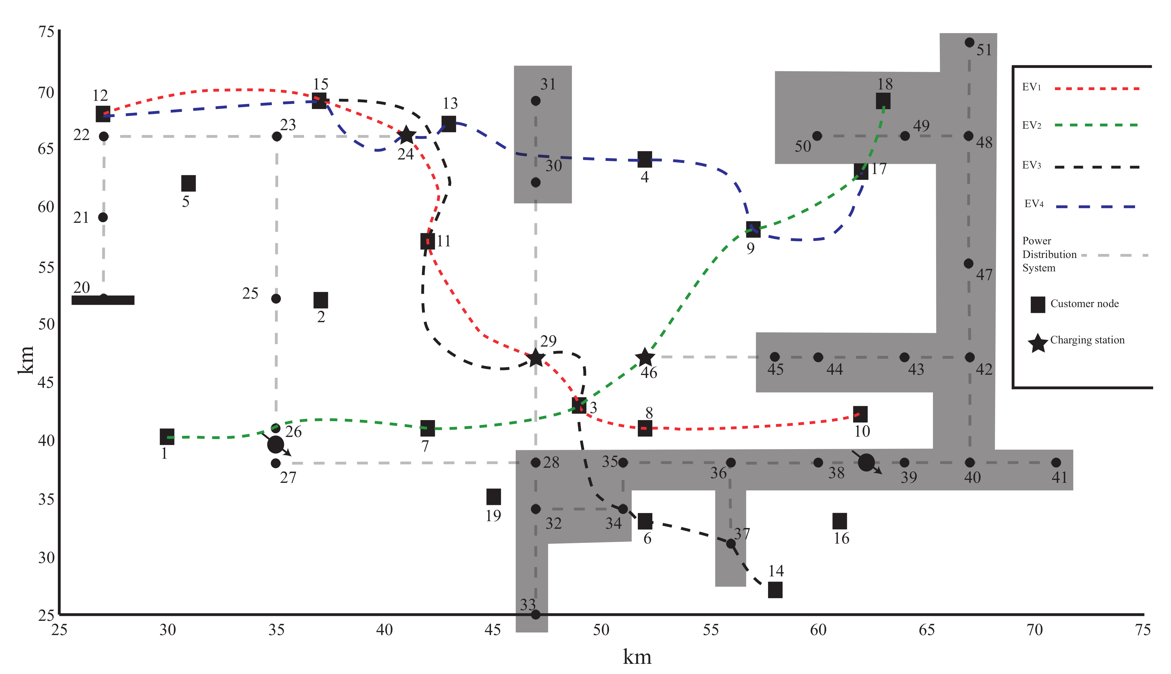
To demonstrate the sensitivity of the mathematical model, some of the power distribution network nodes are banned for charging station installation. We took the case for $Q_{CVRP}$ = 50 and $Q_{LMDP}$ = 28 and fix the variable $U_g$ = 0 to represent this ban, which is tagged in Table 1 with an asterisk. See in Figure 7 and Figure 8 the routes performed by the EVs in the CVRP and LMDP patterns, considering the shadow area that contains the power network nodes not allowed for installing charging stations.

Comparing the results from Figure 5 and Figure 6 with respect to Figure 7 and Figure 8, the routing cost for the CVRP is increased when some of the power network nodes are not allowed for charging station installation because this restriction makes the solution relocate the charging station that results in a larger route for the EV. Notice that a charging station had been installed at node 31; furthermore, incorporating the charging station install ban, this was relocated to node 24 as depicted in Figure 7. This situation can be seen with other charging stations that were relocated along the EV routes. Additionally, the number of charging stations is less, the increase in energy losses is reduced, and computational time reflects a significant decrease in comparison with the case of banned power network nodes. Although the objective function value is not decreased, the increment in this value is about 2%. This results in restricting power network nodes for installing charging stations, providing an improvement in finding a suitable solution, as part of a heuristic that can be initially run before executing the CPLEX solver.

Figure 9 presents an exponential tendency on the delta in energy losses with respect to the benchmark case solution, considering the change in battery capacity. Particularly, for the experiments $Q_{CVRP}=50$/$Q_{LMDP}=28$ and $Q_{CVRP}=60$/$Q_{LMDP}=32$, there is a decrease of 18% and 27%, respectively, in delta of energy losses, when the ban is applied for some of the electrical nodes. From the mathematical model standpoint, this is translated into a solution space curtailment, forcing the installation of charging stations at more attractive locations in terms of value for the objective function, which results in a suitable practice to initially run a heuristic as mentioned before.

5. Conclusions and Avenues of Research

In this study, the eLCVRP-CS-PDS is modeled via a mixed integer linear mathematical model, seeking feasible and good quality routes for light commercial EVs within the goods delivery operation to a fixed number of customers. Due to the charging station installation in order to make the EV routes completion suitable, the effect on the power distribution system is considered from the energy losses standpoint, through a linear power flow formulation supported by an affine constraint. A sensitivity analysis was performed by changing the battery capacity for the two patterns used throughout the routing, the first one accounting for the Capacitated Vehicle Routing Problem and the second one considered the Last Mile Delivery Problem using the shortest path approach. The change in battery capacity provides insights on the quantity and the more convenient location of charging stations along the distribution system that supports the decision maker in the grid future planning according to the current EV battery technology. Additionally, the energy consumed by the EVs and the increase in energy losses compared with the energy losses in the benchmark case were calculated. Other objectives such as the routing cost for the transportation patterns were also considered, reflecting a decrease in this objective as the battery capacity of the EVs was increased. Under this context and considering that there is a variation in energy losses with respect to charging station location, the computational experiments show that installing charging stations electrically closer to the substation results in a reduction of the energy losses. This was clearly observed when some of the power network nodes were banned for charging station installation. On the other hand, the newly designed three-index mathematical model within the routing formulation allowed multiple charging stations visits of EVs based on incoming and outgoing freight flow constraints at each node, without the need for using power network nodes copies, which may represent an increase in the computational complexity. The ban of installing charging stations at some power network nodes represents a suitable practice for finding good quality solutions in much less computational times, which can be translated into a heuristic context to obtain an initial solution for the CPLEX solver. Solving large sized-problems and NP-hard nature are still the traditional drawbacks that can be found in the eLCVRP-CS-PDS. Avenues of research may be focused on metaheuristic algorithms and developing heuristic methodologies based on solution space curtailment. With regard to the mathematical model, all of the realistic situations were not considered in this work that can be included in future research, such as multi depot vehicle routing problem, backhauls, and time window constraints.

Some final reflections are framed within the realistic approach that suggests independent owners for the power distribution and transportation networks. As depicted throughout this paper, it was assumed that both networks belong to the same owner, as the objective function involves electrical and routing components. Due to the managerial point of view and considering a single owner for both networks, an existing trade-off can be found between the terms in the objective function, contingent upon owner core business. This latter is related to goods transportation and delivery for a logistics company. For a power utility company, the core business is providing energy to homes and industrial customers. However, more utility companies are increasingly integrating logistic activities within their business, encouraging EV sales to logistics companies to increase the recharge of these vehicles by using their power grids.