A Set Covering Model for a Green Ship Routing and Scheduling Problem with Berth Time-Window Constraints for Use in the Bulk Cargo Industry

Abstract

This paper presents a set covering model based on route representation to solve the green ship routing and scheduling problem (GSRSP) with berth time-window constraints for multiple bulk ports. A bi-objective set covering model is constructed with features based on the minimization of the total CO₂ equivalent emissions and the total travel time subject to a limited number of berths in each port, berthing time windows, and the time window for each job. The solutions are obtained using the ε-constraint method, after which a Pareto frontier is plotted. This problem is motivated by the operations of feeder barges and terminals, where the logistics control tower is used to coordinate the routing and berthing time of its barges. We show that the proposed method outperforms the weighted sum method in terms of the number of Pareto solutions and the value of the hypervolume indicator.

1. Introduction

Inland waterway transportation (IWT) is a potential alternative that plays an important role in the transport of goods to every region of the world [1]. There are around 623,000 km of navigable waterways around the world [2], and as most of these are part of a river system, the network of rivers and river basins connects hundreds of cities and industrial areas. IWT is the most economical mode of inland transportation and an environmentally friendly alternative compared with other modes of transport [3,4]. In addition, it helps to reduce road congestion in densely populated regions. Bulk cargo is one of the most important cargo groups involved in inland waterway transportation, and it includes the carriage of bulk goods, such as coal, soil, rocks, cement, rice, sugar, and tapioca, among others.

Today, attention is focused on the continuously increasing environmental impact of air emissions, especially those from cargo ships [5]. The International Maritime Organization (IMO) [6] is expected to increase its emissions by 150–250% from 2012 to 2050 based on a business-as-usual scenario due to a tripling of world trade. This trend of emissions growth has resulted in proactive GHG management, which will be essential to enable the transportation industry to achieve its goal of limiting the effects of climate change [5,7,8]. A waterway transportation plan aimed at minimizing CO₂ emissions will reduce both air and water pollution, and also help to promote a positive image for environment conservation organizations.

In Thailand, bulk transportation is widely used on the Chao Phraya River. Over the years, many waterway transportation carriers and company-owned cargo terminals have attempted to collaborate to produce centralized decisions by employing a control tower to plan and control waterway transportation, reduce costs, and improve CO₂ emission efficiency. This control tower is responsible for integrating information and resources from all collaborative parties to solve the green ship routing and scheduling problem (GSRSP) as it applies to IWT. Another important consideration is that several often-contrasting objectives can be considered for the GSRSP. In the real world, most of them involve multiple objectives. Moreover, a control tower must focus on the berthing timeslots of each port when planning barge routes and schedules. We call this problem the green ship routing and scheduling problem (GSRSP) with berth time-window constraints (GSRSP-BT). Currently, decisions on ship routing and scheduling for IWT are made using a heuristic method, leading to non-optimal solutions and the provision of just one solution. Therefore, the control tower needs a high-performance technique that can solve the problem from a centralized decision-making position to obtain a Pareto frontier to make a decision tradeoff between the two objectives from that plot.

In this paper, we present a bi-objective set covering model based on route representation to solve the green ship routing and scheduling problem with berth time-window constraints (GSRSP-BT) for multiple bulk ports to minimize CO₂ equivalent (CO₂e) emissions and the total travel time, subject to the limited number of berths in each port, berthing time windows, and time window required for each job. We also plot a Pareto frontier using the ε-constraint method. In addition, we developed three constraints to specifically use with the proposed bi-objective set covering model based on route representation include (1) time window required for each job constraint, (2) time windows for each berth constraint, and (3) constraint to ensure that the berth does not serve more than one barge simultaneously.

The proposed method is applied to inland waterway shipping for dry bulk cargo on the Chao Phraya River, Thailand. The remainder of this paper is organized as follows. Section 2 reviews the related literature, Section 3 describes the components of the problem, Section 4 develops the proposed method, Section 5 reports the computational results, and Section 6 presents the conclusions.

2. Literature Review

2.1. Ship Routing and Scheduling Problems

For many decades, ship routing and scheduling problems (SRSP) have been a broad topic of research. In fact, a review of the research concerning ship routing and scheduling complications has been published roughly every 10 years. In the early 1980s, Ronen [9] reviewed the work in this field and then delivered a revised summary of correlated work in the field of SRSP from the 1980s and the 1990s ten years later [10]. Unfortunately, there has been little change to the shortage of articles in this area. Christiansen et al. [11] also examined research on ship scheduling and routing from a different perspective. Carrier collaboration, computer-aided decision support systems, software/hardware development, and supply chain management are a few of the trends that have emerged in recent decades. Christiansen et al. [12] published material from 2002 to 2011, and this is detailed in a recent summary of the SRSP. Four basic models used in this field were critically reviewed, and SRSP research trends were identified. We found that several studies had proposed several approaches to solve the SRSP decades ago.

Korsvik and Fagerholt [13] presented a tabu search heuristic method to solve the ship routing and scheduling problem with the transport of bulk products. The objective function maximizes the revenue for all cargo using the route. Korsvik et al. [14] proposed a large neighborhood search heuristic method for the ship routing and scheduling problem with split loads to maximize profit for bulk product transportation. Stålhane et al. [15] presented a branch-price-and-cut algorithm to solve a maritime pickup and delivery problem with time windows and split loads. The objective was to maximize the total profit. Kosmas and Vlachos [16] presented a simulated annealing-based algorithm to solve the ship routing problem to minimize cost. Nishi and Izuno [17] proposed a heuristic algorithm based on the column generation method to solve the ship routing and scheduling problem with split deliveries to minimize the total distance and satisfy the capacity of tankers. Lee and Byung-In Kim [18] formulated a mixed integer programming model for the industrial ship routing problem with split delivery to reduce the operation costs. An adaptive large neighborhood search-based heuristic model was proposed to solve the problem. De et al. [19] formulated a mixed integer non-linear programming model to solve the sustainable integrated dynamic ship routing and scheduling problem to reduce carbon emissions. They used particle swarm optimization with composite particles to solve the problem. Guan et al. [20] presented a fleet routing and scheduling problem with uncertain time window constraints. They solved the problem using the column generation optimization technique. Lin and Chang [21] proposed a Lagrangian relaxation-based decomposition algorithm to solve liner ship routing and freight assignment problems. Yamashita et al. [22] proposed a multi-start heuristic method for ship routing and scheduling by an oil company to minimize transportation costs and the number of consecutive dockings at platforms and terminals. Li [23] formulated a mixed integer programming model for a ship routing and scheduling problem for a steel plant cluster based alongside the Yangtze River. The proposed model was solved using an exact solution approach based on a dynamic programming algorithm.

2.2. Green Ship Routing and Scheduling Problem

The role of operations research (OR) in reducing air pollution from maritime and waterway transport will receive a lot more publicity in the coming years [5,12]. Potential avenues to incorporate air pollution aspects into maritime transportation OR were outlined by Christos and Kontovas [5]. As a result, more research-related greedy randomized adaptive search procedure (GRASP) has begun. Song et al. [24] developed a multi-objective model for the green vessel scheduling problem, where one of the objectives was to minimize the total CO₂ emissions and to generated the Pareto-optimal solutions using a multi-objective genetic algorithm. Dulebenets et al. [25] proposed a mathematical model for green vessel scheduling to minimize the total route service cost and solve the model using the CPLEX Optimizer. Dithmer et al. [26] presented the liner shipping routing and scheduling problem to minimize the external cost of ship air emissions. This entailed creating a schedule for a vessel to visit a fixed set of ports while minimizing costs and taking environmental factors into account. Dulebenets [27] developed a mixed-integer non-linear mathematical model for the green ship scheduling problem that directly accounts for CO₂ emission costs at sea and in ports of call. They linearized the original non-linear model to solve the problem using the CPLEX Optimizer. Cheaitou and Cariou [28] proposed a liner shipping multi-objective optimization model based on profit maximization and CO₂ emissions. Chen et al. [29] solved a green vehicle routing and scheduling problem with soft time windows using the design and improvement of an intelligent water drop algorithm. Zhen et al. [30] proposed a bi-objective mixed-integer linear programming model to optimize the sailing routes and speeds of liner ships considering emission control policies to minimize the total fuel cost and SO₂ emissions. The proposed problem was solved using a model that combined the two-stage iterative and fuzzy logic approaches based on the ε-constraint. Siahaan et al. [31] proposed a bin-packing problem to solve green-ship routing problems to minimize the total distribution cost for central parts of Indonesia and to minimize CO₂ emissions. Baykasog˘lu and Kemal Subulan [32] focused on reducing the overall cost of the intermodal transportation system, minimizing the total transit times and the total CO₂ emissions. They developed a mixed-integer mathematical programming model for a multi-objective sustainable load planning problem and solved the proposed model using a compromise programming approach. Wibisono and Jittamai [33] proposed a multi-objective evolutionary algorithm to solve a ship routing problem and generated Pareto optimal solutions while jointly minimizing total cost and deviation in fair cost proportion. Martínez-López et al. [34] identified the optimal sizing and the most adequate propulsion plant for a fleet of feeder vessels to minimize the total cost, the transportation time, and the environmental costs. They solved the problem and generated the Pareto front with an NSGA-II algorithm. Ma et al. [35] developed a multi-objective ship routing and speed model to minimize of shipping costs and emissions. They used a non-dominated sorting genetic algorithm II (NSGAII) to obtain the Pareto-optimal set, and the technique for order of preference by similarity to ideal Solution (TOPSIS) was used to find the trade-off solution from the Pareto-optimal set. Recently, Zhao et al. [36] proposed a hybrid multicriteria ship route planning method based on an improved particle swarm optimization and genetic algorithm generated in order to obtain the Pareto frontier and to make a decision tradeoff among the minimum navigation time route, fuel consumption route, navigation risk route.

In fact, most real-world problems have several objectives. Therefore, a multi-objective approach is essential to solving the GSRSP following the review of the literature mentioned above. This problem often has to be considered for different objectives, such as distance, time, emissions, profit, revenue, etc. [5] We found that most multi-objective approaches to solving the GSRSP focus on generating Pareto solutions by taking into account the trade-off among several objectives. The advantages of taking non-dominated solutions from Pareto fronts in the maritime transport applications are as follows:

The Pareto approach provides decision-makers (maritime regulators) with several alternative solutions associated with objective functions. It provides more choices for the decision-maker to consider and find the best balance among objectives based on their needs [33,37].

Maritime regulators can use the Pareto fronts to both make short-term decisions and devise long-term strategies to be defined based on the behavior of these frontiers [38].

This method is more realistic, particularly when decision-makers (maritime regulators) are undecided about the weights or when a trade-off relation among objective functions is not established a priori [33].

In addition, the selection of a unique optimal solution from a set of Pareto solutions, which results in less computational effort for the proposed multi-objective approach [32].

Based on this literature review and the merits of the Pareto fronts, most researchers offer various methods to obtain the Pareto fronts in maritime transport applications. However, it is clear that relatively few studies have investigated solutions for the green ship routing and scheduling problem (GSRSP), and no articles have studied the GSRSP with berthing time conditions (GSRSP-BT).

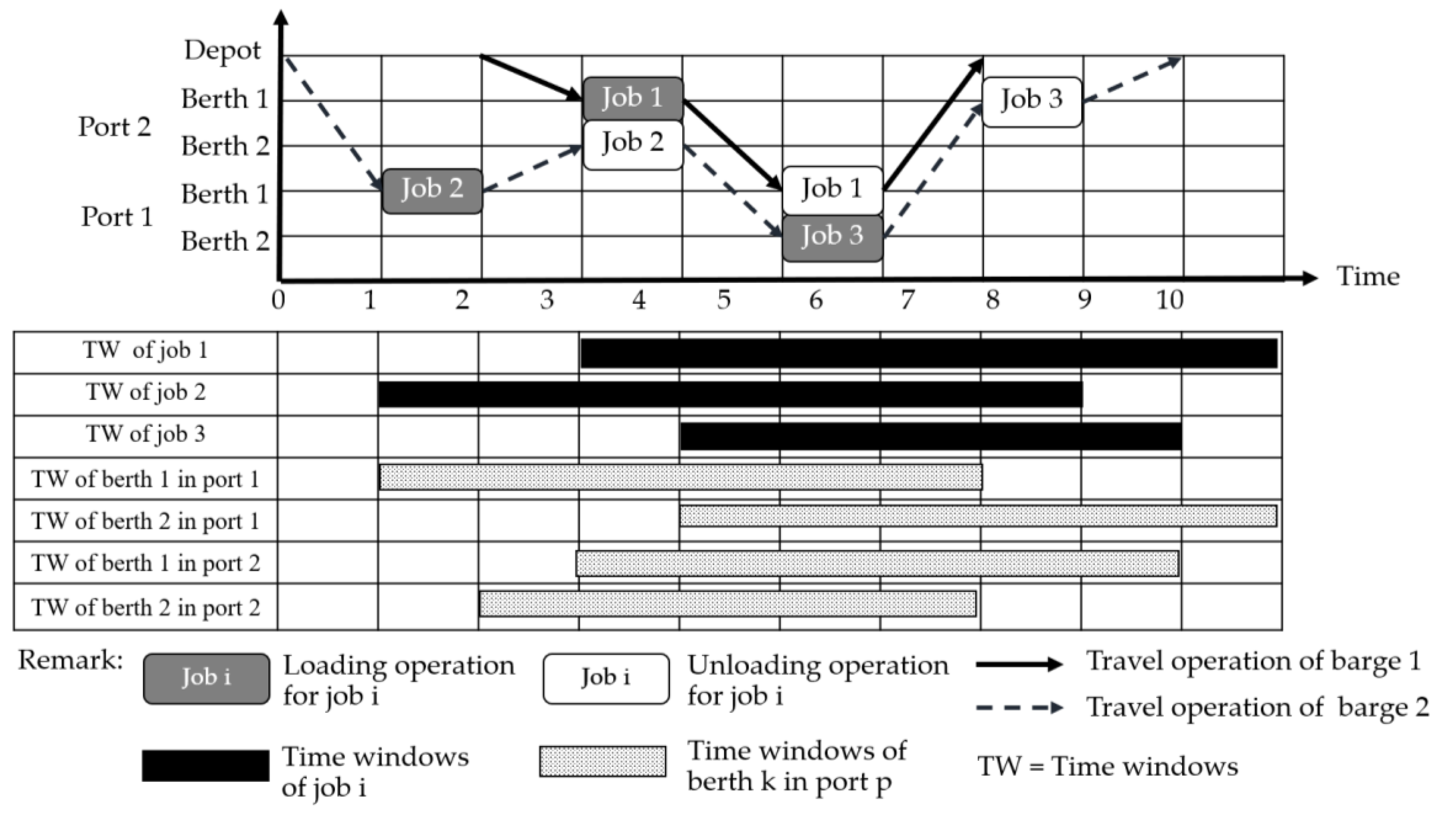
3. Problem Description

The green ship routing and scheduling problem with berth time window constraints (GSRSP-BT) addressed in this paper involves the routing of a fleet of controlled ships and the allocation of berth times to barges at the ports, subject to a limited number of berths in each port, berthing time windows, and the time window required for each job. A control tower is responsible for decisions and controls the private fleet and berthing time slots of each port while aiming to minimize the total CO₂ equivalent emissions and total travel time.

The barge type investigated in this research is dry bulk barge, which transports raw materials. A full barge load involves bulk cargo transportation; service providers have to move products between specified pairs of bulk port terminals with full barge loads. Barges travel from the depot to pick up and transport cargo from their origins to their destinations. There is a fleet of barges that return to the depot after completing all jobs. Cargo ships in Thailand have to return to the depot after serving all customers to prevent mooring outside of the port, which would obstruct the flow of the Chao Phraya River, which is the main drainage route from Northern Thailand to the sea during the flood season. However, the classical ship routing problem does not normally involve the return of ships to the depot. The bulk port terminal is divided into a specified number of berths (discrete layout), and it can serve as both an origin and a destination. When a barge is docked, the excavator loads the goods from the barge to trucks. After that, trucks transport the goods to the yard. Regarding the loading of goods onto the barge, trucks pick up goods from the yard, take them to the riverside, and then dump them onto the conveyor to transport them onto the ship. Each port terminal has a finite number of berths, and each berth is capable of serving (i.e., loading and unloading) one barge at a time, as shown in Figure 1. Additionally, berths have time windows during which the barges can be moored.

We refer to each pickup and delivery operation as a ‘‘job’’. We constructed two dummy jobs, i₀ and i_d, to represent the initial departure from a depot and the final arrival of barge v at the same depot, respectively. We pre-assigned barge v to handle dummy jobs i₀ and i_d, so that only barge v handles these two jobs. We let I′ denote the set of total jobs including jobs and dummy jobs (e.g., {0-job1-job2-job3-0}). We let I denote the set of all jobs (e.g., {job1-job2-job3}). This problem has P ports and k berths. Each job consists of a sequence of operations O_i,h. The execution of each operation h of a job i (noted as O_i,h) requires one port out of a set of given ports called P_i,h⊂P. Each port is independent of the others. The port setup time and the transfer time between operations are negligible. Examples of each operation of waterway transportation are presented in

Table 1. An example of each operation of waterway transportation.

Job (i)	Loading Operation (Oi,1)	Travel Operation (Oi,2)	Discharge Operation (Oi,2)
1	Port 2, Berth 1	Port 2 > Port 1	Port 1, Berth 1
2	Port 1, Berth 1	Port 1 > Port 2	Port 2, Berth 2
3	Port 1, Berth 2	Port 1 > Port 2	Port 2, Berth 1

.

We formulated the problem by establishing an underlying network with node set I as follows: between any two nodes i,j ∈ I, there are directed arcs i→j and j→i. Having barge v traverse arc i→j means that barge v handles both jobs, i and j, and it handles job i immediately before job j. Additionally, jobs have time windows in which barges can perform pickup and delivery operations for job i. The job time windows are set by the time when job i is ready (a_i) and the due date of job i (b_i), while service of job i must occur during the time windows of job i [a_i, b_i]. The berth time window is set based on the time when berth k is ready (r_k) and the latest allowed arrival time at berth k (l_k), while service at the loading node and discharge node of job i must occur during the time windows of the berth [r_k, l_k]. The depot also has a time window [a₀, b₀]. We assume that barges are allowed to wait at the river. Therefore, if barge v arrives at berth k before r_k and a_i, then it has to wait until berth k is ready for service and job i is ready for loading and unloading goods at berth k. All containers are assumed to be of the same size. The capacity of a barge is measured by the number of containers it can hold. However, the berths belonging to the same cargo terminal are assumed to have the same loading/unloading time and cost per container. In addition, each barge is allowed to occupy a berth only within a specific time window. It is unlikely for a barge to visit the same terminal multiple times during that period. Cargo is loaded in barges at a constant average rate. Barges have enough capacity to carry all of their assigned cargo. Barges sail at a specific constant speed. Barges have enough fuel to reach their destinations. The capacity of each barge is equal to the demands of job j.

We provide an example of a feasible solution to a problem concerning two barges that have to carry cargo for job numbers 1, 2, and 3 under the conditions of the capacity of each port time, the time window for each job, and the time window for each berth. An example of a feasible solution to the problem is presented in Figure 2. In Figure 2, the feasible route of a vehicle is described as follows: barge 1 departs from the depot and performs job 1 by loading the products of job 1 at berth 1 in port 2 within the time window of job 1 and the time window of berth 2 in port 1. Then, it unloads at berth 1 in port 1 within the time window of job 1 and the time window of that berth. Finally, barge 1 returns to the depot. This route sequence can be written in route format as {depot > port 2 > port 1 > depot} or in job sequence format as {depot > job1 > depot}.

4. Proposed Method

The objective of the proposed method is to find a feasible solution for the GSRSP-BT and to generate a Pareto frontier that can be used to make a decision tradeoff between the two objective functions. In the following text, we present the notations used in the proposed method:

Set
$R$	Set of feasible routes, $r\in R$
$P$	Set of ports, $p\in P$
Pv	Set of all ports used for job sequence numbers v in route r, pv ∈ Pv
$I$	Set of nodes, $i,j\in I$
Vr	Set of job sequence numbers on route r, v ∈ Vr
S	Set of periods, $s\in S$
Svp	Set of periods for job sequence v operated from port p, svp∈Svp
G	Set of the number of Pareto solutions, g ∈ G
K	Set of the number of berths, k ∈ K
Kp	Set of the number of berths in port p, kp ∈ Kp
Parameters
$\alpha$	Emission factor—fuel consumption per liter.
$\beta$	Emission factor for electricity consumption.
$E$	Electricity consumed.
${\tau }_{vs{k}_p}$	Binary parameter that takes a value of 1 if job sequence v allows the loading or unloading of goods at berth k in period s and a value of 0 otherwise.
${\mu }_{p_v}$	Binary parameter that takes a value of 1 if job sequence v must load or unload of goods in port p within the specified time window and a value of 0 otherwise.
${\omega }_{p_v}$	Binary parameter that takes a value of 1 if the completion time of job sequence v in route r at port p is within the specified time window and a value of 0 otherwise.
$n_{ri}$	The number of trips required for transport job i using route r.
${\mu }_v$	Binary parameter that takes a value of 1 if the start time of job sequence v in route r is within the time windows of job sequence v and a value of 0 otherwise.
${\omega }_v$	Binary parameter that takes a value of 1 if the completion time of job sequence v in route r is within the time windows of job sequence v and a value of 0 otherwise.
$e_{p_v}$	Earliest allowed arrival time for job sequence v operated in port p.
$l_{p_v}$	Latest allowed arrival time for job sequence v operated in port p.
$e_v$	Earliest allowed arrival time for job sequence v.
$l_v$	Latest allowed arrival time for job sequence v.
$s{t}_{p_v}^{load}$	Start time for loading products from job sequence v in port p.
$s{t}_{p_v}^{unload}$	Start time for unloading products from job sequence v in port p.
$c{t}_{p_v}^{load}$	Completion time for loading products from job sequence v in port p.
$c{t}_{p_v}^{unload}$	Completion time for unloading products from job sequence v in port p.
$c_{ij}$	The amount of fuel used when traveling from node i to node j.
$t_{ij}$	The travel time taken when traveling from node i to node j.
$t_i$	The service time at job i. Note that ti is dependent on the types of operation (either non-operation (job i is depot) or loading or unloading). where: $t_i=\{\begin{array}{l}0,\\ t_i^l,\\ t_i^u,\end{array}$$\begin{array}{l}\mathrm{i}\mathrm{f}\mathrm{n}\mathrm{o}\mathrm{n}-\mathrm{o}\mathrm{p}\mathrm{e}\mathrm{r}\mathrm{a}\mathrm{t}\mathrm{i}\mathrm{o}\mathrm{n}\mathrm{a}\mathrm{t}\mathrm{j}\mathrm{o}\mathrm{b}i\mathrm{a}\mathrm{n}\mathrm{d}\mathrm{j}\mathrm{o}\mathrm{b}i\mathrm{i}\mathrm{s}\mathrm{d}\mathrm{e}\mathrm{p}\mathrm{o}\mathrm{t}\\ \mathrm{i}\mathrm{f}\mathrm{l}\mathrm{o}\mathrm{a}\mathrm{d}\mathrm{i}\mathrm{n}\mathrm{g}\mathrm{o}\mathrm{p}\mathrm{e}\mathrm{r}\mathrm{a}\mathrm{t}\mathrm{i}\mathrm{o}\mathrm{n}\mathrm{o}\mathrm{n}\mathrm{l}\mathrm{y}\mathrm{a}\mathrm{t}\mathrm{j}\mathrm{o}\mathrm{b}i\\ \mathrm{i}\mathrm{f}\mathrm{un}\mathrm{l}\mathrm{o}\mathrm{a}\mathrm{d}\mathrm{i}\mathrm{n}\mathrm{g}\mathrm{o}\mathrm{p}\mathrm{e}\mathrm{r}\mathrm{a}\mathrm{t}\mathrm{i}\mathrm{o}\mathrm{n}\mathrm{o}\mathrm{n}\mathrm{l}\mathrm{y}\mathrm{a}\mathrm{t}\mathrm{j}\mathrm{o}\mathrm{b}i\end{array}$
$t_i^l$	Loading times at job i.
$t_i^u$	Unloading times at job i.
${\eta }_{s_{vp}}^{load}$	Binary parameter that takes a value of 1 if barge loading occurs at port p for transport job sequence v in route r in period s.
${\eta }_{s_{vp}}^{unload}$	Binary parameter that takes a value of 1 if barge unloading occurs at port p for transport job sequence v in route r in period s.
$K_{sp}$	The number of berths that are available in port p in period s.
N	The carrier’s maximum number of barges
$r_{k_p}$	Time at which berth k in port p is ready.
$l_{k_p}$	Latest allowed arrival time for berth k in port p.
Variables
$CO{E}_r$	The total CO2 equivalent emissions of route r.
$T{T}_r$	The total travel time for route r.
Decision variables
$y_{ij,r}$	1, if the barge traversed from job i to job j in route r. 0, otherwise.
$x_r$	1, if route r is selected. 0, otherwise.

The proposed method consists of two components: (a) the data preprocessing phase generates all feasible routes, as described in Section 4.1 and (b) the proposed set is solved using a model with a branch-and-cut algorithm and a Pareto frontier is generated using the ε-constraint method, as demonstrated in Section 4.2. A flowchart of the proposed method is shown in Figure 3.

4.1. Data Pre-Processing

A set of feasible routes and related parameters are first generated to solve the set covering model for the GSRSP-BT. In this step, all feasible routes for each barge are generated, and the parameters, including r, v, p_v, n_ri, y_ij,r, $s{t}_{p_v}^{load}$,$s{t}_{p_v}^{unload}$,$c{t}_{p_v}^{load}$,$c{t}_{p_v}^{unload}$, ${\eta }_{s_{vp}}^{load}$ and ${\eta }_{s_{vp}}^{unload}$, are defined. A feasible route is a barge travel sequence from the depot to other ports and then back to the same depot. Job sequences of route r are defined as v = {1, 2, …, Vr} and used as the indices of departure and arrival job sequence numbers on route r. P_v is defined as the set of all ports used in job sequences v on route r and p_v is the indices that define port of job sequences v of route r (p_v ∈ P_v, P_v ⊂ P). Therefore, each job sequence uses one port for loading and one port for unloading. As a result, Pv is a set of {1,2}. Note that job sequence 0 is the origin and destination depot. One example of a feasible route is given in Figure 4.

In this paper, we create all feasible routes in job sequence format. The data pre-processing steps are as follows:

Step 1: Use the backtracking algorithm developed by Maneengam and Udomsakdigool [39,40] to generate all feasible routes in job sequence format. Then, keep all feasible routes that satisfy constraints (1)–(5) as candidate routes.

$${\displaystyle \prod _{v\in V_r}{\displaystyle \prod _{p_v\in P_v}{\mu }_{p_v}}}\ge 1\forall r\in R$$

(1)

$${\displaystyle \prod _{v\in V_r}{\displaystyle \prod _{p_v\in P_v}{\omega }_{p_v}}}\ge 1\forall r\in R$$

(2)

$${\displaystyle \sum _{i\in I}{n}_{ri}=1\forall r\in R}$$

(3)

$${\displaystyle \prod _{v\in V_r}{\mu }_v}\ge 1\forall r\in R$$

(4)

$${\displaystyle \prod _{v\in V_r}{\omega }_v}\ge 1\forall r\in R$$

(5)

where

$${\mu }_{p_v}=\{\begin{array}{l}1,e_{p_v}\le \left(s{t}_{p_v}^{load}\wedge s{t}_{p_v}^{unload}\right)\le l_{p_v}\\ 0,Otherwise\end{array}$$

(6)

$${\omega }_{p_v}=\{\begin{array}{l}1,e_{p_v}\le \left(c{t}_{p_v}^{load}\wedge c{t}_{p_v}^{unload}\right)\le l_{p_v}\\ 0,Otherwise\end{array}$$

(7)

$${\mu }_v=\{\begin{array}{l}1,e_v\le \left(s{t}_{p_v}^{load}\wedge s{t}_{p_v}^{unload}\right)\le l_v\\ 0,Otherwise\end{array}$$

(8)

$${\omega }_v=\{\begin{array}{l}1,e_v\le \left(c{t}_{p_v}^{load}\wedge c{t}_{p_v}^{unload}\right)\le l_v\\ 0,Otherwise\end{array}$$

(9)

Constraint (1) ensures that the start time of job sequence v of route r and using port p is within the specified time windows of port p_v. Constraint (2) ensures that the completion time of job sequence v using route r and port p is within the specified time windows of port p_v. Constraint (3) ensure that each job is used exactly once for all routes. Constraints (4) and (5) ensure that the start and completion times of job sequence v using route r are within the time windows of job sequence v. Equations (6) and (7) determine the binary parameters to describe whether ${\mu }_{p_v}$ and ${\omega }_{p_v}$ = 1 mean that the start and completion times at port p_v within its time windows are satisfied. Otherwise, they are set to 0, and these binary parameters are used in constraints (1) and (2), respectively. Therefore, Equations (8) and (9) determine the binary parameters to describe whether ${\mu }_v$ and ${\omega }_v$ = 1 mean that the start and completion times at port p_v within the time window of job sequence v are satisfied. Otherwise, they are set to 0, and these binary parameters are used in constraints (4) and (5). The rest are removed.

Step 2: Define all feasible routes as the set of routes {r = 1,2, 3, …, R}.

Step 3: Calculate CO₂e emissions and total travel time for route r for all candidate routes as a parameter in the set covering model, as shown in Equations (10) and (11). We calculated the CO₂e emissions from the emission factors of transportation types based on an estimation method and on emission factors [41] in accordance with the Thailand Greenhouse Gas Management Organization (TGO) criteria.

$$CO{E}_r=\left[{\displaystyle \sum _{i,j\in I}{c}_{ij}{y}_{ij,r}}\right]\alpha +\left[\underset{v\in V_r}{\max }(c{t}_{p_v}^{unload})-\underset{v\in V_r}{\min }\left(s{t}_{p_v}^{load}\right)\right]E\times \beta$$

(10)

$$T{T}_r={\displaystyle \sum _{i,j\in I}{t}_{ij}{y}_{ij,r}}+{\displaystyle \sum _{i\in I}\left[t_i\left({\displaystyle \sum _{j\in I}{y}_{ij,r}}\right)\right]}$$

(11)

After completing pre-processing, as described in Section 4.1, the set of all candidate routes (r ∈ R), parameters of candidate route r, CO₂e emissions, and total travel time for route r are obtained and used as input parameters to solve the set covering model.

4.2. Solving the Proposed Set Covering Model

Typically, the classical GSRSP-BT model is quite difficult to solve directly via exact methods. The classical model must be reformulated into a set covering model that can find the route within a specified time window to allow possible solutions to be found with faster computational times. This problem has two objective functions: to minimize the total amount of CO₂e emissions and to minimize the total travel time. S is defined as a set of time periods (s ∈ S) and S_vp is a set of time periods for job sequence v operating in port p (s_vp ∈ S_vp, S_vp ⊂ S). The model assumes that the travel times and service times are the same in each period. In this step, we developed the port capacity constraint to avoid time clashes when barge loading and unloading in port p in period s using binary parameters ${\eta }_{s_{pv}}^{load}$ and ${\eta }_{s_{pv}}^{unload}$ for multiple berths in a port. The proposed set covering model is as follows:

$$Minimize{f}_1={\displaystyle \sum _{r\in r}CO{E}_r{x}_r}$$

(12)

$$Minimize{f}_2={\displaystyle \sum _{r\in R}T{T}_r{x}_r}$$

(13)

subject to

$${\displaystyle \sum _{r\in R}{x}_r{n}_{ri}}=1\forall i\in I$$

(14)

$${\displaystyle \sum _{r\in R}{x}_r}\le N$$

(15)

$${\displaystyle \sum _{r\in R}{\displaystyle \sum _{v\in V_r}{x}_r{\eta }_{s_{vp}}^{load}}}+{\displaystyle \sum _{r\in R}{\displaystyle \sum _{v\in V_r}{x}_r{\eta }_{s_{vp}}^{unload}}}\le K_{sp}\forall p\in P,\forall s_{vp}\in S_{vp},\forall s\in S$$

(16)

$$x_r\in \left\{0,1\right\}\forall r\in R$$

(17)

where

$${\eta }_{s_{pv}}^{load}=\{\begin{array}{l}1,\left(s{t}_{p_v}^{load}\right)\le s_{vp}\le \left(c{t}_{p_v}^{load}\right)\\ 0,Otherwise\end{array}$$

(18)

$${\eta }_{s_{pv}}^{unload}=\{\begin{array}{l}1,\left(s{t}_{p_v}^{unload}\right)\le s_{vp}\le \left(c{t}_{p_v}^{unload}\right)\\ 0,Otherwise\end{array}$$

(19)

$$K_{sp}={\displaystyle \sum _{k_p\in K_p}{\displaystyle \sum _{v\in V_r}{\tau }_{vs{k}_p}}}\forall p\in P,\forall s\in S$$

(20)

$${\tau }_{vs{k}_p}=\{\begin{array}{l}1,r_{k_p}\le s_{vp}\le l_{k_p}\\ 0,Otherwise\end{array}$$

(21)

Equations (12) and (13) are objective functions that are intended to minimize the total CO₂e emissions and the total travel time. Constraint (14) enables the formation of a transportation plan to transport goods according to the requirements of job i. Constraint (15) ensures that the number of barges used does not exceed the carrier’s maximum number of barges. Constraint (16) ensures that the total number of shipments specified at port p for loading and unloading does not exceed the loading capacity of port p (the number of berths in port p in period s) in period s. We developed this constraint for use specifically with the proposed bi-objective set covering model based on route representation. Constraint (17) ensures that the decision variable is binary valued. Equations (18) and (19) determine the binary parameter used to describe period s when the barge is docked at port p for transport job sequence v in route r. Equations (20) and (21) determine binary parameters (${\eta }_{s_{pv}}^{load}$ and ${\eta }_{s_{pv}}^{unload}$) that take a value of 1 if barge loading/unloading occurs at port p for transport job sequence v in route r in period s, and these binary parameters are used in constraint (16). The binary parameter $\left(s_{pv}\right)$ is obtained from the feasible route generation. The Pareto frontier is gained using the ε-constraint method proposed by Chankong and Haimes [42], which includes the following steps.

4.2.1. Solving the Single Objective Set Covering Model

Once the set of feasible routes R resulting from the process described in Section 4.1 is constructed, the single objective set covering model is solved by a branch-and-cut algorithm using Equation (12) and constraint sets (14)–(17). Similarly, by solving the model sharing the same constraint sets and taking Equation (13) as the objective, this step gives the optimal values of the two objectives denoted by f₁* and f₂*.

4.2.2. Setting the Number of Pareto Solutions

Decision-makers will first set the number of Pareto solutions that they want to obtain. G denotes the number of Pareto solutions. To generate Pareto solution g where g = 1,2,...,G, in this article, we define the number of Pareto solutions (G) as 10.

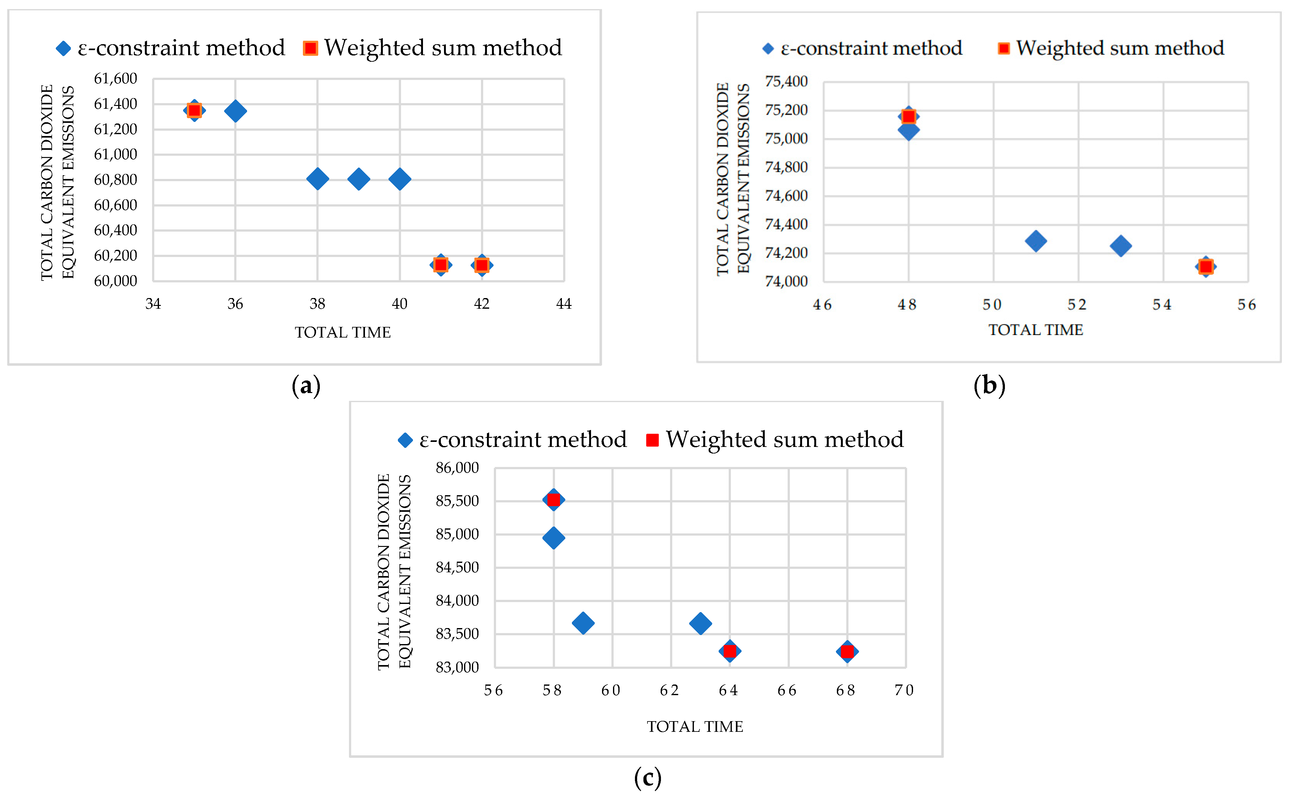
4.2.3. Plotting a Pareto Frontier

To optimize one of the objective functions m from two objectives, as shown in (18), the other objective functions are converted to constraints with fixed threshold values for constrained objective function z (ε_z) with z ∈ Z, z ≠ m, as shown in Equation (19). Therefore, the GSRSP-BT is replaced by the ε-constraint problem:

$$\underset{x\in X}{\min }{f}_m(x)$$

(22)

subject to

$$f_z(x)\le {\epsilon }_{z}z\in Z,z\ne m$$

(23)

where x is the vector of the decision variables. Pareto solutions can be obtained by variations in parameters in the RHS of constrained objective functions (ε_z).

5. Results

In this paper, the proposed method was applied to solve the real problem of dry bulk cargo transport on the Chao Phraya River and the anchorage area in the Gulf of Thailand, Thailand. This method was divided into two components: (1) Data pre-processing coded with JavaScript in NetBeans IDE 8.1 was applied to generate routes using the backtracking algorithm. (2) The proposed set covering model was solved using the branch-and-cut algorithm in OpenSolver 2.9.0 with the default settings. The experiments were run on a PC with an Intel^® Core™ i7-6800K CPU 3.40 GHz and 16 GB RAM.

The instances and parameters collected from February to May 2020 can be downloaded from https://sites.google.com/site/transportationlibrary (accessed on 20 May 2021). There is a total of 10 nodes in this problem, consisting of nine nodes on the river port and 1 node for the load discharge area, as shown in Figure 5. The location of each node is shown in

Table 2. Location of each node.

Location	Latitude, Longitude	Ready Time	Latest Allowed Arrival Time
1	(13.4735585, 100.98346600000002)	1	17
2	(13.6305239, 100.54398190000006)	2	17
3	(13.5234748, 100.26317930000005)	3	18
4	(14.0266045, 100.54322920000004)	4	20
5	(14.2508489, 100.58231790000002)	2	19
6	(14.3180176, 100.56809569999996)	1	17
7	(14.4157881, 100.59332919999997)	2	18
8	(14.4111553, 100.59306560000005)	3	18
9	(14.4772767, 100.6218513)	3	18
10	(13.140878, 100.823247)	0	100

.

In the case studies, each job transported 4000 tons, a volume equal to the capacity of a barge, and each river port had two berths that could operate in parallel. Three real-life instances were tested, as displayed in

Table 3. Configuration of testing instances.

Testing Instances	Number of Jobs (i)	Source > Destination	Ready Time of Job i–Latest Allowed Arrival Time of Job i
1	6	8 > 10, 10 > 8, 10 > 5, 10 > 2, 9 > 10, 7 > 10	2–18 5–17, 1–20, 3–20, 1–20, 3–20
2	8	8 > 10, 10 > 6, 10 > 9, 7 > 10, 8 > 10, 10 > 2, 10 > 1, 5 > 10,	1–17, 2–15, 3–16, 2–20, 3–17, 1–20, 4–15, 2–20
3	9	10 > 8, 7 > 10, 10 > 2, 10 > 3, 5 > 10, 10 > 8, 4 > 10, 10 > 6, 1 > 9,	1–20, 4–17, 3–18, 5–17, 1–19, 4–18, 2–19, 3–18, 4–17

.

Currently, decisions are made concerning ship routing and scheduling for IWT using a heuristic method based on the experience of the planning department staff. The old method where the author obtained information from the case study was able to find only one solution for three testing instances, as shown in

Table 4. Result obtained from old method for 3 testing instances.

Testing Instances	1f1	2f2
1	64,427.55	55
2	74,107.45	55
3	83,244.64	68

¹f₁ = The total CO₂e emissions (kgCO₂e), ² f₂ = The total travel time (days).

.

In this paper, we present the Pareto solutions obtained from the proposed method, and these are compared with the Pareto solutions obtained from the weighted sum method, as shown in

Table 5. The non-dominated solutions obtained from the ε-constraint method and the weighted sum method.

Testing Instances	NO.	2f2	1f1 Obtained from the ε-Constraint Method	1f1 Obtained from the Weighted Sum Method
	1	35	61,350.20	61,350.20
	2	36	61,346.93	-
	3	38	60,811.46	-
1	4	39	60,808.19	-
	5	40	60,808.19	-
	6	41	60,129.29	60,129.29
	7	42	60,126.02	60,126.02
	1	48	75,159.00	75,159.00
	2	48	75,065.19	-
2	3	51	74,287.01	-
	4	53	74,251.77	-
	5	55	74,107.43	74,107.43
	1	58	85,523.51	85,523.51
	2	58	84,947.72	-
	3	59	83,668.38	-
3	4	63	83,661.00	-
	5	64	83,249.36	83,249.36
	6	68	83,241.98	83,241.98

¹f₁ = the total CO₂e emissions (kgCO₂e), ² f₂ = the total travel time (days).

. Each method was run 10 times to obtain non-dominated solutions. The weights of the weighted sum method were adjusted 10 times, with each adjustment ranging from 0 to 1 and totaling a value of 1 exactly. The Pareto frontier or tradeoff between the total CO₂e emissions (f₁) and the total travel time (f₂) obtained with each method was plotted, as shown in Figure 6.

As shown in Table 5 and Figure 6, we found that the proposed method using the ε-constraint method provided more Pareto solutions than the weighted sum method for all instances, namely four, three, and three, respectively. The Pareto frontier clearly indicates that an increase in the total CO₂e emissions (f₁) will lead to a decrease in the total travel time (f₂). For example, if the customer and the carrier agree that the total CO₂e emissions should not exceed 84,000 kgCO₂e for transportation in testing instance 3, then the decision-makers can plan the transportation scheme using the third Pareto solution because it is the lowest total travel time under carbon emission conditions set by the agreement. Moreover, when comparing the Pareto solutions provided by the proposed method with the results provided by the old method, it was shown that the non-dominated solutions obtained using the proposed method were more effective than those obtained using the old method in both objectives for all testing instances.

Our analysis used the hypervolume indicator and the number of Pareto solutions found to measure the proposed method’s effectiveness, as shown in

Table 6. The hypervolume indicator of each method.

Testing Instances	1 HVe	2 HVw	HVe-HVw
1	58.51%	46.68%	11.82%
2	58.61%	13.47%	45.14%
3	85.92%	49.94%	35.97%

¹ HVe = the hypervolume indicator of ε-constraint method, ² HVw = the hypervolume indicator of weighted sum method.

. The hypervolume indicator is the area of all rectangular combinations. The larger the value of the hypervolume indicator (area), the better the set of solutions [43].

According to the hypervolume indicator [43] of both methods as shown in Table 6, the ε-constraint method represents a larger area than the weighted sum method for all instances: 11.82%, 45.14%, and 35.97%, respectively. The experimental results show that the ε-constraint method is more effective than the weighted sum method, consistent with previous studies that have compared the two methods [44,45]. Because of this, the ε-constraint method has better coverage for both objectives [45].

6. Conclusions

In this paper, a method to solve the GSRSP-BT while minimizing the total CO₂ equivalent emissions and the total travel time is presented. This problem includes finding the ship route and berthing time for each barge to perform loading/unloading operation to avoid time clashes for multiple ports in the bulk cargo industry. The proposed method has two components: (1) A backtracking algorithm is used to create all feasible routes with time windows for each job and for each port. These restrictions serve to screen feasible routes within the various time windows in consideration of the proposed bi-objective set covering model. (2) The proposed bi-objective set covering model is solved using a branch-and-cut algorithm, and the Pareto frontier is generated using the ε-constraint method while jointly minimizing the total CO₂e emissions and the total travel time objectives. In general, the mathematical model to solve this problem is quite difficult to solve it directly via exact methods. Therefore, we present a set covering model that reformulates the constraints to be easier to solve the GSRSP-BT. These constraints have been developed specifically for use with the proposed bi-objective set covering model based on route representation. We outline three testing instances from a real case study of a small company conducting transport using barges in the Gulf of Thailand and the Chao Phraya River.

According to the Pareto frontier obtained from the proposed method, an increase in total CO₂e emissions lead to a decrease in total travel time. The proposed method could offer various alternatives to control tower (decision-makers) using the Pareto frontier to make decisions and provide an appropriate transportation plan. Decision-makers can choose one of the Pareto solutions as routes and schedules for each barge based on the Pareto frontier to balance the two conflicting objectives at the same time [46]. The comparison of different bi-objective optimization methods shows that the proposed method can generate a variety of different Pareto solutions than the weighted sum method and the proposed method represents a larger value of the hypervolume indicator than the weighted sum method for all instances: 11.82%, 45.14%, and 35.97%, respectively. Moreover, all non-dominated solutions from the Pareto fronts produce better results than the old method for both the total CO₂e emissions and the total travel time due to the old method using the heuristic method, which primarily relies on employee routing and scheduling capabilities, which cannot guarantee the quality of solutions. It is clear that the proposed method can be used in real case studies in the Chao Phraya River instead of the old method, which offers only one solution. The Pareto fronts obtained from the proposed method also allow for long-term decisions based on the behavior of these boundaries when conducting a sensitivity analysis. In addition, the proposed bi-objective set covering model can be formulated in spreadsheets and easily integrated with solver software packages, making it easier to implement in real cases. We expect the proposed method to be a problem-solving tool for carriers or control towers looking for an easy and effective approach to solve the GSRSP-BT and causing them to account for environmental impact.

One of the limitations of this study is that the data pre-processing requires more space to store all feasible routes as the scale of the problem grows. For this reason, the proposed method does not solve large-sized instances, as the feasible route storage space is limited. In the future, we will develop a new method that can more effectively solve large-size instances of the GSRSP-BT and generate more comprehensive Pareto solutions. The author will increase the objective function of minimizing the navigation risk, which has been affected by an accident that may occur during the trip, water-way traffic jams, and the risk of cranes breakdown. Moreover, the travel time uncertainty will be taken into account to create a model which is as realistic and efficient as possible.

References

1. Li, Y. Application of New Technologies and Quality Standards System to Improve River Ship Officers’ Education and Training; World Maritime University: Malmö, Sweden, 1999. [Google Scholar]
2. Beyer, A. Inland Waterways, Transport Corridors and Urban Waterfronts Discussion Paper; Organisation for Economic Co-operation and Development: Paris, France, 2018. [Google Scholar]
3. NESDB. NESDB Economic Report; NESDB: Bangkok, Thailand, 2018. [Google Scholar]
4. UNCTAD. Review of Maritime Transport; UNCTAD: New York, NY, USA, 2018. [Google Scholar]
5. Kontovas, C.A. The Green Ship Routing and Scheduling Problem (GSRSP): A conceptual approach. Transp. Res. Part D Transp. Environ. 2014, 31, 61–69. [Google Scholar] [CrossRef]
6. Buhaug, Ø.; Corbett, J.; Endresen, Ø.; Eyring, V.; Faber, J.; Hanayama, S.; Lee, D.; Lindstad, E.; Markowska, A.Z.; Mjelde, A.; et al. Second IMO GHG Study 2009; The International Maritime Organization: London, UK, 2009. [Google Scholar]
7. Maneengam, A. A Bi-Objective Programming Model for Multimodal Transportation Routing Problem of Bulk Cargo Transportation. In Proceedings of the 2020 IEEE 7th International Conference on Industrial Engineering and Applications (ICIEA), Bangkok, Thailand, 16–18 April 2020; pp. 890–894. [Google Scholar]
8. Bouman, E.A.; Lindstad, E.; Rialland, A.I.; Strømman, A.H. State-of-the-art technologies, measures, and potential for reducing GHG emissions from shipping—A review. Transp. Res. Part D Transp. Environ. 2017, 52, 408–421. [Google Scholar] [CrossRef]
9. Ronen, D. Cargo ships routing and scheduling: Survey of models and problems. Eur. J. Oper. Res. 1983, 12, 119–126. [Google Scholar] [CrossRef]
10. Ronen, D. Ship scheduling: The last decade. Eur. J. Oper. Res. 1993, 71, 325–333. [Google Scholar] [CrossRef]
11. Christiansen, M.; Fagerholt, K.; Ronen, D. Ship Routing and Scheduling: Status and Perspectives. Transp. Sci. 2004, 38, 1–18. [Google Scholar] [CrossRef]
12. Christiansen, M.; Fagerholt, K.; Nygreen, B.; Ronen, D. Ship routing and scheduling in the new millennium. Eur. J. Oper. Res. 2013, 228, 467–483. [Google Scholar] [CrossRef]
13. Korsvik, J.E.; Fagerholt, K.; Laporte, G. A tabu search heuristic for ship routing and scheduling. J. Oper. Res. Soc. 2010, 61, 594–603. [Google Scholar] [CrossRef]
14. Korsvik, J.E.; Fagerholt, K.; Laporte, G. A large neighbourhood search heuristic for ship routing and scheduling with split loads. Comput. Oper. Res. 2011, 38, 474–483. [Google Scholar] [CrossRef]
15. Stålhane, M.; Andersson, H.; Christiansen, M.; Cordeau, J.F.; Desaulniers, G. A branch-price-and-cut method for a ship routing and scheduling problem with split loads. Comput. Oper. Res. 2012, 39, 3361–3375. [Google Scholar] [CrossRef]
16. Kosmas, O.T.; Vlachos, D.S. Simulated annealing for optimal ship routing. Comput. Oper. Res. 2012, 39, 576–581. [Google Scholar] [CrossRef] [Green Version]
17. Nishi, T.; Izuno, T. Column generation heuristics for ship routing and scheduling problems in crude oil transportation with split deliveries. Comput. Chem. Eng. 2014, 60, 329–338. [Google Scholar] [CrossRef]
18. Lee, J.; Kim, B.I. Industrial ship routing problem with split delivery and two types of vessels. Expert Syst. Appl. 2015, 42, 9012–9023. [Google Scholar] [CrossRef]
19. De, A.; Mamanduru, V.K.R.; Gunasekaran, A.; Subramanian, N.; Tiwari, M.K. Composite particle algorithm for sustainable integrated dynamic ship routing and scheduling optimization. Comput. Ind. Eng. 2016, 96, 201–215. [Google Scholar] [CrossRef]
20. Guan, F.; Peng, Z.; Chen, C.; Guo, Z.; Yu, S. Fleet routing and scheduling problem based on constraints of chance. Adv. Mech. Eng. 2017, 9, 1–12. [Google Scholar] [CrossRef] [Green Version]
21. Lin, D.Y.; Chang, Y.T. Ship routing and freight assignment problem for liner shipping: Application to the Northern Sea Route planning problem. Transp. Res. Part E: Logist. Transp. Rev. 2018, 110, 47–70. [Google Scholar] [CrossRef]
22. Yamashita, D.; da Silva, B.J.V.; Morabito, R.; Ribas, P.C. A multi-start heuristic for the ship routing and scheduling of an oil company. Comput. Ind. Eng. 2019, 136, 464–476. [Google Scholar] [CrossRef]
23. Li, F.; Yang, D.; Wang, S.; Weng, J. Ship routing and scheduling problem for steel plants cluster alongside the Yangtze River. Transp. Res. Part E: Logist. Transp. Rev. 2019, 122, 198–210. [Google Scholar] [CrossRef]
24. Song, D.-P.; Li, D.; Drake, P. Multi-objective optimization for planning liner shipping service with uncertain port times. Transp. Res. Part E: Logist. Transp. Rev. 2015, 84, 1–22. [Google Scholar] [CrossRef]
25. Dulebenets, M.A.; Golias, M.M.; Mishra, S. The green vessel schedule design problem: Consideration of emissions constraints. Energy Syst. 2017, 8, 761–783. [Google Scholar] [CrossRef]
26. Dithmer, P.; Reinhardt, L.; Kontovas, C.A. The Liner Shipping Routing and Scheduling Problem Under Environmental Considerations: The Case of Emissions Control Areas BT—Computational Logistics. In Proceedings of the 8th International Conference (ICCL), Southampton, UK, 18–20 October 2017; pp. 336–350. [Google Scholar]
27. Dulebenets, M.A. The green vessel scheduling problem with transit time requirements in a liner shipping route with Emission Control Areas. Alex. Eng. J. 2018, 57, 331–342. [Google Scholar] [CrossRef]
28. Cheaitou, A.; Cariou, P. Greening of maritime transportation: A multi-objective optimization approach. Ann. Oper. Res. 2019, 273, 501–525. [Google Scholar] [CrossRef]
29. Chen, G.; Wu, X.; Li, J.; Guo, H. Green vehicle routing and scheduling optimization of ship steel distribution center based on improved intelligent water drop algorithms. Math. Probl. Eng. 2020, 2020. [Google Scholar] [CrossRef]
30. Zhen, L.; Hu, Z.; Yan, R.; Zhuge, D.; Wang, S. Route and speed optimization for liner ships under emission control policies. Transp. Res. Part C: Emerg. Technol. 2020, 110, 330–345. [Google Scholar] [CrossRef]
31. Siahaan, J.J.A.; Pratiwi, E.; Setyorini, P.D. Study of Green-Ship Routing Problem (G-VRP) Optimization for Indonesia LNG Distribution. IOP Conf. Ser. Earth Environ. Sci. 2020, 557. [Google Scholar] [CrossRef]
32. Baykasoğlu, A.; Subulan, K. A multi-objective sustainable load planning model for intermodal transportation networks with a real-life application. Transp. Res. Part E Logist. Transp. Rev. 2016, 95, 207–247. [Google Scholar] [CrossRef]
33. Wibisono, E.; Jittamai, P. Multi-objective evolutionary algorithm for a ship routing problem in maritime logistics collaboration. Int. J. Logist. Syst. Manag. 2017, 28, 225. [Google Scholar] [CrossRef]
34. Martínez-López, A.; Caamaño Sobrino, P.; Chica González, M.; Trujillo, L. Optimization of a container vessel fleet and its propulsion plant to articulate sustainable intermodal chains versus road transport. Transp. Res. Part D Transp. Environ. 2018, 59, 134–147. [Google Scholar] [CrossRef]
35. Ma, W.; Ma, D.; Ma, Y.; Zhang, J.; Wang, D. Green maritime: A routing and speed multi-objective optimization strategy. J. Clean. Prod. 2021, 305, 127179. [Google Scholar] [CrossRef]
36. Zhao, W.; Wang, Y.; Zhang, Z.; Wang, H. Multicriteria ship route planning method based on improved particle swarm optimization–genetic algorithm. J. Mar. Sci. Eng. 2021, 9, 357. [Google Scholar] [CrossRef]
37. De, A.; Choudhary, A.; Tiwari, M.K. Multiobjective Approach for Sustainable Ship Routing and Scheduling with Draft Restrictions. IEEE Trans. Eng. Manag. 2019, 66, 35–51. [Google Scholar] [CrossRef] [Green Version]
38. Martínez-López, A. A multi-objective mathematical model to select fleets and maritime routes in short sea shipping: A case study in Chile. J. Mar. Sci. Technol. 2020, 1–20. [Google Scholar] [CrossRef]
39. Maneengam, A.; Udomsakdigool, A. Solving the collaborative bidirectional multi-period vehicle routing problems under a profit-sharing agreement using a covering model. Int. J. Ind. Eng. Comput. 2020, 11, 185–200. [Google Scholar] [CrossRef]
40. Maneengam, A.; Udomsakdigool, A. Solving the Bidirectional Multi-Period Full Truckload Vehicle Routing Problem with Time Windows and Split Delivery for Bulk Transportation Using a Covering Model. In Proceedings of the 2018 IEEE International Conference on Industrial Engineering and Engineering Management (IEEM), Bangkok, Thailand, 16–19 December 2018; pp. 798–802. [Google Scholar]
41. TGO (Thailand Greenhouse Gas Management Organization) Update Emission Factor CFP. Available online: http://thaicarbonlabel.tgo.or.th/admin/uploadfiles/emission/ts_822ebb1ed5.pdf (accessed on 20 January 2021).
42. Chankong, V.; Haimes, Y.Y. Multiobjective Decision Making: Theory and Methodology; North-Holland/Elsevier Science Publishing Company, Inc.: New York, NY, USA, 1983; ISBN 0444007105. [Google Scholar]
43. Friedrich, T.; Horoba, C.; Neumann, F. Multiplicative approximations and the hypervolume indicator. In Proceedings of the 11th Annual Genetic and Evolutionary Computation Conference (GECCO-2009), Montreal, QC, Canada, 8–12 July 2009; pp. 571–578. [Google Scholar] [CrossRef]
44. Chiandussi, G.; Codegone, M.; Ferrero, S.; Varesio, F.E. Comparison of multi-objective optimization methodologies for engineering applications. Comput. Math. Appl. 2012, 63, 912–942. [Google Scholar] [CrossRef] [Green Version]
45. Demir, E.; Hrušovský, M.; Jammernegg, W.; Van Woensel, T. Green intermodal freight transportation: Bi-objective modelling and analysis. Int. J. Prod. Res. 2019, 57, 6162–6180. [Google Scholar] [CrossRef] [Green Version]
46. Zhao, Y.; Fan, Y.; Zhou, J.; Kuang, H. Bi-objective optimization of vessel speed and route for sustainable coastal shipping under the regulations of emission control areas. Sustainability 2019, 11, 6281. [Google Scholar] [CrossRef] [Green Version]
Figure 1. Example of 2 berths in a port.
Applsci 11 04840 g001
Figure 2. Feasible solution for the example.
Applsci 11 04840 g002
Figure 3. A flowchart of the proposed method.
Applsci 11 04840 g003
Figure 4. Feasible route for the example.
Applsci 11 04840 g004
Figure 5. Locations of the river port and the anchorage area under study.
Applsci 11 04840 g005
Figure 6. All Pareto solutions: (a) the Pareto frontier of instance 1; (b) the Pareto frontier of instance 2; (c) the Pareto frontier of instance 3.
Applsci 11 04840 g006