Research on 3D Improved Extended Finite Element Method for Electric Field of Liquid Nitrogen with Bubbles

Abstract

In this paper, the improved extended finite element method (XFEM) for analyzing the three-dimensional (3D) electric field is presented. The interface between two media is described by using a four-dimensional (4D) level set function. For elements with multiple interfaces, the local level set method is used to improve the accuracy. By using weak discontinuous enrichment function and moving level set function, the interpolation function is modified. The new interpolation function makes it unnecessary to repeat the mesh generation when a moving interface occurs. The cost of calculation is greatly reduced. The reliability of 3D improved XFEM in the electric field is verified through numerical calculation examples of single bubble, multi-bubbles, and moving deformed bubble in liquid nitrogen.

1. Introduction

Liquid nitrogen is widely used as an insulation cooling medium in high-temperature superconducting power equipment, such as a superconducting power transformer. A large number of suspended nitrogen bubbles will be produced when superconductors are quenched. Bubbles tend to deform and coalesce under the action of the electric field, which seriously affects the insulation performance of liquid nitrogen [1,2,3,4].

The conventional finite element method (CFEM) was often used to calculate the three-dimensional (3D) transient electric field distribution in the presence of bubbles in liquid nitrogen. CFEM has been widely used in the numerical calculation of electric fields with its concise principle and reliable results. However, limited by the continuous shape function, the boundary of elements in CFEM needs to fall on the interface of different materials. This may increase the number of elements in the case of multiple bubbles and dense material interfaces. Due to the rapid change of field near the bubbles’ interfaces, more elements are needed to ensure the accuracy of the results.

An extended finite element method (XFEM), which is more suitable for weak discontinuities in electromagnetic fields, is gradually developed based on CFEM [5,6]. In previous studies, an improved XFEM to better deal with the dense interface problem was proposed. It has been applied to the study of the one-dimensional (1D) eddy current field and the quasi three-dimensional magnetic field [7,8,9,10].

Based on this research in 1D and quasi-three dimensions, an improved 3D XFEM is proposed to study the effect of bubble deformation on the electric field in liquid nitrogen. The interfaces are described by a four-dimensional (4D) level set function. A special enrichment term is constructed to reflect the discontinuity characteristics. This change effectively avoids the mesh repartitioning problem caused by the material interface movement.

Three numerical models of single bubble, multi-bubbles, and deformed bubbles in liquid nitrogen are established to illustrate the reliability of 3D improved XFEM.

2. Principle of 3D Improved XFEM

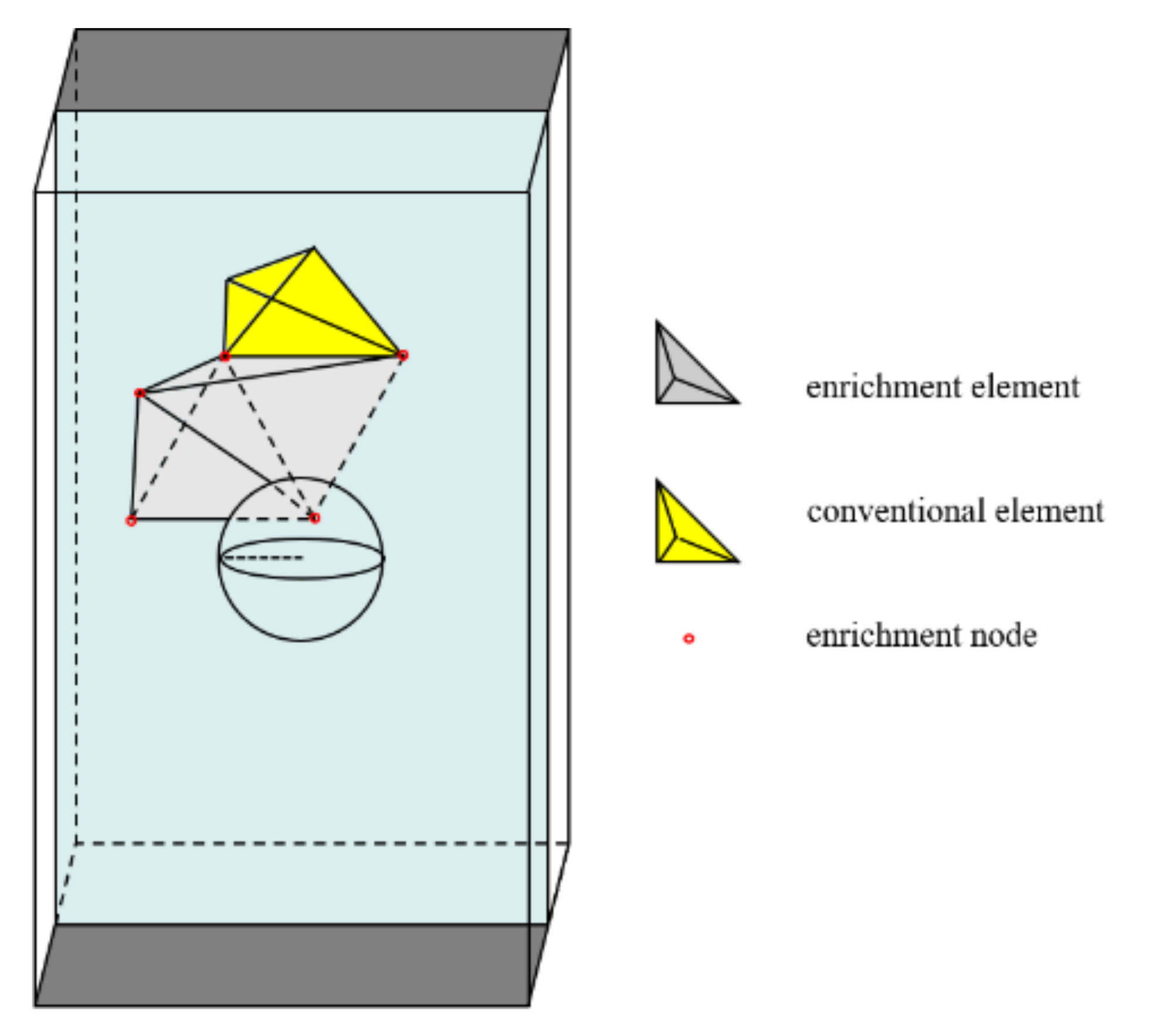
Two or more materials may be found in one element in XFEM. These elements crossed by the interface are so-called enrichment elements. Figure 1 shows the enrichment element and the conventional finite element in the 3D tetrahedron element.

The level set method can be used to locate an interface or even track its movement. A spatially high one-dimensional level set function ϕ denotes the interface under study, and the zero level set denotes the location of the interface. For the 3D electrostatic field problem studied in this paper, assuming that the bubble is a sphere with the center (x₀, y₀, z₀), the level set function ϕ can be chosen as:

$$\varphi (x,y,z)={(x-x_0)}^2+{(y-y_0)}^2+{(z-z_0)}^2-r^2$$

(1)

where x, y, z are the coordinates of a point; r is the radius of the sphere.

Figure 2 is the schematic diagram of the 4D level set function. Different colors represent different function values. There are the same function value and color on the surface of the bubble sphere.

This paper takes the improved XFEM method in the electrostatic field as an example. An improved XFEM is presented to solve the Poisson equation shown in Equation (2) for fast calculation of 3D potential distribution.

$$\nabla \cdot (\epsilon \nabla \phi )=-\frac{\rho }{{\epsilon }_0}$$

(2)

where φ is the potential, ε represents the permittivity of the medium, ε₀ represents the vacuum permittivity, and ρ stands for bulk charge density.

Equation (3) shows the interpolation function of potential used by CFEM. XFEM improves the approximate solution expression of CFEM. The material interface is taken into account and a set of degrees of freedom of enrichment nodes is added. XFEM interpolation function is shown in Equation (4).

$$\phi (x,y,z)={\displaystyle \sum _{i\in I}{N}_i(x,y,z){\alpha }_i}$$

(3)

$$\phi (x,y,z)={\displaystyle \sum _{i\in I}{N}_i(x,y,z){\alpha }_i}+{\displaystyle \sum _{j\in I^{*}}{N}_j(x,y,z)\Phi (x,y,z){\beta }_j}$$

(4)

$$\Phi (x,y,z)={\displaystyle \sum _I{N}_i(x,y,z)\cdot \left|{\varphi }_i\right|}-\left|{\displaystyle \sum _I{N}_i(x,y,z)}\cdot {\varphi }_i\right|$$

(5)

in the discretized domain, where I is the set of all nodes, I* is the set of the enriched nodes, I*∈I, N_i, N_j are the shape functions, Φ is the enrichment function as shown in Equation (5), and α_i and β_j are nodal unknowns.

Much electrical equipment has a complex structure and contains a large number of dense thin layers. The space size of different parts sometimes differs by dozens or even thousands of orders of magnitude. The improved XFEM adjusts the description method of interfaces. By setting a corresponding level set function for each interface, it allows more than two interfaces to appear in one element. The level set on each node is no longer a single value but multiple values due to the number of interfaces in the element.

The interface description method when there are two interfaces in the same element under 3D XFEM is shown in Figure 3. The level set function value increases gradually from the center of the sphere to the outside. The value of the function at the interface is zero. The approximate expression of improved XFEM potential is shown as follow:

$$\phi (x,y,z)={\displaystyle \sum _{i\in I}{N}_i(x,y,z){\alpha }_i}+{\displaystyle \sum _k^N{\displaystyle \sum _{j\in I^{*}}{N}_j(x,y,z){\Phi }_{(k)}(x,y,z){\beta }_{j(k)}}}$$

(6)

where k = 1, 2, …, N, which is the indexing of the interface.

This improved XFEM using the 4D level set function is proposed based on 1D and quasi 3D improved XFEM methods. The scope of application is 3D electromagnetic field numerical calculation. The formula of the unknowns α_i and β_j can be informed as:

$$\begin{array}{c}\frac{\partial W(\phi )}{\partial {\alpha }_i}=\epsilon {\displaystyle \underset{D}{\iint }(\frac{\partial {\phi }^e}{\partial x}\cdot \frac{\partial (\partial {\phi }^e/\partial x)}{\partial {\alpha }_i}+\frac{\partial {\phi }^e}{\partial y}\cdot \frac{\partial (\partial {\phi }^e/\partial y)}{\partial {\alpha }_i}+\frac{\partial {\phi }^e}{\partial z}\cdot \frac{\partial (\partial {\phi }^e/\partial z)}{\partial {\alpha }_i})\mathrm{d}x\mathrm{d}y\mathrm{d}z}\\ \frac{\partial W(\phi )}{\partial {\beta }_i}=\epsilon {\displaystyle \underset{D}{\iint }(\frac{\partial {\phi }^e}{\partial x}\cdot \frac{\partial (\partial {\phi }^e/\partial x)}{\partial {\beta }_j}+\frac{\partial {\phi }^e}{\partial y}\cdot \frac{\partial (\partial {\phi }^e/\partial y)}{\partial {\beta }_j}+\frac{\partial {\phi }^e}{\partial z}\cdot \frac{\partial (\partial {\phi }^e/\partial z)}{\partial {\beta }_j})\mathrm{d}x\mathrm{d}y\mathrm{d}z}\end{array}$$

(7)

3. Numerical Examples

Numerical models are established to verify the reliability of the 3D improved XFEM. Different materials may be found in one element under improved XFEM. This characteristic makes it possible to omit the step of repartition of mesh while the bubble rises and deforms.

According to [11,12,13,14,15], under the action of a uniform electric field at MV/m level, bubbles are gradually stretched and lengthened as they rise, from spheres to ellipsoids. To verify the accuracy of improved XFEM, numerical examples are designed imitating the experiments in the literature.

In Section 3.1 and Section 3.2, the potential distribution in liquid nitrogen is analyzed without considering the bubble movement and deformation. In these two parts, bubbles are considered to be fixed. Only the electric field at a certain moment is analyzed. Referring to [11,14], the radius of bubbles is around 1.5 mm. The center position and radius of multiple bubbles are generated randomly in the solution domain.

In Section 3.3, the motion of a bubble under an electric field in liquid nitrogen is calculated. The movement and deformation process are calculated through the commercial software COMSOL Multiphysics 5.1 provided by COMSOL AB from Stockholm, Sweden. The position of the gas–liquid interface is applied to the XFEM calculation as a known condition.

3.1. Single Bubble

The bubble exists between two parallel plate electrodes; it is equivalent to a sphere. The uniform electric field intensity is about 2 MV/m. The potential on the upper plate is 50,000 V, and the lower plate is grounded. The uniform electric field intensity is about 2 MV/m. The boundary condition of the side walls is shown as Equation (8). The 3D sketch is shown in Figure 4.

$$\epsilon \frac{\partial \phi }{\partial n}=0$$

(8)

where n represents the unit normal vector at the interface.

Figure 5 shows the mesh grid of CFEM. The whole solution domain is a 15 mm × 15 mm × 25 mm hexahedron. There is a sphere representing the bubble in the center of the hexahedron. Its radius is assumed to be 1.5 mm. The relative permittivity of liquid nitrogen is 1.4 and that of gas is 1.

Table 1. Contrast of number of nodes and elements.

Method	Node Number	Element Number	Calculation Time
CFEM	1400	7062	57 s
XFEM	1159	5626	37 s

compares the number of nodes and elements generated by two methods. CFEM needs to consider the interface of different materials. Improved XFEM can eliminate this process, simplifying the mesh. The number of nodes and elements is reduced, which makes the calculation process faster.

Calculate the potential distribution of the single-bubble model with CFEM and XFEM. A plane parallel to the YOZ plane is made through the center of the bubble sphere. Draw a potential distribution cloud on this section. The potential sectional at x = 7.5 mm of XFEM is shown in Figure 6. It can be seen that the electric field around the bubble is distorted, which is consistent with the actual situation and the CFEM calculation results.

The comparison results of electric potential at the same coordinate position show that the XFEM method has high accuracy. The average relative error of 1159 nodes is 0.39% and the maximum relative error is 7.79%.

The electric field of the node near the interface changes rapidly. Around the surface of the sphere, select the 10 nodes closest to the sphere to compare the calculation results, shown in

Table 2. Contrast of the results of nodes near interface.

Nodes	CFEM	XFEM	Relative Error
1	24,986.10	25,011.4	0.10%
2	25,262.10	25,304.2	0.17%
3	24,638.90	24,704.4	0.27%
4	24,680.60	24,704.7	0.10%
5	25,268.40	25,343.1	0.30%
6	24,596.60	24,646.4	0.20%
7	23,587.80	24,521.7	3.96%
8	24,887.50	24,959.3	0.29%
9	24,987.70	25,010.3	0.09%
10	19,976.10	18,419.6	−7.79%

.

3.2. Multi-Bubbles

Multi-bubble models are built to illustrate the superiority of XFEM in dealing with more media interface problems. In these two examples, the interaction and coalescence among bubbles are ignored. The boundary conditions are the same as the single-bubble model.

3.2.1. 5 Bubbles

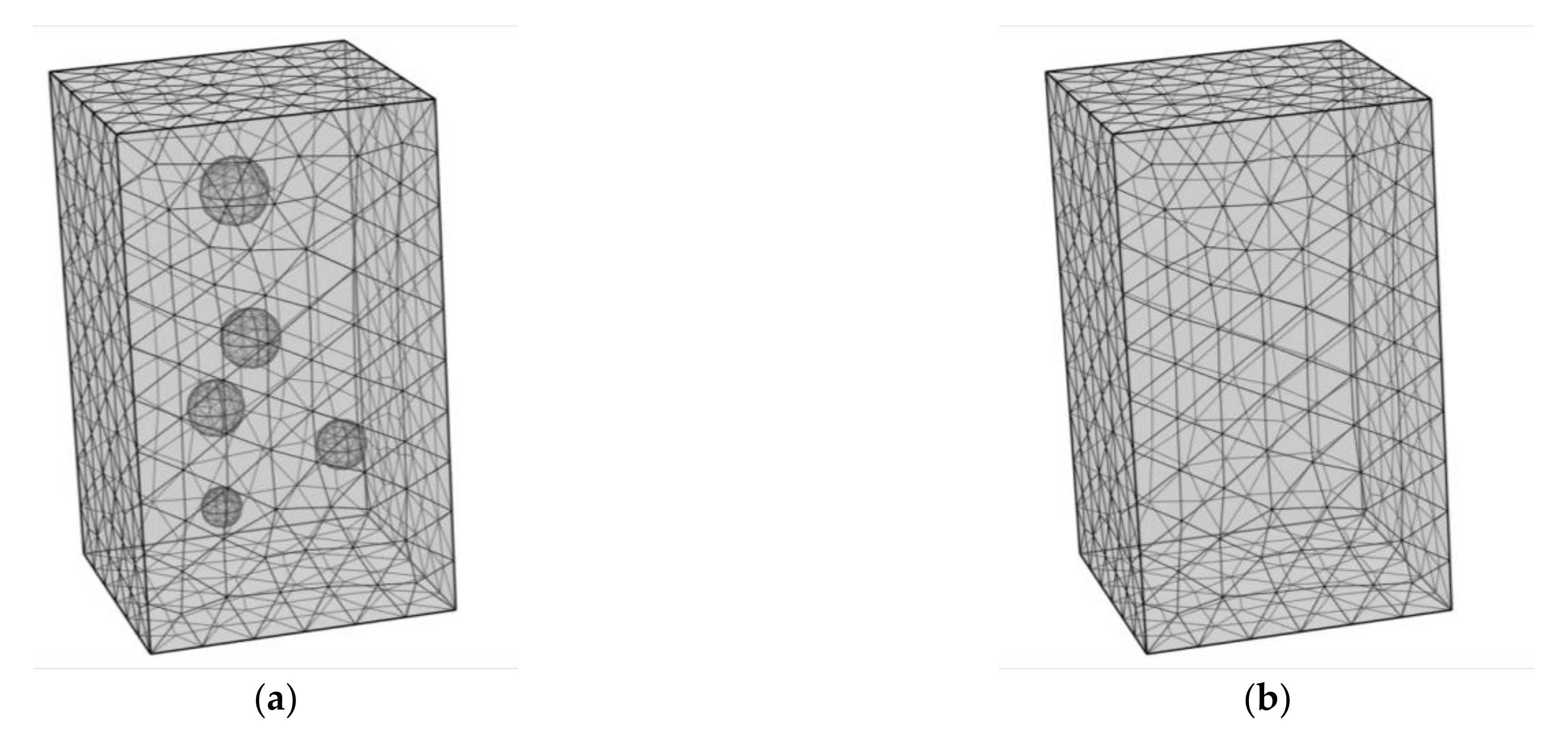
The whole solution domain is a 15 mm × 15 mm × 25 mm hexahedron. There are 5 bubbles set in the hexahedron. Figure 7 shows 3D mesh grid of 5 bubbles.

Table 3. The center position and radius of 5 bubbles.

Number	Center Position	Radius (mm)
Bubble 1	(7.5, 7.5, 12.5)	1.50
Bubble 2	(2, 3, 5)	1.30
Bubble 3	(8, 8, 20)	1.70
Bubble 4	(10, 10, 5)	1.00
Bubble 5	(10, 10, 10)	1.40

shows the coordinates of each spherical and radius.

Compared with the CFEM, improved XFEM greatly simplifies the mesh.

Table 4. Contrast of number of nodes and elements in 5 bubbles.

Method	Node Number	Element Number	Calculation Time
CFEM	2407	12,997	4 min 43 s
XFEM	1159	5626	34 s

compares the number of nodes and elements generated by two methods, as well as the calculation time cost on the same computer. Select the section with dense bubbles to draw the potential map. The potential sectional at y = 10 mm and x = 7.5 mm of XFEM is shown in Figure 8.

Among the 1159 nodes, the maximum relative error is 7.93% and the average relative error is 1.04%. Ten nodes near the boundary of the sphere are selected to compare the calculation results. The comparison is shown in

Table 5. Contrast of the results of nodes near interface.

Nodes	CFEM	XFEM	Relative Error
1	25,529.1	24,719.4	−3.17%
2	26,045.3	25,304.1	−2.85%
3	24,368.2	24,691.6	1.33%
4	24,836.3	24,988.6	0.61%
5	24,609.9	25,023.2	1.68%
6	24,554	24,954	1.63%
7	23,440.8	25,300.7	7.93%
8	24,708.2	25,028	1.29%
9	24,411.8	24,645.7	0.96%
10	24,316.5	24,635.1	1.31%

.

3.2.2. 10 Bubbles

Figure 9 shows a 3D multi-bubbles mesh grid.

Table 6. The center position and radius of 10 bubbles.

Number	Center Position	Radius (mm)
Bubble 1	(7.5, 7.5, 12.5)	1.50
Bubble 2	(2, 3, 5)	1.30
Bubble 3	(8, 8, 20)	1.70
Bubble 4	(10, 10, 5)	1.00
Bubble 5	(10, 10, 10)	1.40
Bubble 6	(12.5, 2.5, 7.5)	1.40
Bubble 7	(8, 4, 2)	1.20
Bubble 8	(5, 11, 14)	1.70
Bubble 9	(4, 5, 16)	1.50
Bubble 10	(3, 9, 8)	1.40

shows the coordinates of each spherical and radius. The number of nodes and elements generated by two methods, as well as the calculation time cost on the same computer, are compared in

Table 7. Contrast of number of nodes and elements.

Method	Node Number	Element Number	Calculation Time
CFEM	3582	19,851	15 min 47 s
XFEM	1159	5626	34 s

. Select the section with dense bubbles to draw the potential map. The potential sectional at y = 10 mm and x = 7.5 mm of XFEM is shown in Figure 10.

Among the 1159 nodes, the maximum relative error is 7.93% and the average relative error is 2.52%. Ten nodes near the boundary of the sphere are selected to compare the calculation results. The comparison is shown in

Table 8. Contrast of the results of nodes near interface.

Nodes	CFEM	XFEM	Relative Error
1	20,288	19,907.7	−1.87%
2	22,955	24,775.6	7.93%
3	46,363	46,548.6	0.40%
4	35,053	35,484.3	1.23%
5	28,163	28,853.9	2.45%
6	38,021	38,472.6	1.19%
7	7426.6	7017.14	−5.51%
8	12,749	12,978.8	1.80%
9	3042.8	2818.45	−7.37%
10	20,027	20,461.1	2.17%

.

Section 3.1 and Section 3.2 show that the improved XFEM can save calculation costs and reduce calculation time compared with CFEM. At the same time, the accuracy of XFEM calculation results rises with the increase of model complexity. The calculation saved and the contrast of accuracy are shown in

Table 9. Contrast of calculation saving and accuracy.

Method	Single Bubble		5 Bubbles		10 Bubbles
	Elements	Calculation Time	Elements	Calculation Time	Elements	Calculation Time
CFEM	7062	57 s	12,997	4 min 51 s	19,851	15 min 47 s
XFEM	5626	37 s	5626	34 s	5626	34 s
Ratio	79.66%	64.91%	53.28%	11.68%	28.34%	3.6%

.

As the complexity of the model increases, the ratio of element saving and time-saving increases. The calculation accuracy decreases. The average relative error of the single-bubble model is 0.39%, while the average relative error of the 10-bubble model increases to 2.52%.

3.3. Moving-Deformed Bubble

The rising process of a bubble between electrodes in liquid nitrogen is calculated by COMSOL Multiphysics 5.1 provided by COMSOL AB. Under the action of buoyancy and electromagnetic force, the bubble gradually floats up and changes into an ellipsoid. Its volume will change during this process figure [16,17,18].

The trajectory of the bubble in liquid nitrogen is calculated in COMSOL Multiphysics 5.1 with the Fluid Flow and Electrostatics modules. As shown in Figure 11, the entire solution domain is 10 mm × 10 mm × 10 mm. There is a 1.5 mm radius bubble in the center. The liquid material is liquid nitrogen and the bubble material is nitrogen. The temperature is 77 K. The upper and lower plates are set to No Flow, with 20,000 V voltage added to the top and grounded to the bottom. The initial liquid flow rate is 0. Add gravity along the Z direction. The movement and deformation of the bubble at different times are shown in Figure 12.

The coordinates of the points on the gas–liquid interface at different times calculated by the software are exported. According to the position of the gas–liquid interface at different times, the electric field calculation model is established, and the potential distribution is calculated by CFEM and improved XFEM, respectively.

Figure 13 shows mesh grids for three different times in CFEM and one mesh grid for improved XFEM.

CFEM is limited by its characteristics. With the change of bubble shape and position, the mesh generation process is repeated at different times. XFEM is an excellent meshless computing method, which can omit the steps of repeated meshing. The same mesh grid can be used in different states, greatly reducing the calculation time cost.

The comparison of node number and elements number of the model under CFEM and XFEM is shown in

Table 10. Contrast of number of nodes and elements.

Method	Node Number	Element Number
CFEM 0 s	3218	16,876
CFEM 0.025 s	3214	16,818
CFEM 0.035 s	3328	17,516
Total of CFEM	9760	51,210
XFEM	3167	16,553

. CFEM meshed three times in three moments, while XFEM only meshed once.

Figure 14 shows the potential distribution on slices parallel to the XZ plane through the center of the sphere. In a total of 3167 nodes, the potential calculation results at 3 moments are compared. The comparison results are shown in

Table 11. Contrast of calculation results.

Time	Maximum Relative Error (%)	Average Relative Error (%)
0 s	−8.65%	1.6%
0.025 s	−4.05%	1.06%
0.035 s	−3.59%	1.14%
Total	−8.65%	1.27%

.

4. Conclusions

Three kinds of bubble models in liquid nitrogen were established and calculated by CFEM and XFEM, respectively. By comparing the number of nodes, the number of elements, and the calculation results of the two methods, it is shown that XFEM can reduce the number of nodes and elements required for numerical calculation and reduce the calculation consumption. At the same time, the results of XFEM are reliable. The ratio of element saving and time saving increases as the complexity of the model increases. But the calculation accuracy decreases. The average relative error of the single bubble model is 0.39%, while the average relative error of the 10-bubble model increases to 2.52%.

Currently, improved XFEM can reduce computational costs by simplifying the mesh grid. XFEM can ignore the effect of interfaces when generating mesh. It has a great advantage when dealing with the calculation of electromagnetic fields in the tip structure and dense interfaces.

However, as the number of elements decreases, some loss of accuracy is unavoidable for XFEM. The accuracy of the discontinuous difference function used by XFEM can be further improved. At the same time, the identification of enrichment elements and the numerical integration in the enrichment elements are important factors that restrict the accuracy of XFEM calculation results. Further optimization and research in these areas are still needed in the future.

References

- Fink, S.; Kim, H.-R.; Mueller, R.; Noe, M.; Zwecker, V. AC breakdown voltage of liquid nitrogen depending on gas bubbles and pressure. In Proceedings of the 2014 ICHVE International Conference on High Voltage Engineering and Application, Poznan, Poland, 8–11 September 2014; pp. 1–4. [Google Scholar]
- Fink, S.; Zwecker, V. Flashover voltage of PE300 insulators embedded in liquid nitrogen with and without gas bubbles. In Proceedings of the IEEE International Conference on Dielectrics (ICD), Montpellier, France, 3–7 July 2016; pp. 1040–1043. [Google Scholar]
- Baek, S.-M.; Kim, H.-J. Shape and dielectric strength of thermal bubbles in liquid nitrogen. J. Korean Inst. Electr. Electron. Mater. Eng. 2015, 25, 326–331. [Google Scholar]
- Lenardo, B.; Li, Y.; Manalaysay, A.; Morad, J.; Payne, C.; Stephenson, S.; Szydagis, M.; Tripathi, M. Position reconstruction of bubble formation in liquid nitrogen using piezoelectric sensors. J. Instrum. 2016, 11, 1–9. [Google Scholar] [CrossRef][Green Version]
- Belytschko, T.; Black, T. Elastic crack growth in finite elements with minimal remeshing. Int. J. Numer. Methods Eng. 1999, 45, 601–620. [Google Scholar] [CrossRef]
- Belytschko, T.; Moës, N.; Usui, S.; Parimi, C. Arbitrary discontinuities in finite elements. Int. J. Numer. Methods Eng. 2001, 50, 993–1013. [Google Scholar] [CrossRef]
- Duan, N.; Xu, W.; Wang, S.; Zhu, J.; Guo, Y. An improved XFEM with multiple high-order enrichment functions and low-order meshing elements for field analysis of electromagnetic devices with multiple nearby geometrical interfaces. IEEE Trans. Magn. 2015, 51, 7206004. [Google Scholar]
- Duan, N.; Xu, W.; Wang, S.; Zhu, J. Current Distribution Calculation of Superconducting Layer in HTS Cable Considering Magnetic Hysteresis by Using XFEM. IEEE Trans. Magn. 2018, 54, 8000804. [Google Scholar] [CrossRef]
- Duan, N.; Xu, W.; Wang, S.; Zhu, J. Quasi-3-D Cylindrical Coordinate XFEM Model of HTS Cable. IEEE Trans. Magn. 2019, 55, 1–4. [Google Scholar] [CrossRef]
- Duan, N.N.; Xu, W.J.; Wang, S.H.; Li, H.L.; Guo, Y.G.; Zhu, J.G. Extended finite element method for electromagnetic fields. In Proceedings of the 2015 IEEE International Conference on Applied Superconductivity and Electromagnetic Devices (ASEMD), Shanghai, China, 20–23 November 2015; pp. 364–365. [Google Scholar]
- Dong, W.; Li, R.; Yu, H.; Yan, Y. An investigation of behaviours of a single bubble in a uniform electric field. Exp. Therm. Fluid Sci. 2005, 30, 579–586. [Google Scholar] [CrossRef]
- Wang, P.; Swaffield, D.; Lewin, P.; Chen, G. The effect of an electric field on behaviour of thermally induced bubble in liquid nitrogen. In Proceedings of the IEEE International Conference on Dielectric Liquids, Poitiers, France, 30 June–3 July 2008; pp. 1–4. [Google Scholar]
- Medvedev, D.A.; Kupershtokh, A.L.; Bukovets, A.A. Bukovets, Dynamics of bubble in dielectric liquid in electric field: Mesoscopic simulation. In Proceedings of the 2017 IEEE 19th International Conference on Dielectric Liquids (ICDL), Manchester, UK, 25–29 June 2017; pp. 1–4. [Google Scholar]
- Korobeynikov, S.M.; Karpov, D.I.; Ridel, A.V.; Ovsyannikov, A.G.; Meredova, M.B.; Kupershtokh, A.L. Experimental study and numerical simulation of partial discharges in deformed bubbles in transformer oil. In Proceedings of the 2019 IEEE 20th International Conference on Dielectric Liquids (ICDL), Rome, Italy, 23–27 June 2019; pp. 1–4. [Google Scholar]
- Kupershtokh, A.L.; Medvedev, D.A. Dynamics of bubbles in liquid dielectrics under the action of an electric field: Lattice Boltzmann method. In Proceedings of the 4th All-Russian Scientific Conference Thermophysics and Physical Hydrodynamics with the School for Young Scientists, Yalta, Crimea, 15–22 September 2019. [Google Scholar]
- Albadawi, A.; Donoghue, D.; Robinson, A.; Murray, D.; Delauré, Y. Influence of surface tension implementation in the volume of fluid and coupled volume of fluid with level set methods for bubble growth and detachment. Int. J. Multiph. Flow 2013, 53, 11–28. [Google Scholar] [CrossRef]
- Yamamoto, T.; Okano, Y.; Dost, S. Validation of the S-CLSVOF method with the density-scaled balanced continuum surface force model in multiphase systems coupled with thermocapillary flows. Int. J. Numer. Method Fluids 2017, 83, 223–244. [Google Scholar] [CrossRef]
- Taqieddin, A.; Liu, Y.; Alshawabkeh, A.N.; Allshouse, M.R. Computational Modeling of Bubbles Growth Using the Coupled Level Set—Volume of Fluid Method. Fluids 2020, 5, 120. [Google Scholar] [CrossRef]
Figure 1.
Enrichment elements in 3D tetrahedron elements.
Figure 2.
4D level set function.
Figure 3.
(a) The level set function of the first interface; (b) The level set function of the second interface.
Figure 4.
3D single bubble model in liquid nitrogen.
Figure 5.
(a) 3D single bubble mesh grid of CFEM; (b) 3D single bubble mesh grid of XFEM.
Figure 6.
Single bubble potential distribution at x = 7.5 mm.
Figure 7.
(a) 3D 5 bubbles mesh grid of CFEM; (b) 3D 5 bubbles mesh grid of XFEM.
Figure 8.
(a) 5 bubbles potential diagram at y = 10 mm; (b) 5 bubbles potential diagram at x = 7.5 mm.
Figure 9.
(a) 3D 10 bubbles mesh grid of CFEM; (b) 3D 10 bubbles mesh grid of XFEM.
Figure 10.
(a) 10 bubbles potential diagram at y = 10 mm; (b) 10 bubbles potential diagram at x = 7.5 mm.
Figure 11.
Numerical simulation model of bubble rising in liquid nitrogen.
Figure 12.
(a) Bubble at 0 s; (b) Bubble at 0.025 s; (c) Bubble at 0.035 s.
Figure 13.
(a) Mesh grid of CFEM at 0 s; (b) Mesh grid of CFEM at 0.025 s; (c) Mesh grid of CFEM at 0.035 s; (d) Mesh grid of XFEM for all times.
Figure 14.
(a) Potential distribution on the cross section at 0 s; (b) Potential distribution on the cross section at 0.025 s; (c) Potential distribution on the cross section at 0.035 s.