Transmission Phase Control of Annular Array Transducers for Efficient Second Harmonic Generation in the Presence of a Stress-Free Boundary

Abstract

The through-transmission (TT) method is mainly used to measure the amplitude of the second harmonic from which the acoustic nonlinear parameter is determined for early damage detection of materials. The pulse echo (PE) method, however, has been excluded from nonlinear studies of solid materials because the stress-free boundary suppresses the generation of second harmonics. It is more demanding to develop the PE method for practical applications and this paper considers a novel phase shift technique of annular array transducers to improve second harmonic generation (SHG) at the stress-free boundary. The fundamental and second harmonic fields after phase-shifted radiation are calculated, and their received amplitudes are investigated. The phase difference between the two second harmonic components after reflection from the stress-free boundary is analyzed to explain the enhanced SHG. The PE method with optimal phase shift can generate an improved second harmonic amplitude as high as about 45% of the TT method. Four element array transducers are also found to be more efficient in improved SHG than two element transducers.

1. Introduction

Ultrasonic nondestructive evaluation allows the detection of defects within a material or structure. This plays an important role in preventing failures and is especially important in inspecting load-bearing components used in the industry [1]. So-called micro-defects or damage, such as internal stress, closed cracking, and zero-volume delamination, are generally the forerunners of material cracking and subsequent failures. Microscopic changes due to precipitation, dislocation and embrittlement affect the overall properties of the material. However, measurements of conventional linear ultrasonic parameters, such as sound velocity, attenuation, and backscattering, are not sensitive to these inhomogeneities and do not provide quantitative information on material condition [2]. Nonlinear acoustic methods, such as second harmonic generation (SHG) and measurement of acoustical nonlinear parameters, have proven useful for detecting these types of material defects [3,4,5].

When finite amplitude ultrasonic waves propagate in a material, the nonlinear elastic properties of the material distort the waveform and generate harmonics [6]. Nonlinear ultrasound methods often measure the second harmonic generation (SHG) to obtain a nonlinear parameter β, defined as the ratio of the second harmonic amplitude to the square of the fundamental wave amplitude, and draw conclusions about the material state. Nonlinear parameters can be measured, using longitudinal waves [7,8,9,10,11], Rayleigh waves [12,13,14], and Lamb waves [15,16,17]. Rayleigh waves require sufficient propagation distance to measure SHG; the measured nonlinearity is averaged over distance and cannot be localized. In addition, it is sometimes difficult to obtain pure, nonlinear Rayleigh waves because a certain setup can introduce source nonlinearity. Lamb waves have limited use because they propagate in very thin plates and there are few modes that meet the requirement for cumulative propagation. In contrast, longitudinal waves have been widely used for nonlinear characterization of materials. However, experiments are usually performed in the through-transmission (TT) mode requiring access to both sides, and this technique may be limited in field applications where access is only possible on the external surface of the component.

A practical method for nonlinear ultrasonic measurements, using the normal incidence of longitudinal waves is pulse-echo (PE) testing, which uses only one side of the specimen. Biomedical imaging [18,19] and fluid nonlinearity [20,21] were studied in the PE mode, using heavy metals as reflectors to resemble the rigid boundary condition. However, the problem of PE nonlinear testing of solids with stress-free surfaces is that such boundaries suppress the SHG process and make it hard to acquire reliable nonlinear parameters. In the case of pure plane waves, the harmonic component generated during forward propagation is reflected off the stress-free boundary and decreases to zero after returning to the initial position [22,23]. This is because the two second harmonic components—the reflected and newly generated second harmonics—cancel each other out due to their phase difference of $\pi$ after being reflected from the stress-free boundary. According to theory and experiment, however, the received second harmonic amplitude reflected from the stress-free boundary is not really zero due to the finite size transducer and material attenuation. The currently available pulse-echo nonlinear testing method basically requires the test sample to be thick enough and may not be accurate for thin samples in nonlinear parameter measurements [24,25].

An acoustic beam focused on a stress-free boundary was proven to improve SHG during back propagation from the stress-free boundary [26]. A recent study showed that the phase difference is about $\pi /2$ between the two second harmonic components when a focused beam is used in water [27]. Thus, the received second harmonic amplitude is greatly increased due to the constructive interference of these two components and can be measured in the pulse-echo mode. This study was conducted in fluids where a focused beam can easily be formed. Phased array transducers can produce focused beams in flat solid samples, but it is not easy to create a tightly focused beam, especially with a small number of elements. Therefore, we need to devise another way to create nonlinear beam fields that can produce a phase difference of about $\pi /2$ in the presence of the stress-free boundary. A dual element transducer with a phase shift of the input signal in one element relative to the other was found to improve the SHG in the pulse-echo test simulation of thick samples [28]. A multiple element transducer can provide more options in the control of phase shifts and improve SHG in the pulse-echo setup of thin solid samples.

This paper investigates the efficient SHG from the stress-free boundary of a nonlinear solid by control of the transmission phase shift of array elements. When a sound beam radiates from annular array elements with different phase shifts, the fundamental and second harmonic waves, which are reflected from the rigid or stress-free boundary, are calculated in the pulse-echo setup and their characteristic behavior are examined based on the magnitude of received amplitudes. The phase difference between the reflected and newly generated second harmonic components is completely analyzed to explain the enhanced SHG in solid samples. We also study the effects of various phase shifts applied to array transducers. Simulation results are also given for the case of the plane wave and a single element transducer to check the diffraction effects and the through-transmission results. Optimal phase shifts for a given sample thickness and frequency are illustrated in terms of SHG and nonlinear parameter determination.

2. Theory

Consider nonlinear wave fields reflected from a planar stress-free boundary, as shown in Figure 1, where a pulse-echo testing setup is schematically displayed. In the forward propagation direction of Figure 1, $v_{1i}$ is the particle velocity of the fundamental wave and $v_{2i}$ is the generated second harmonic due to the forcing of $v_{2i}$. In the backward propagation direction, $v_{1r}$ represents the boundary-reflected wave of $v_{1i}$. As discussed in our previous study [21], the nonlinear wave after reflection consists of two components, $v_{2r1}$ and $v_{2r2}$, where $v_{2r1}$ is the second harmonic generated by the reflected $v_{1r}$ and $v_{2r2}$ is the reflected second harmonic when $v_{2i}$ hits the boundary. The total second harmonic after reflection, $v_{2r}$, is then obtained by adding $v_{2r1}$ and $v_{2r2}$. The stress-free boundary is located at $z=z_0$. The acoustic impedance of the solid sample (medium 1) is $z_1={\rho }_1{c}_1$ and the acoustic impedance of medium 2 (air) is $z_2={\rho }_2{c}_2\approx 0$. Therefore, the reflection coefficient of the fundamental and the second harmonic is assumed to be $R_1=R_2\approx -1$.

Nonlinear wave equations are needed to study wave propagation, reflection and SHG in nonlinear solids. For this purpose, the Westervelt equation or the KZK (Khokhlov–Zabolotskaya–Kuznetsov) equation is a suitable model equation because they can account for the effects of nonlinearity, diffraction and attenuation [6]. Compared to the KZK equation, the Westervelt equation is described by three-dimensional coordinates and the solution of the quasilinear equation is valid for all axial ranges. These equations were used to model the nonlinear wave fields in fluids, but they are also suitable for use in solid materials when longitudinal waves are employed exclusively. In this work, we introduce the Westervelt-like equation for calculating the longitudinal wave fields in nonlinear solids.

Several types of planar transducers are considered in this study, as shown in Figure 2. Figure 2a is a single element transducer that will be used for comparison purposes. Since this transducer has only one element, it works both as a transmitter and as a receiver. The annular array transducer of Figure 2b has four concentric elements of equal width [29]. This transducer will be used to apply the transmission phase shift to each element to improve SHG at the stress-free boundary. The emitted waves from the transducer elements will have different phases. The phase shift of each element can be controlled independently. Compared to a two-element transducer, a four-element transducer allows finer phase shifting and is, therefore, much more effective for SHG.

A dual element transducer with phase-shifted radiation (Figure 2c) was shown to be useful in generating improved SHG in pulse-echo testing of thick samples [28] and will be used here for comparison purposes. We will also consider a focused beam using the four-element array transducer of Figure 2b and compare the received wave fields with the phase-shifted radiation. The array beam will be focused on the reflecting boundary by applying appropriate time delays to each element [30].

2.1. Pure Plane Wave

As can be seen in Figure 2a, if the size of the transducer is large enough, the propagation wave can be treated as a plane wave. When the nonlinear parameter β is introduced for a solid medium, the one-dimensional longitudinal wave equation can be expressed as follows [9]:

$$\frac{{\partial }^{2}u}{\partial t^2}=c^2\frac{{\partial }^{2}u}{\partial z^2}\left(1+\beta \frac{\partial u}{\partial z}\right)$$

(1)

where u is the wave particle displacement, t is the time, c is the wave velocity, and z is the one-dimensional coordinate. In Equation (1), $\beta$ is the nonlinear parameter of solids and defined as $\beta =-(3+C_{111}/C_{11})$ where $C_{11}$ and $C_{111}$ are the second- and third-order elastic constants.

Using a standard perturbation theory yields the quasilinear system of equations for the fundamental and second harmonic displacements $u_1$ and $u_2$, respectively. The solutions are then obtained as follows:

$$u=U\sin \left(kz-\omega t\right)+\frac{\beta U^2{k}^{2}z}{8}\cos 2\left(kz-\omega t\right)$$

(2)

where U is the uniform source displacement at the transmitter surface, $k=\omega /c$ is the wave number and $\omega$ is the angular frequency. If the amplitudes of the fundamental and second harmonic are represented as $A_1=U$ and $A_2=\beta U^2{k}^{2}z/8$, the nonlinear parameter $\beta$ can be obtained as follows:

$$\beta =\frac{8A_2}{k^{2}z{A}_1^2}$$

(3)

When the fundamental wave encounters the boundary in the propagation path, it will reflect with its amplitude determined by the reflection coefficient. In the case of the second harmonic wave, as stated previously in Figure 1, two second harmonic components will reflect from the boundary and propagate back to the initial source position [19]. The stationary phase method can be used [20] to write the reflected wave fields in terms of the initial sound source and the coordinate system. Thus, the reflected fundamental and second harmonic waves propagating in the backward direction can be expressed as follows:

$$u_{1r}=R_1\times U\sin \left(kz-\omega t\right)$$

(4)

$$\begin{array}{cc}\hfill u_{2r}& =u_{2r1}+u_{2r2}\hfill \\ & =R_2\times \left(\frac{\beta U^2{k}^2{z}_0}{8}\right)\cos 2\left(kz-\omega t\right)+R_1^2\times \left(\frac{\beta U^2{k}^2(z-z_0)}{8}\right)\cos 2\left(kz-\omega t\right)\hfill \\ & =\frac{\beta U^2{k}^2}{8}\left(R_2{z}_0+R_1^2(z-z_0)\right)\cos 2\left(kz-\omega t\right)\hfill \end{array}$$

(5)

where $z_0$ is the distance between the transmitting plane and the boundary, and $R_1$ and $R_2$ are the reflection coefficients for the fundamental and second harmonics, respectively. In Equation (5), the first term represents the reflected second harmonic and the second term represents the newly generated one. The reflection coefficients of the fundamental and second harmonic waves can be assumed to be $R_1=R_2=-1$ for the stress-free boundary, and $R_1=R_2=1$ for the rigid boundary when the longitudinal wave is incident perpendicular to the boundary.

The nonlinear parameter in the pulse-echo mode can be defined from Equations (4) and (5) as the following:

$$\beta =\frac{8A_2}{k^2{A}_1^2}\left[\frac{R_1^2}{R_2{z}_0+R_1^2(z-z_0)}\right]$$

(6)

where $A_1$ and $A_2$ are the amplitudes of the fundamental and second harmonic waves after being reflected from the boundary. In Equation (6), $\beta$ is not defined at $z=2z_0$ for the stress-free boundary since the total second harmonic amplitude is 0 in this case. In the case of the rigid boundary, the $\beta$ corresponds to that of the through-transmission mode with the sample thickness $2z_0$. It is also noted that any harmonic content generated in the forward path is cancelled by the nominally equal and opposite phase of harmonics generated on the return path, as the reflection coefficient is negative ($R_1=R_2=-1$) at the stress-free boundary.

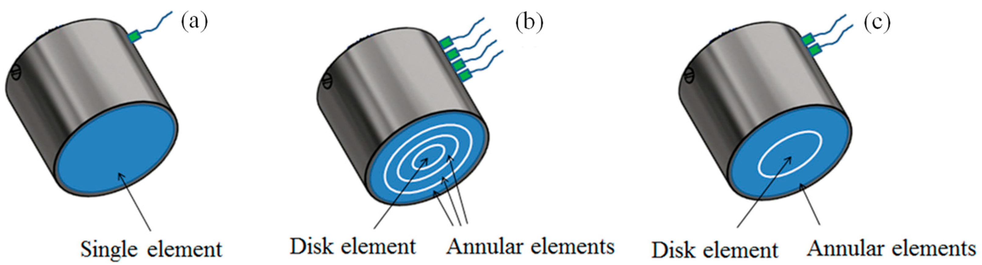
2.2. Single Element Transducer

When a finite-size transducer is used to generate and receive nonlinear waves, the wave diffraction effect should be included in the wave equation. Therefore, we introduce a nonlinear wave equation in the three-dimensional coordinate system to model the propagating and reflecting waves. The attenuation effects will not be considered in this study. In terms of the particle velocity, $v$, the Westervelt-like equation for longitudinal waves can be expressed as follows [15]:

$$\left({\nabla }^2-\frac{1}{c^2}\frac{{\partial }^2}{\partial t^2}\right)v=-\frac{\beta }{c^3}\frac{{\partial }^2{v}^2}{\partial t^2} ,$$

(7)

where the operator ${\nabla }^2$ is the Laplacian in the (x, y, z) space and z is taken as the direction of propagation.

The quasilinear solution is assumed to have the following form:

$$v=v_1\exp (-i\omega t)+v_2\exp (-2i\omega t)$$

(8)

Substitution of Equation (8) into Equation (7) yields the following two equations:

$${\nabla }^2{v}_1+k^2{v}_1=0 ,$$

(9)

$${\nabla }^2{v}_2+4k^2{v}_2=\frac{2\beta k^2}{c}{v}_1^2.$$

(10)

The solutions of the above equations can be obtained by using the Rayleigh integral method and Green’s function approach:

$$v_{1i}(x,y,z)=-2ik{\displaystyle {\int }_S{v}_1(x^{\prime },y^{\prime },0)G_1(x,y,z|x^{\prime },y^{\prime },0)}dS$$

(11)

$$v_{2i}(x,y,z)=\frac{2\beta k^2}{c}{\displaystyle {\int }_0^z{\displaystyle {\int }_{-\infty }^{+\infty }{\displaystyle {\int }_{-\infty }^{+\infty }{v}_{1i}^2(x^{\prime },y^{\prime },z^{\prime })}}} G_2(x,y,z|x^{\prime },y^{\prime },z^{\prime }) d{x}^{\prime }d{y}^{\prime }d{z}^{\prime }$$

(12)

The Green’s function for the nth harmonic is given as follows:

$$G_n(x,y,z|x^{\prime },y^{\prime },z^{\prime })=\frac{1}{4\pi r}\exp (nikr), n=1,2$$

(13)

where $r=\sqrt{{(x-x^{\prime })}^2+{(y-y^{\prime })}^2+{(z-z^{\prime })}^2}$ is the distance from the source point ($x^{\prime },y^{\prime },z^{\prime }$) to the target point ($x,y,z$). The sound source on the transducer surface is defined as the following:

$$\{\begin{array}{l}{v}_1(x^{\prime },y^{\prime },z^{\prime }=0)=v_0(x^{\prime },y^{\prime }), 0\le {x^{\prime }}^2+{y^{\prime }}^2\le a^2\hfill \\ v_2(x^{\prime },y^{\prime },z^{\prime }=0)=0\hfill \end{array}$$

(14)

where a is the radius of the circular transmitting element.

The reflected wave fields can be derived from the stationary phase method when a wave is reflected from a large planar interface [17]. Then, the solution in the backward direction can be expressed as follows:

$$v_{1r}(x,y,z)=R\times \left(-2ik\right){\displaystyle {\int }_S{v}_0(x^{\prime },y^{\prime },z=0)G_1(x,y,z|x^{\prime },y^{\prime },0)}dS$$

(15)

$$\begin{array}{cc}\hfill v_{2r}(x,y,z)& =v_{2r1}(x,y,z)+v_{2r2}(x,y,z)\hfill \\ & =R\times \frac{2\beta k^2}{c}{\displaystyle {\int }_0^{z_0}{\displaystyle {\int }_{-\infty }^{+\infty }{\displaystyle {\int }_{-\infty }^{+\infty }{v}_{1i}^2(x^{\prime },y^{\prime },z^{\prime })}}} G_2(x,y,z|x^{\prime },y^{\prime },z^{\prime }) d{x}^{\prime }d{y}^{\prime }d{z}^{\prime }+\hfill \\ & R_{}^2\times \frac{2\beta k^2}{c}{\displaystyle {\int }_{z_0}^z{\displaystyle {\int }_{-\infty }^{+\infty }{\displaystyle {\int }_{-\infty }^{+\infty }{v}_{1i}^2(x^{\prime },y^{\prime },z^{\prime })}}} G_2(x,y,z|x^{\prime },y^{\prime },z^{\prime }) d{x}^{\prime }d{y}^{\prime }d{z}^{\prime }\hfill \end{array}$$

(16)

The average velocity received by the same transducer at $z=2z_0$ can be obtained by the following integral:

$${\tilde{v}}_n(2z_0)=\frac{1}{S}{\displaystyle {\int }_S{v}_{nr}(x,y,2z_0)}dS,n=1,2$$

(17)

where $dS$ is the receiver area.

Now that the received velocities of the fundamental and second harmonics are available, the nonlinear parameter ${\beta }^{\prime }$ in the pulse-echo setup can be defined in terms of displacement. Using the relationship between velocity and displacement, $v_n=-n\omega u_n, n=1,2$, ${\beta }^{\prime }$ in the pulse-echo mode at $z=2z_0$ can be expressed as follows:

$${\beta }^{\prime }=\frac{8{\tilde{u}}_2}{k^2{z}_0{\tilde{u}}_1^2}$$

(18)

where ${\beta }^{\prime }$ denotes the “uncorrected” or “relative” nonlinear parameter.

2.3. Annular Array Transducer with Phase-Shifted Radiation

When the array transducer shown in Figure 2b is used to generate and receive nonlinear waves, each element of the array transducer can be operated individually. In nonlinear ultrasonic testing, a tone burst with many cycles is typically used to drive the element. Here, we introduce a phase shift technique that improves SHG through phase control of the second harmonic components reflected at the stress-free boundary.

Here is a brief description of the phase shift technique. Figure 3 shows a sine wave of two cycles with the zero phase. Waveforms with phase shifts of $\pi /2$ and π are also shown in the same figure. When every element of an array transducer emits waves without a phase shift, the array transducer works as a single-element transducer. However, when there is a phase shift between the elements, the wave fields in some positions will be strongly enhanced.

A time-delayed signal in the time-domain is equivalent to multiplying the frequency domain signal by the phase term, which is linear in frequency and proportional to the delay. The relationship between the phase angle and the delay time is given by $\varphi =\omega \Delta t$. Thus, the fundamental and second harmonic wave fields generated by an array transducer with the phase shift can be calculated in the frequency domain by introducing an exponential term $\exp (i{\varphi }^{(m)})$ to each element m and adding contributions from all elements.

The single element approach can be extended to calculate the radiated and received beam fields of the four-element array transducer in the pulse-echo mode. Nonlinear interaction that may occur between the elements of the array transducer is ignored. The fundamental velocity fields in the forward propagation region ($0\le z\le z_0$) due to the excitation of the jth element, $v_{1i}^{(j)}$, and the generated second harmonic velocity fields, $v_{2i}^{(j)}$, can be expressed in the same forms as Equations (11) and (12), respectively. The sound source prescribed on the jth element is now given by the following:

$$v_1^j(x^{\prime },y^{\prime },z^{\prime }=0)=\{\begin{array}{l}{v}_0{\mathrm{e}}^{\mathrm{i}{\varphi }^{\left(j\right)}}, 0\le {x^{\prime }}^2+{y^{\prime }}^2\le b_j^2, j=1 (\mathrm{central} \mathrm{disk} \mathrm{element}) \hfill \\ v_0{\mathrm{e}}^{\mathrm{i}{\varphi }^{\left(j\right)}},a_j^2\le {x^{\prime }}^2+{y^{\prime }}^2\le b_j^2, j=2,3,4 (\mathrm{outer} \mathrm{ring} \mathrm{element})\hfill \end{array}$$

(19)

where ${\varphi }^{(j)}$ is the transmission phase shift of the $j^{\mathrm{th}}$ element, and a and b denote the inner and outer diameters, respectively. The diameter $b_1$ of the center disk element is equal to the diameter $a_2$, so there is no gap between the two adjacent elements.

The propagated and reflected velocity fields due to the phase-shifted radiation of the $j^{\mathrm{th}}$ element can be found using the integral solutions for the single-element transducer described in the previous section. Next, it is necessary to calculate the received average velocity of the $j^{\mathrm{th}}$ element by summing the contributions from the phase-shifted radiation of all elements of the array transducer. The average velocity received on each element at the source position ($z=2z_0$) can be written as the following:

$${\tilde{v}}_n^{(j)}(2z_0)=\frac{1}{S_{}^{(j)}}{\displaystyle {\int }_{S_{}^{(j)}}\left[{\displaystyle \sum _{m=1}^4{v}_{nr}^{(m->j)}(x,y,2z_0)e^{i{\varphi }^{(m)}}}\right]}d{S}_{}^{(j)},n=1,2$$

(20)

where $S_{}^{(j)}$ is the area of the jth element, and $v_{nr}^{(m->j)}(x,y,2z_0)e^{i{\varphi }^{(m)}}$ is the reflected velocity arriving at the jth element when the phase-shifted mth element is radiated. Finally, the received total velocity of the nth harmonic is given by the following:

$${\tilde{v}}_n^{}(2z_0)={\displaystyle \sum _{j=1}^4{\tilde{v}}_n^{(j)}}(2z_0)$$

(21)

and the uncorrected nonlinear parameter, ${\beta }^{\prime }$, can be calculated by Equation (18).

3. Simulation Results and Discussion

The fundamental and second harmonic wave fields generated by different types of transducers are calculated in this section to obtain the received average fields. In numerical simulations, the propagation medium is chosen as Al6061 with the wave velocity of c = 6430 m/s and the nonlinear parameter of β = 5.5. To investigate the pulse-echo nonlinear behavior in a relatively thin sample, the sample thickness is set to $z_0=15$ mm. The attenuation was ignored in this study. Each transducer element emits a fundamental wave at a frequency of 5 MHz with the source displacement of u₀ = 1 × 10⁻⁹ m.

The radius of the single-element transducer shown in Figure 2a was chosen to be 12.7 mm. For the four-element array transducer shown in Figure 2b, the inner radii of these elements are r₀ = 0 mm, r₂ = 3.175 mm, r₄ = 6.35 mm and r₆ = 9.525 mm, respectively. The outer radii are r₁ = 3.175 mm, r₃ = 6.35 mm, r₅ = 9.525 mm and r₇ = 12.7 mm. It was assumed that there is no gap between the elements of the array transducer.

The dual element transducer shown in Figure 2c is composed of an outer ring element and a central disk element. The inner and outer diameters of the ring element are 6.35 mm and 12.7 mm, respectively. There is no gap between the two elements, so the diameter of the inner element is 6.35 mm.

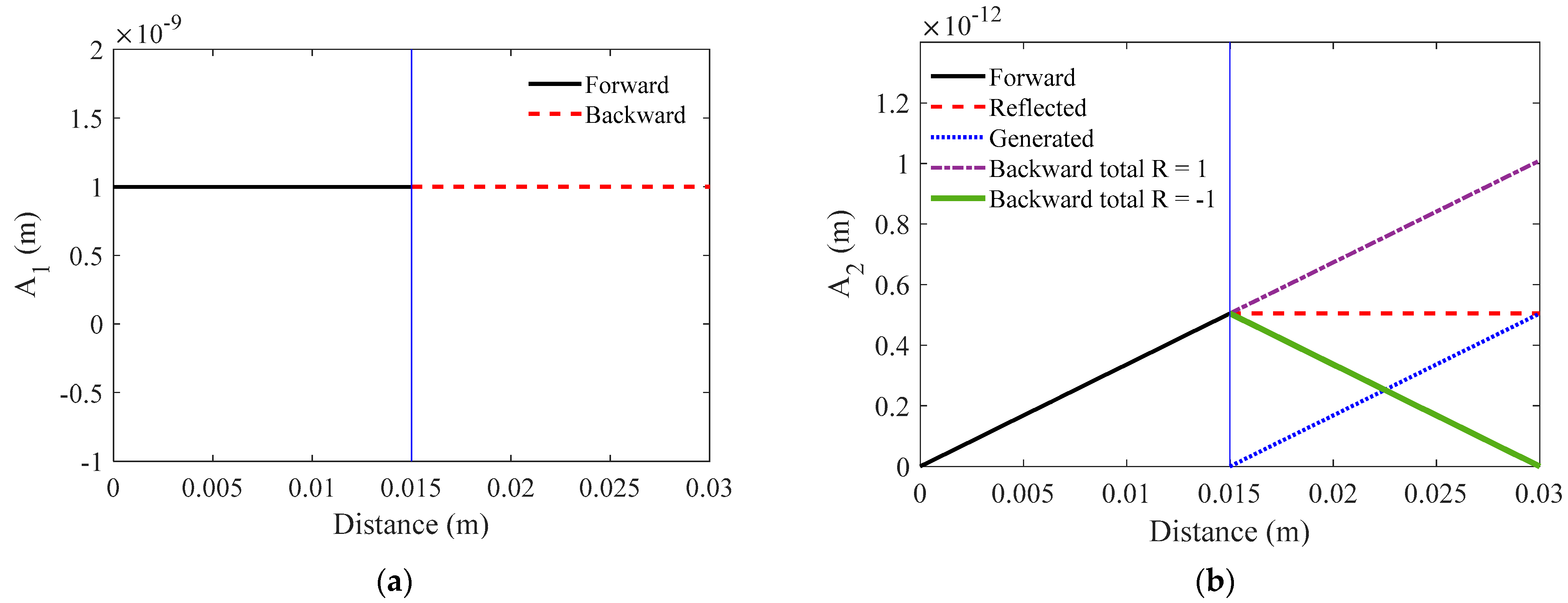
3.1. Pure Plane Wave

Figure 4 shows a schematic view in which the propagation process of a plane wave in the pulse-echo mode with a reflecting boundary is unfolded. When the calculation results are displayed in the pulse echo mode, the two propagation regions overlap, making it difficult to identify. Therefore, in Figure 4 and thereafter, the back propagation region is developed and spreads to the right side of the reflection boundary for convenience of observation.

The results of the pure longitudinal wave are presented here as references to other propagation and reflection problems. Plane waves are ideal waves without diffraction and attenuation. Figure 5 shows the variation in fundamental and second harmonic wave amplitudes in the forward and backward propagation directions. In the forward propagation, the displacement solution is given by Equation (2) for the fundamental and second harmonic waves. Since there is no diffraction and attenuation, the fundamental wave amplitude is constant, and the second harmonic amplitude linearly increases with propagation distance z.

The displacement solutions after reflection from the boundary are given by Equations (4) and (5), for the fundamental and second harmonic waves, respectively. Two kinds of boundary conditions are considered: the stress-free boundary ($R=-1$) and the rigid boundary ($R=1$). The same fundamental wave amplitudes are observed in Figure 5a after reflection from the rigid and stress-free boundaries because the reflection coefficient is $\left|R\right|=1$.

Figure 5b shows the reflected and newly generated second harmonic amplitudes and the total second harmonic amplitudes after being reflected from the two boundaries. The total second harmonic amplitude varies greatly depending on the boundary conditions used. It decreases linearly during backward propagation from the stress-free boundary and becomes 0 at the source position but continues to increase linearly in the case of the rigid boundary. This is known as the canceling and cumulative effects of the 2nd harmonic, respectively, which occur depending on the boundary conditions.

To illustrate the behavior of the received displacement, the phase before and after the boundary reflection was analyzed. The phase of the received wave was calculated by the function ${\varphi }_n(z)=\mathrm{ATAN}2\left(\mathrm{Im}(\tilde{v}(z)),\mathrm{Re}(\tilde{v}(z))\right), n=1,2$. The calculated phase angle was in the range of −π to π; therefore, 2π radians were inserted whenever there was a jump of more than 2π radians in order to make the phase spectrum continuous.

Figure 6 presents the phase calculation results for the fundamental and second harmonic waves. The phase of the fundamental wave in Figure 6a is continuous at the rigid boundary ($R=1$), while the reflected fundamental wave shows a phase difference of π after reflection at the stress-free boundary ($R=-1$). The continuous phase means that the reflected wave has the same sign of the incident wave. The π phase difference means that the reflected wave has the opposite sign of the incident wave. Note in Figure 6b that the phase of the reflected second harmonic is continuous at the rigid boundary ($R=1$), and the phase of the newly generated one is also continuous regardless of boundary conditions ($R=1$ or $R=-1$). On the other hand, the reflected second harmonic shows a phase difference of π after reflection at the stress-free boundary ($R=-1$). Therefore, the two second harmonic components will be added in the phase after reflection at the rigid boundary ($R=1$) and will cancel each other out after reflection at the stress-free boundary ($R=-1$).

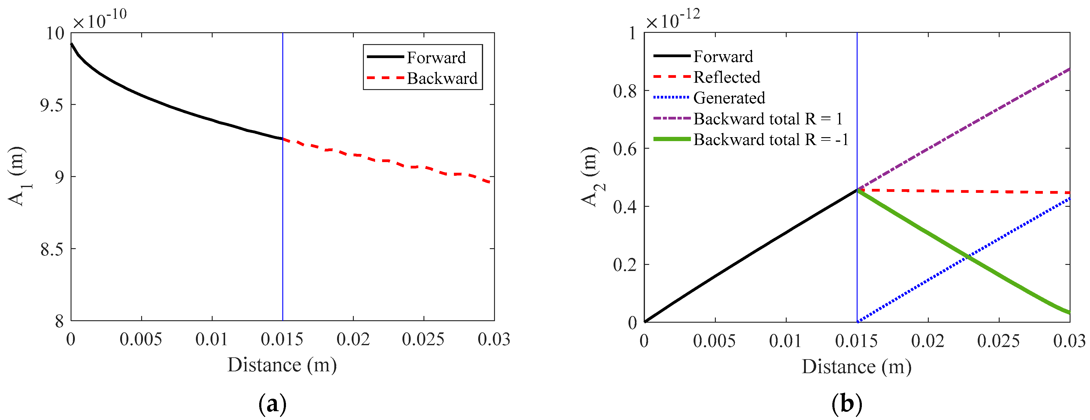
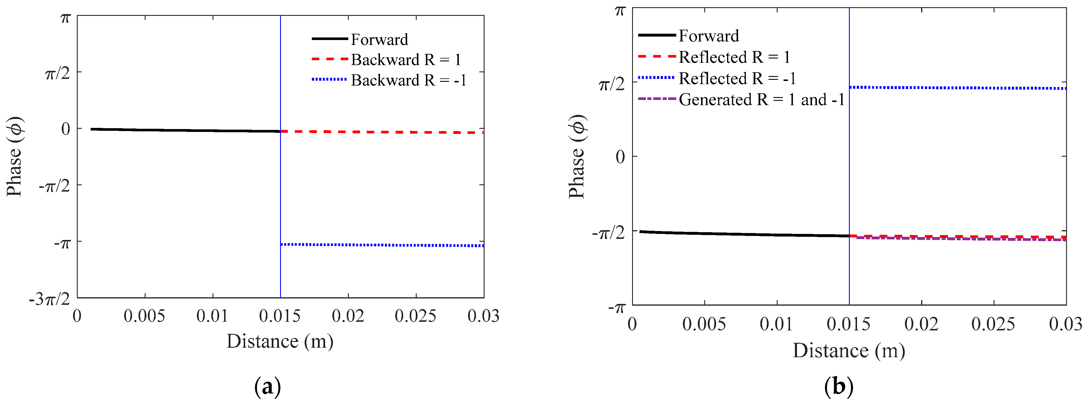
3.2. Single Element Transducer

Figure 7 shows the unfolded schematic of the longitudinal wave radiating from a single element transducer in the pulse-echo mode.

Figure 8 shows the received displacement amplitude of the fundamental and second harmonics for the single-element transducer. Note that the received displacement amplitude of the fundamental wave gradually decreases in Figure 8a. This behavior compares well with the behavior of the plane wave, where the received amplitude is constant at all distances (see Figure 5a). This is due to the diffraction effects of the finite size transducer in radiation and reception.

Figure 8b shows the received displacement amplitude of the second harmonic for rigid ($R=1$) and stress-free ($R=-1$) boundaries. The overall behavior of $R=-1$ is almost identical to that of the plane wave, except that the total second harmonic amplitude at the initial position does not completely disappear. This is due to the diffraction effect of the finite size transducer. It is noted that the results of $R=1$ continue to increase linearly. This is known as the cumulative effect of the second harmonic, which provides a major advantage in experimental measurement of the nonlinear effect [21]. The signal-to-noise ratio improves simply by letting the wave propagate for a longer distance.

The phase analysis results for the received displacement of Figure 8 are shown in Figure 9. Comparing Figure 9 to Figure 6, the results of the two cases are almost the same, so all discussions of Figure 6 can be applied to Figure 9. One thing to note is that the phase difference of the two second harmonic components for the stress-free boundary ($R=-1$) is not exactly π at the source position because of the diffraction effect.

3.3. Annular Array Transducer with Phase-Shifted Radiation

(1)

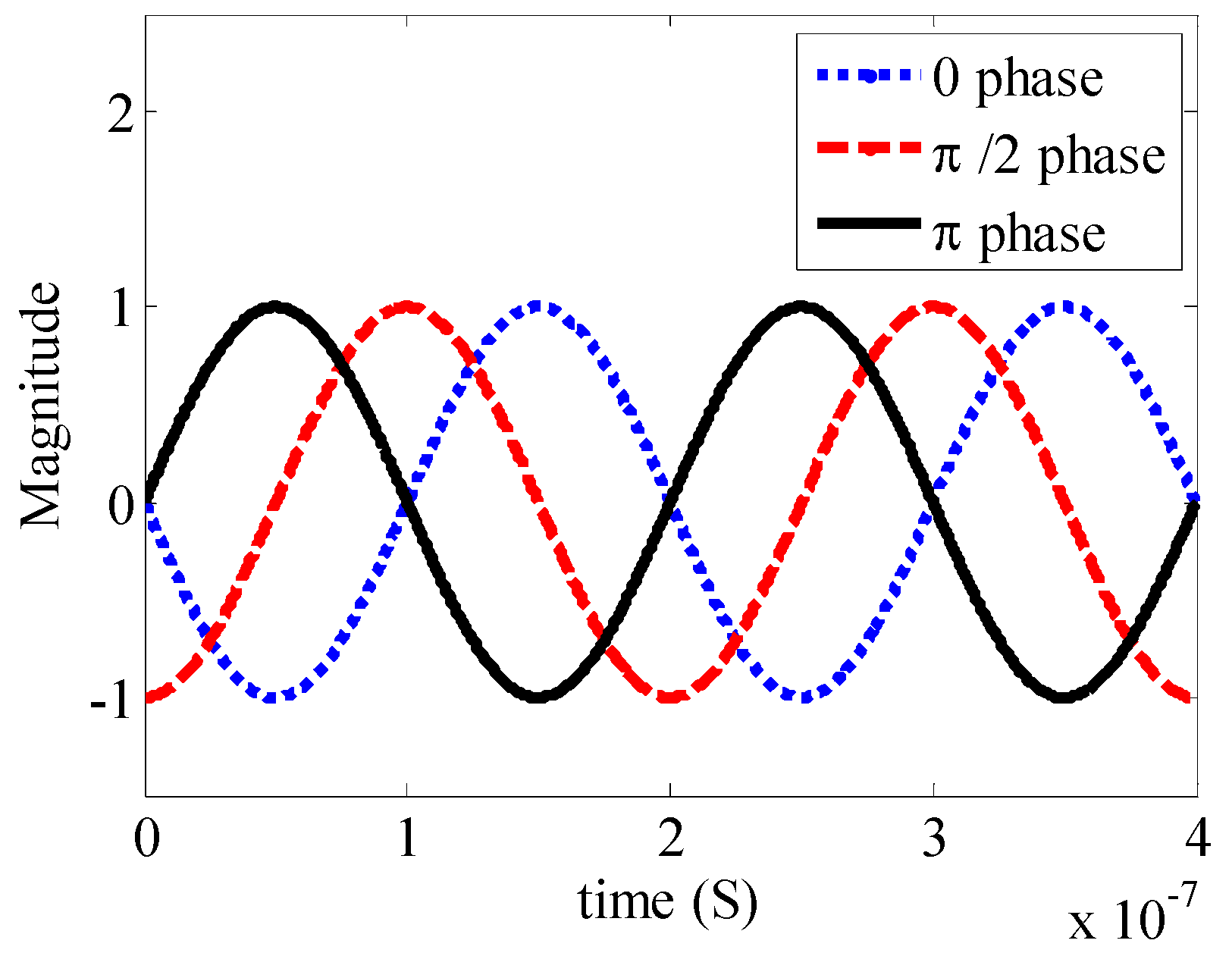
Phase shift of π between adjacent elements.

Figure 10 shows the unfolded schematic of longitudinal wave radiation from the four-element array transducer with the transmit phase shift of π radians between the elements and reception in the pulse-echo mode.

A phase shift technique can be applied to array transducers to improve SHG from the stress-free boundary. Here, the linear phase shifting is used for simulation, i.e., ${\varphi }^{(m)}=(m-1)\varphi$ where m denotes the element number and $\varphi$ represents the phase angle of the input signal. A schematic of the phase-shifted radiation is shown in Figure 10, where the phase difference of $\varphi =\pi$ between the elements is used and the simulation results are shown in Figure 11.

Figure 11 presents the distribution of the received displacement amplitude of the fundamental and second harmonics for the four-element transducer. The received fundamental wave amplitude is about half of that of the single-element transducer as shown in Figure 11a.

Figure 11b shows the received displacement amplitude of the second harmonic. The overall behavior looks much different from the single-element transducer of Figure 8b. The total second harmonic displacement amplitude decreases during backward propagation from the rigid boundary ($R=1$). On the other hand, it gradually increases during backward propagation from the stress-free boundary ($R=-1$) and exhibits weak cumulative behavior, achieving about 45% of the rigid boundary case of the single-element transducer at the source position. This is a big change achieved through the phase shift. As further studied below, one can optimize the amount of phase shift to apply to maximize second harmonic generation from the stress-free boundary.

The results of the phase analysis for the received displacement in Figure 11 are shown in Figure 12. For the fundamental wave of Figure 12a, the phase behavior is the same as in the previous two cases, so no further discussion is made here.

Figure 12b shows the phase analysis results of the second harmonic. The phase of the reflected second harmonic is continuous at the rigid boundary ($R=1$), and the phase difference with the newly generated one starts from about $2\pi /5$ at the boundary and gradually increases to about $7\pi /10$ at the source position. As a result, the total second harmonic displacement decreases as shown in Figure 11b. Conversely, the phase difference between the reflected and newly generated second harmonics gradually decreases from about $3\pi /5$ to about $3\pi /10$ for the stress-free boundary ($R=-1$). This is why the summed second harmonic amplitude increases slowly after reflection, as seen in Figure 11b.

(2)

Summary of phase−shifted simulation results.

Since the received fundamental and second harmonic amplitudes are highly dependent on the applied phase shift, the simulation was performed using more phase-shift values. A series of phase shifts were applied, using the linear phase between the adjacent elements as before, ${\varphi }^{(m)}=(m-1)\varphi$, where m denotes the element number and $\varphi$ represents the phase angle. Here, $\varphi$ ranges from 0 to π in π/20 increments.

The simulation results are presented in Figure 13. When there is no phase shift, the received amplitude of the four-element transducer is the same as the single-element transducer. The rigid boundary for the four-element transducer with zero phase shift corresponds to the through-transmission mode of thickness $z=2z_0$. It is noticed that the received fundamental wave amplitude does not depend on the boundary type.

The received second harmonic amplitudes resulting from the stress-free boundary are lower than those from the rigid boundary in most phase shift cases. However, in the last three cases of phase shifts (18π/20, 19π/20 and π) with the stress-free boundary, the received second harmonic amplitudes are larger than those of the rigid boundary, and the π phase shift provides the highest received amplitude. This amount of amplitude is about one order of magnitude larger than that of the single-element transducer with the stress-free boundary.

When the phase shift near π is applied, the phase difference between the reflected and newly generated second harmonic waves reach the minimum for the stress-free boundary. Therefore, the pulse-echo harmonic generation in this condition corresponds to the optimal condition, which is consistent with our previous research [28]. In this case, the first and third elements have the same phase, and the second and fourth elements have the same phase. This indicates that only two amplifiers are required in the experiment, even if a four-element array transducer is used.

4. Time Delay Focusing and Received Amplitudes

An annular array transducer that emits the longitudinal wave consists of a number of source elements and the radiation beam can be focused by applying an appropriate time delay to each element of the array transducer [29], as shown in Figure 14. A delay law for each element of the array transducer along the symmetry axis of the transducer with zero steering angle can be derived by considering the time-of-flight (TOF) from the centroid of each element to the specified focal distance F. The TOF difference between the mth element and the center element can be calculated as follows [30]:

$$\Delta t_m=\frac{r_m^2+r_{m+1}^2}{4cF}$$

(22)

where c is the longitudinal velocity of the sample, and $r_m$ and $r_{m+1}$ are the inner and outer radii of the mth element, respectively.

The delay of the time–domain signal is equivalent to multiplying the frequency domain signal by a phase term that is linear in frequency and proportional to its delay. If $F(\omega )$ is the Fourier transform (FT) of the time–domain signal $f(t)$, then the FT of the time shifted signal $f(t-\Delta t)$ can be obtained as $\exp (i\omega \Delta t)F(\omega )$, where $\Delta t$ is the time delay.

The array transducer used for a focused beam generation is the same as the four-element transducer, described before, used for phase-shifted radiation. The focal distance is set at the reflecting boundary of the sample (F = 15 mm) and the steering angle is 0°. In the simulation, the transmission time delay was calculated using Equation (22) and applied to focus the radiation beam at the specified focal distance. When calculating the received acoustic fields, the reception time delay was applied in the same way.

Figure 15 shows the received displacement amplitude of the fundamental and second harmonic waves when the radiation beam was focused at the reflecting boundary. Note that the received displacement amplitude of the fundamental wave fluctuates and increases very little in Figure 15a for both boundary conditions. This is due to the beam focusing of the array transducer. The boundary condition does not affect the calculated results of the fundamental wave. Figure 15b shows the received displacement amplitude of the second harmonic. In the back-propagation region, the rigid boundary yields a much larger SHG than the stress-free boundary. The stress-free boundary provides a relatively strong SHG, but the received amplitude initially tends to decrease due to the canceling effect and then accumulates during back propagation to the source location.

Figure 16a shows the phase analysis results of the fundamental wave, which are the same as before. Figure 16b shows the phase analysis results of the second harmonic. The phase of the reflected second harmonic is continuous at the rigid boundary ($R=1$), and the phase difference with the newly generated one starts from 0 at the boundary and gradually increases to about $\pi /5$ at the source position. As a result, the total second harmonic amplitude increases continuously as shown in Figure 15b. On the other hand, the phase difference between the reflected and newly generated second harmonics gradually increases from about $\pi$ to about $6\pi /5$ for the stress-free boundary ($R=-1$). This is why the summed second harmonic amplitude exhibits a sudden decrease at first and then a continuous increase, thereafter, as seen in Figure 15b.

5. Comparison of Simulation Results and discussion

5.1. Fundamental and Second Harmonic Amplitudes

Table 1. Summary of received displacement amplitudes in various simulation cases.

Type	Case No.	Phase Shift				Fundamental (10−10 m)	Second Harmonic (10−13 m)
		Disk	Annular Elements				Rigid	Stress-Free
Single element	1	-	-	-	-	8.95	8.82	0.31
Four element	2	0	π/4	2π/4	3π/4	3.78	1.39	0.16
	3	0	π/3	2π/3	π	1.62	1.31	0.34
	4	0	π/2	π	3π/2	1.33	4.51	0.71
	5	0	π	2π	3π	4.51	2.02	3.92
Dual element	6	0	π/2	-	-	2.93	7.23	0.88
	7	0	2π/3	-	-	5	4.18	0.67
	8	0	π	-	-	8.04	7.57	1.74
Focused	9	0	1.16π	3.10π	5.78π	4.94	4.09	1.98

lists the case numbers for various types of transducers and their received displacement amplitudes calculated in the pulse-echo (PE) mode, using two boundary conditions. The single element transducer is listed as Case 1. The single element transducer in the PE mode with the rigid boundary is the same as the through-transmission (TT) mode of thickness z = 2z₀. Four representative cases (2 to 5) are listed for the four-element array transducer with three different phase shifts applied. Three representative cases (6 to 8) are listed for the dual-element transducer with three different phase shifts applied. Finally, the focused transducer is included as Case 9, where the focal distance is set at the reflecting boundary of the sample. The single element transducer with the rigid boundary will be used as a reference in the comparison of received amplitudes in various cases.

Equation (11), for calculating the propagating sound beam fields, is called the Rayleigh–Sommerfeld (RS) integral and serves as the exact solution to the linear wave equation, Equation (9). Equation (12) also serves as an exact solution to the second harmonic wave equation in the quasilinear theory since the exact linear solution is used in the right hand-side of Equation (12). Therefore, all of the sound beam field equations derived in this study can be treated as exact solutions. Numerical calculations for the simulation were performed using MATLAB program. The amplitudes of the received displacements given in Table 1 can also be considered exact, although it may contain inherent errors that cannot be avoided in general numerical calculations.

First, it is noticed that the received fundamental amplitude does not depend on the type of boundary used (Case 1). This is because the magnitude of the received displacement, which is always positive, is calculated. The received fundamental and second harmonic amplitudes show a strong dependence on the applied phase shift (Case 2 to 8). The received amplitude also varies with the focal position [31], although the results of only one focal position are shown in this study (Case 9).

The single-element transducer with the rigid boundary (Case 1, $R=1$), which is equivalent to the through-transmission setup of propagation distance $2z_0$, provides the largest SHG. This is why such a pulse-echo setup is used to successfully measure the nonlinear parameter of fluids [7].

Table 1 shows the improvement of SHG through the phase shift of the multi-element array transducer, and the maximum second harmonic amplitude is obtained when the phase shift between the elements is π (Case 5, $R=-1$). The enhanced second harmonic generation also validates the determination of the nonlinear parameter, as further discussed below. The improved SHG in the dual-element transducer (Case 8, $R=-1$) is much weaker compared to the phase shift effect of the four-element transducer. These results indicate that the phase shift can be applied more effectively, using the four-element transducer to produce improved SHG in solid samples with stress-free boundaries.

The focusing of the incident beam at the reflecting surface (Case 9, $R=-1$) provides only slightly improved SHG, compared to the maximum possible SHG obtained by the phase-shift of the four-element transducer (Case 5, $R=-1$). This can be attributed to the insufficient number of transmission elements that cannot achieve very tight focusing. A 64-element linear array probe or a spherically focused probe provides tight focusing to achieve the maximum possible SHG, with the phase difference between the two second harmonic components reaching about π/2 [26,27].

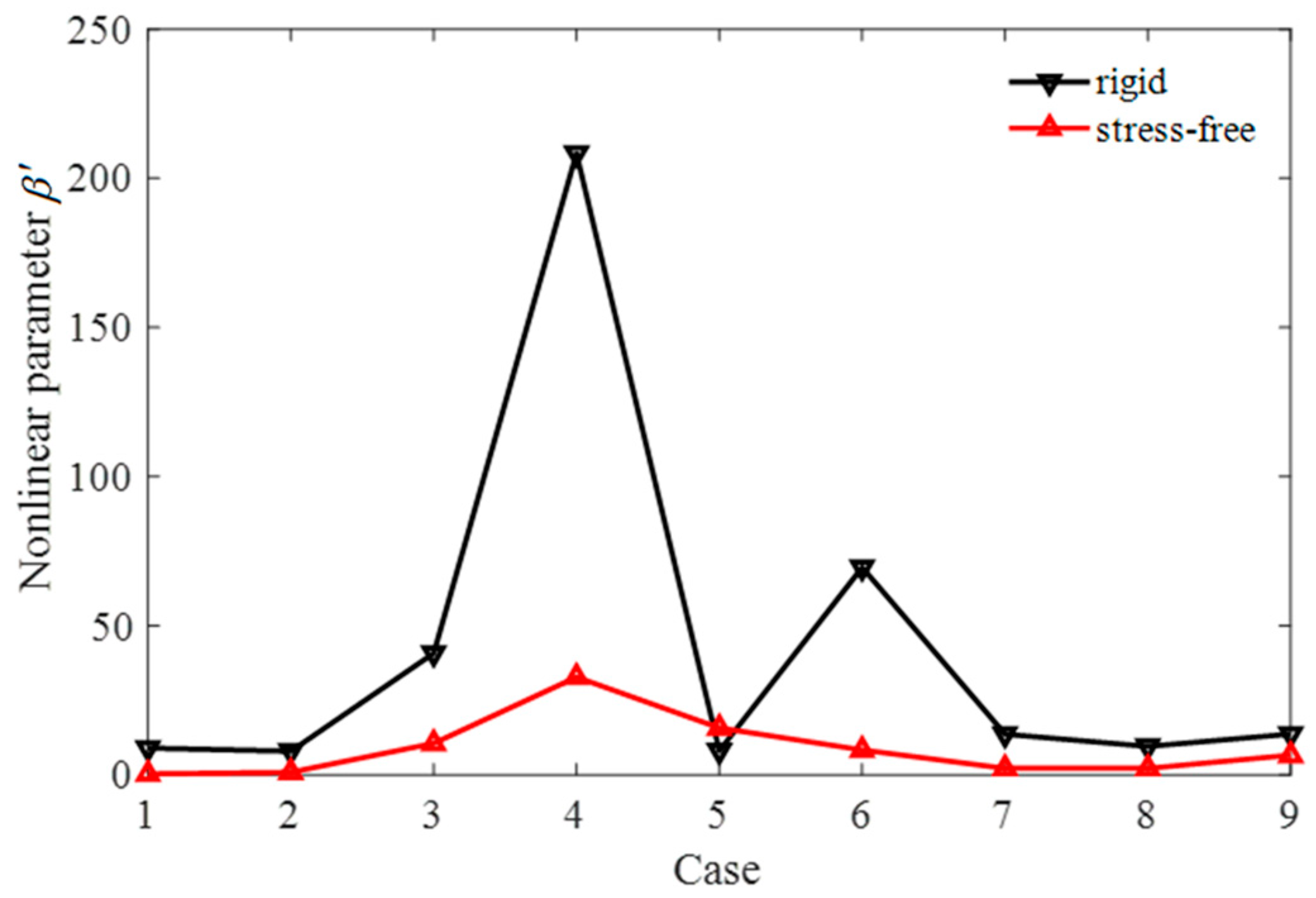
5.2. Uncorrected Nonlinear Parameter

The material nonlinearity is frequently quantified by the “absolute” nonlinear parameter, $\beta$, which is defined by Equation (3). However, in practical experiments, the “uncorrected” nonlinear parameter of Equation (18) is measured using finite size transducers. In this case, in order to determine the $\beta$, corrections for diffraction effects and material attenuation are required. In pulse-echo mode experiments, additional correction for boundary reflection is required.

The ${\beta }^{\prime }$ was calculated using the data of Table 1 and is presented in Figure 17. Case 5 with $R=-1$ shows a relatively high ${\beta }^{\prime }$ because it yields the largest second harmonic amplitude. In fact, the calculated ${\beta }^{\prime }$ is about three times larger than the reference $\beta$, so a small correction value much lower than 1 is required. This case may be a possible option for an accurate measurement of $\beta$, but it is not the best option. The focused transducer (Case 9, $R=-1$) may be a better choice because it gives a reasonable ${\beta }^{\prime }$ resulting from the improved SHG and requires a correction value close to 1. When a phase shift is accompanied for the measurement of ${\beta }^{\prime }$ only with $R=-1$, it seems that Cases 3 and 6 are suitable choices. The optimal phase shift criterion for the reliable determination of $\beta$ using the four-element transducer is to maximize SHG from the stress-free boundary and to minimize the dependence on the correction by making the correction value as close to one as possible. It is noted that the largest value of ${\beta }^{\prime }$ occurs when $R=1$ in Case 4 because the second harmonic amplitude is relatively large, and the fundamental wave amplitude is the smallest.

The simulation results observed here show that the transmission phase shift can be a useful tool in the pulse-echo SHG of relatively thin solid samples with stress−free boundaries. The design of array transducers and the amount of phase shift to apply for a given material and frequency can be optimized in terms of maximum possible SHG or in terms of the more accurate determination of $\beta$.

The current work covers ideal cases, but the actual phenomenon will not differ much from the theoretical investigation presented here. Future work should be able to include laboratory verification and field verification. Some of the challenges associated with experimental validation are making such a multiple element transducer. It should be able to carry high power input signals with minimal source harmonics. All elements of the transducer should be able to act as both a transmitter and a receiver and need to have a wide bandwidth to cover both the fundamental and second harmonic frequency components. In addition, at least four channels of function generators and high-power amplifiers may be required.

This study deals with the generation of second harmonic in relation to the evaluation of the properties of nonlinear solid materials. Just as the nonlinear image based on the second harmonic is superior to the linear image, the third harmonic image can have a better resolution in tissue characterization because the main lobe is narrower in the transverse beam pattern than in the second harmonic. A measure of the third harmonic is the nonlinear coefficient C/A in fluids and biological media. Other studies have shown that the third harmonic is more sensitive to microstructure changes than the second harmonic by measuring the amplitude of the third harmonic or measuring the relative third-order nonlinear parameter for the damaged solid medium [32].

6. Conclusions

In this work, we studied a novel phase shift technique to enhance SHG reflected at the stress−free boundaries of thin solid samples, using annular array transducers. The received second harmonic amplitudes generated from various sound sources were compared through simulation, and their phase characteristics were analyzed. Based on the simulation results, the following conclusions are drawn:

(1)

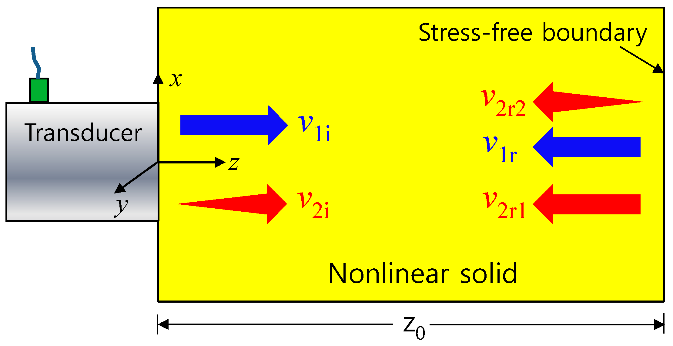
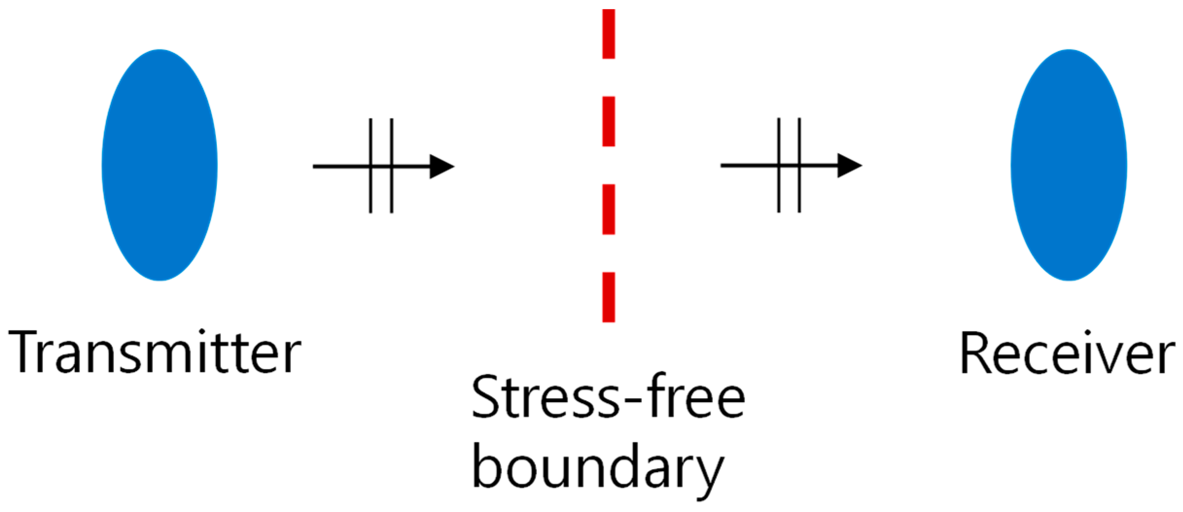
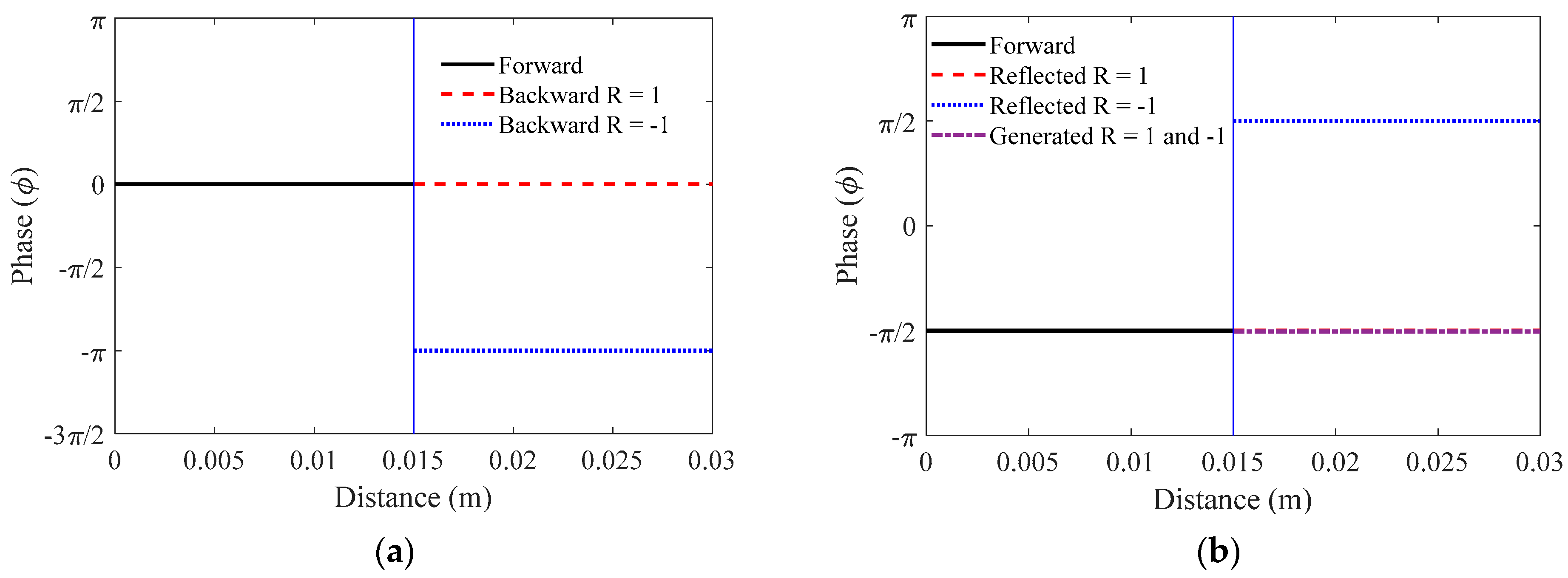
Plane or diffracted waves emitted by single−element transducers are difficult to use to generate second harmonic amplitudes or to measure the nonlinear properties of solids in the pulse-echo mode. This is because the two components of the second harmonic are out of phase with each other and cancel at the receiver position.

(2)

The transmission phase shift can be a useful tool in the pulse-echo SHG of relatively thin samples. Moreover, the design of four−element transducers can be optimized in terms of shape and size along with the amount of phase shift to obtain the maximum possible SHG. Array transducers with four elements offer distinct advantages over two elements, as they give more options when applying the phase shift or adjusting the focal length.

(3)

To measure the nonlinear parameter (β) of a specimen with much improved second harmonic amplitude, compared to a single element transducer, a four−element array transducer using a beam focused at the specimen boundary may be a good alternative.

References

1. Achenbach, J. Quantitative nondestructive evaluation. Int. J. Solids Struct. 2000, 37, 13–27. [Google Scholar] [CrossRef]
2. Kim, C.; Park, I. Microstructural degradation assessment in pressure vessel steel by harmonic generation technique. J. Nucl. Sci. Technol. 2008, 45, 1036–1040. [Google Scholar] [CrossRef]
3. Viswanath, A.; Rao, B.P.C.; Mahadevan, S.; Jayakumar, T.; Raj, B. Microstructural characterization of M250 grade maraging steel using nonlinear ultrasonic technique. J. Mater. Sci. 2010, 45, 6719–6726. [Google Scholar] [CrossRef]
4. Hurley, D.C.; Balzar, D.; Purtscher, P.T. Nonlinear ultrasonic assessment of precipitation hardening in ASTM A710 steel. J. Mater. Res. 2000, 15, 2036–2042. [Google Scholar] [CrossRef]
5. Cantrell, J.H.; Yost, W.T. Effect of precipitate coherency strains on acoustic harmonic generation. J. Appl. Phys. 1997, 81, 2957–2962. [Google Scholar] [CrossRef]
6. Zheng, Y.; Maev, R.G.; Solodov, I.Y. Nonlinear acoustic applications for material characterization: A review. Can. J. Phys. 1999, 77, 927–967. [Google Scholar] [CrossRef]
7. Meulen, F.V.; Haumesser, L. Evaluation of B/A nonlinear parameter using an acoustic self-calibrated pulse-echo method. Appl. Phys. Lett. 2008, 92, 214106. [Google Scholar] [CrossRef]
8. Chakrapani, S.K.; Barnard, D.J. A calibration technique for ultrasonic immersion transducers and challenges in moving to-wards immersion based harmonic imaging. J. Nondestruct. Eval. 2019, 38, 76. [Google Scholar] [CrossRef]
9. Cho, S.; Jeong, H.; Zhang, S.; Li, X. Dual element transducer approach for second harmonic generation and material nonlinearity measurement of solids in the pulse echo method. J. Nondestruct. Eval. 2020, 39, 62. [Google Scholar] [CrossRef]
10. Jeong, H.; Cho, S.; Shin, H.; Zhang, S.; Li, X. Optimization and Validation of Dual Element Ultrasound Transducers for Improved Pulse-echo Measurements of Material Nonlinearity. IEEE Sens. J. 2020, 20, 13596–13606. [Google Scholar] [CrossRef]
11. Kim, J.; Song, D.-G.; Jhang, K.-Y. A method to estimate the absolute ultrasonic nonlinearity parameter from relative measure-ments. Ultrasonics 2017, 77, 197–202. [Google Scholar] [CrossRef]
12. Torello, D.; Thiele, S.; Matlack, K.H.; Kim, J.-Y.; Qu, J.; Jacobs, L.J. Diffraction, attenuation, and source corrections for nonlinear Rayleigh wave ultrasonic measurements. Ultrasonics 2015, 56, 417–426. [Google Scholar] [CrossRef] [Green Version]
13. Zhang, S.; Li, X.; Jeong, H.; Hu, H. Modeling nonlinear Rayleigh wave fields generated by angle beam wedge transducers—A theoretical study. Wave Motion 2016, 67, 141–159. [Google Scholar] [CrossRef]
14. Zhang, S.; Li, X.; Chen, C.; Jeong, H.; Xu, G. Characterization of Aging Treated 6061 Aluminum Alloy Using Nonlinear Rayleigh Wave. J. Nondestruct. Eval. 2019, 38, 88. [Google Scholar] [CrossRef]
15. Hong, M.; Su, Z.; Wang, Q.; Cheng, L.; Qing, X. Modeling nonlinearities of ultrasonic waves for fatigue damage characteriza-tion: Theory, simulation, and experimental validation. Ultrasonics 2014, 54, 770–778. [Google Scholar] [CrossRef]
16. Xiang, Y.; Deng, M.; Xuan, F.-Z.; Liu, C.-J. Cumulative second-harmonic analysis of ultrasonic Lamb waves for ageing behavior study of modified-HP austenite steel. Ultrasonics 2011, 51, 974–981. [Google Scholar] [CrossRef]
17. Zhu, W.; Xiang, Y.; Liu, C.-J.; Deng, M.; Ma, C.; Xuan, F.-Z. Fatigue Damage Evaluation Using Nonlinear Lamb Waves with Quasi Phase-Velocity Matching at Low Frequency. Materials 2018, 11, 1920. [Google Scholar] [CrossRef] [Green Version]
18. Christopher, T. Experimental investigation of finite amplitude distortion-based, second harmonic pulse echo ultrasonic imaging. IEEE Trans. Ultrason. Ferroelectr. Freq. Control 1998, 45, 158–162. [Google Scholar] [CrossRef]
19. Makin, I.R.S.; Averkiou, M.A.; Hamilton, M.F. Second-harmonic generation in a sound beam reflected and transmitted at a curved interface. J. Acoust. Soc. Am. 2000, 108, 1505–1513. [Google Scholar] [CrossRef]
20. Chitnalah, D.K.; Jakjoud, H.; Nadi, M. Pulse echo method for nonlinear ultrasound parameter measurement. Tech. Acoust. 2007, 13, 1–8. [Google Scholar]
21. Jeong, H.; Cho, S.; Zhang, S.; Li, X. Acoustic nonlinearity parameter measurements in a pulse-echo setup with the stress-free reflection boundary. J. Acoust. Soc. Am. 2018, 143, EL237–EL242. [Google Scholar] [CrossRef]
22. Thompson, D.O.; Tennison, M.A.; Buck, O. Reflections of harmonics generated by finite-amplitude waves. J. Acoust. Soc. Am. 1968, 44, 435–436. [Google Scholar] [CrossRef]
23. Bender, F.A.; Kim, J.-Y.; Jacob, L.J.; Qu, J. The generation of second harmonic waves in an isotropic solid with quadratic non linearity under the presence of a stress free boundary. Wave Motion 2013, 50, 146–161. [Google Scholar] [CrossRef]
24. Best, S.R.; Croxford, A.J.; Neild, S.A. Pulse-echo Harmonic Generation Measurements for Non-destructive Evaluation. J. Nondestruct. Eval. 2014, 33, 205–215. [Google Scholar] [CrossRef] [Green Version]
25. Liu, Y.; Li, X.; Zhang, G.; Zhang, S.; Jeong, H. Characterizing Microstructural Evolution of TP304 Stainless Steel Using a Pulse-echo Nonlinear Method. Materials 2020, 13, 1395. [Google Scholar] [CrossRef] [Green Version]
26. Jeong, H.; Zhang, S.-Z.; Li, X.-B. Second-harmonic generation in focused beam fields of phased-array transducers in a nonlinear solid with a stress-free boundary. Transp. Saf. Environ. 2019, 1, 117–125. [Google Scholar] [CrossRef]
27. Zhang, S.; Li, X.; Jeong, H.; Cho, S.; Hu, H. Theoretical and experimental investigation of the pulse-echo nonlinearity acoustic sound fields of focused transducers. Appl. Acoust. 2017, 117, 145–149. [Google Scholar] [CrossRef]
28. Jeong, H.; Zhang, S.; Li, X. Improvement of pulse-echo harmonic generation from stress-free boundary through phase shift of a dual element transducer. Ultrasonics 2018, 87, 145–151. [Google Scholar] [CrossRef]
29. Hazard, C.; Fisher, R.; Mills, D.; Smith, L.; Tbomemus, K.; Wodnicki, R. Annular array beamforming for 2D arrays with reduced system channels. In Proceedings of the 2003 IEEE Ultrasonics Symposium, Honoluludoi, HI, USA, 5–8 October 2003; pp. 1859–1862. [Google Scholar] [CrossRef]
30. Liaptsis, G.; Liaptsis, D.; Wright, B.; Charlton, P. Focal law calculations for annular phased array transducers. e-J. NDT 2015, 20, 1–7. [Google Scholar]
31. Cho, S.; Jeong, H.; Park, I.K. Optimal Design of Annular Phased Array Transducers for Material Nonlinearity Determination in Pulse–Echo Ultrasonic Testing. Materials 2020, 13, 5565. [Google Scholar] [CrossRef]
32. Abeele, K.V.D.; Breazeale, M.A. Theoretical model to describe dispersive nonlinear properties of lead zirconate–titanate ceramics. J. Acoust. Soc. Am. 1996, 99, 1430–1437. [Google Scholar] [CrossRef]
Figure 1. Schematic of a pulse-echo testing configuration with a stress-free boundary.
Applsci 11 04836 g001
Figure 2. Examples of transducers used for simulation of second harmonic generation in the pulse-echo setup: (a) single element, (b) four−element annular array, and (c) dual-element annular array.
Applsci 11 04836 g002
Figure 3. Illustration of phase shift.
Applsci 11 04836 g003
Figure 4. Unfolded schematic of plane longitudinal wave propagation in the pulse-echo mode.
Applsci 11 04836 g004
Figure 5. Changes in the amplitude of displacement received from plane wave propagation: (a) fundamental wave and (b) second harmonic wave. The vertical line in each figure denotes the location of the reflection boundary.
Applsci 11 04836 g005
Figure 6. Phase analysis results of Figure 5: (a) fundamental wave, and (b) second harmonic wave.
Applsci 11 04836 g006
Figure 7. Longitudinal wave propagation from a single−element transducer and reception in the pulse-echo mode.
Applsci 11 04836 g007
Figure 8. Changes in the amplitude of displacement received from the single-element transducer: (a) fundamental wave and (b) second harmonic wave.
Applsci 11 04836 g008
Figure 9. Phase analysis results of Figure 8: (a) Fundamental wave and (b) second harmonic wave.
Applsci 11 04836 g009
Figure 10. Phase−shifted radiation of π between the elements of the annular array transducer and reception in the pulse-echo mode.
Applsci 11 04836 g010
Figure 11. Changes in the amplitude of displacement received from phase−shifted radiation of π: (a) fundamental wave and (b) second harmonic wave.
Applsci 11 04836 g011
Figure 12. Phase analysis results of Figure 11: (a) fundamental wave and (b) second harmonic wave.
Applsci 11 04836 g012
Figure 13. Amplitude of the received displacement as a function of the phase shift between the array transducer elements: (a) fundamental wave, and (b) second harmonic wave.
Applsci 11 04836 g013
Figure 14. Conventional time delay focusing of the four-element array transducer and reception in the pulse-echo mode.
Applsci 11 04836 g014
Figure 15. Changes in the amplitude of displacement received from conventional time delay focusing: (a) fundamental wave and (b) second harmonic wave.
Applsci 11 04836 g015
Figure 16. Phase analysis results of Figure 15: (a) fundamental wave and (b) second harmonic wave.
Applsci 11 04836 g016
Figure 17. Comparison of uncorrected nonlinear parameter β for various simulation cases.
Applsci 11 04836 g017