A Novel Shape Finding Method for the Main Cable of Suspension Bridge Using Nonlinear Finite Element Approach

Featured Application

This study proposed a novel shape finding technique for both the 2D parallel and 3D spatial main cables of suspension bridge with sufficient accuracy and high efficiency.

Abstract

The determination of the final cable shape under the self-weight of the suspension bridge enables its safe construction and operation. Most existing studies solve the cable shape segment-by-segment in the Lagrangian coordinate system. This paper develops a novel shape finding method for the main cable of suspension bridge using nonlinear finite element approach with Eulerian description. The governing differential equations for a three-dimensional spatial main cable is developed before a one-dimensional linear shape function is introduced to solve the cable shape utilizing the Newton iteration method. The proposed method can be readily reduced to solve the two-dimensional parallel cable shape. Two iteration layers are required for the proposed method. The shape finding process has no need for the information of the cable material or cross section using the present technique. The commonly used segmental catenary method is compared with the present method using three cases study, i.e., a 1666-m-main-span earth-anchored suspension bridge with 2D parallel and 3D spatial main cables as well as a 300-m-main-span self-anchored suspension bridge with 3D spatial main cables. Numerical studies and iteration results show that the proposed shape finding technique is sufficiently accurate and operationally convenient to achieve the target configuration of the main cable.

1. Introduction

The advancements of the fundamental theory, construction technique, and new materials have enabled the rapid growth of the bridge main span length to cross the large rivers, wide canyons, and deep straits [1]. As a bridge type with largest span capacity, the suspension bridge is always a preferable candidate for a single span longer than one kilometer from the perspectives of the mechanical property and economic performance. Though the longest suspension bridge is still the Akashi Kaikyō Bridge with main span of 1991 m built in 1998, several super-long suspension bridges with the main span longer than two kilometers are recently being constructed, such as the 2023-m-main-span Çanakkale 1915 Bridge in Turkey, the 2018-m-main-span Shiziyang Bridge in China, and the 2300-m-main-span Zhanggao Bridge across Yangtze River in China. The gravity stiffness of the main cable owing to the self-weight or initial tension stress is one of the most important reasons for the continuous growth of the main span for the suspension bridge. Its proportion in the stiffness of the suspension bridge system will also increase with the growth of the main span length.

Essentially, the gravity stiffness steams from the geometric nonlinearity, which strongly depends on the configuration and internal force of the main cable. However, the shape of the main cable should be prescribed accounting for the effects of all external forces, which is always unable to be amended during the construction [2]. The configuration or target shape for the main cable at the initial equilibrium state under dead loads due to the self-weights of the bridge should be predetermined at the preliminary design stage. A shape finding or form finding process is therefore conducted to determine the shape and internal forces of the main cable through minimizing the dead-load-induced deformation of the bridge. Moreover, the increase of the main cable dimension and the reduction of the cable design safety factor require a more refined estimation of the cable configuration and internal forces in the structural components [3].

In the past several decades, the theory of the shape finding for the main cable of suspension bridge has received intensive attention. For a given cable segment of specified unstrained length, cross section area, Young’s elastic modulus, and density, there are many kinds of relations between node force and node displacement/position, e.g., a link element considering sag effect [4,5], a two-node curved cable element [6,7], and various two-dimensional [8] and three-dimensional catenary cable elements [9,10,11,12]. The segmental parabola theory assumes the shape of the main cable to be a parabolic curve under uniform load [4], [13]. This approximation ignores the concentrated forces transferred from the hangers, which is only acceptable for medium and small span suspension bridges.

The segmental catenary theory allows one to achieve the analytical solutions of each cable segment shape. The equations describing the analytical relations between the axial forces and the strained/unstrained lengths of a cable segment under the action of the self-weight can be found in many pioneering studies, e.g., [14]. These equations were then widely employed to develop various shape finding approaches for the main cable of the suspension bridge, such as the initial force method or segmental catenary method (SCM) [3,15,16,17,18], the target configuration under dead load (TCUD) method [19], the improved TCUD method [20], the Generalized TCUD method [21], the coordinate iteration method [22], and the perturbation approach [23,24]. The unstrained length of each main cable segment in these methods is unknown and solved in the successive nonlinear equations using the nonlinear finite element iteration [15,16,25,26,27,28,29]. Generally, at least two loop layers are required for calculating the unstrained length and axial force of each catenary segment before determining the shape of the main cable. To avoid a loop over each element, the unstrained length of each cable is treated as an unknown parameter in formulating a tangential stiffness matrix in the TCUD method [19] and the Generalized TCUD method [21]. Shape finding process based on the analytical solution of each catenary element is mostly exact. However, its theoretical derivation is complex, and the achievement of the algorithm requires high programing skills. Moreover, most of them are restricted to two-dimensional (2D) parallel main cables.

The three-dimensional (3D) spatial main cables, which are intended to enhance the lateral stiffness of the suspension bridge, have been employed in some recent projects, such as the Yongjong Grand Bridge in Korea, Jiangdong Bridge in China, the New Oakland Bay Bridge in the USA, and Halogaland Bridge in Norway. Tang et al. [25] extended the 2D segmental catenary approach to 3D by iterating the axial component of the main cable to achieve a target sag-to-span ratio. Kim et al. [20] estimated the spatial cable shape of the Yongjong Grand Bridge using an improved TCUD method coupled with the initial force method by introducing a 3D elastic catenary cable element. The procedures in these studies are lengthier and more time-consuming for spatially curved cables as compared with the planar cable system.

To simplify the calculation procedure and reduce the computation burden, the finite element method (FEM) was employed to estimate the 3D main cable shape. A five-step algorithm was proposed in Xiao et al. [30] and Song et al. [31] using the common FEM software ANSYS to solve both 2D planar and 3D spatial cable shapes, which is convenient to be executed at the preliminary design stage. However, the use of the common FEM program results in the insufficiently theoretical analysis for the core algorithm.

As can be seen, most above-mentioned methods are developed in the Lagrangian coordinate system, which expresses the quantities of interest as the function of the undeformed position or unstrained length of the main cable segment. However, the unstrained length of each cable segment is usually unknown, resulting in more loop layers. In this paper, a shape finding procedure for the main cable using the NFEM and the Eulerian description is developed. A modified governing equation for the whole main cable, rather than cable segments, based on the force equilibrium is proposed by introducing a condition function to express the concentrated forces from hangers [14]. All quantities of the main cable are expressed in a fixed coordinate system. That is, if the longitudinal direction along the bridge axis, the vertical and lateral directions of a suspension bridge are defined as the x-, y- and z-axes, the variables of the main cable related to the y and z coordinates of the cable are expressed by a fixed x coordinate instead of the unstrained length of the cable. An FEM discretization process [32] starting from a linear basic function is then conducted to solve the governing partial differential equations to get a group of nonlinear algebraic equations. The iteration schemes for solving the cable shape with known and unknown horizontal axial force are proposed. The commonly used segmental catenary method is compared with the present approach. The shapes of 2D parallel and 3D spatial main cables, which are applied to a 1666-m main span earth-anchored suspension bridge are solved using the present approach and the segmental catenary method, respectively. The self-anchored Yongjong Grand Bridge analyzed by Kim et al. [16] is also examined using the proposed method to validate its accuracy. The proposed algorithm provides an alternative to estimate the main cable shape at the preliminary design stage using only two-layer iteration and less programming. The use of the FEM allows the present method to be readily embedded in some commonly used FE analysis software and easily used by general bridge engineers.

2. Shape Finding of the Main Cable with Eulerian Description

2.1. Governing Equations of Spatial Main Cable

As shown in Figure 1a, a spatial main cable is described in a Eulerian coordinate system. The x-axis is the longitudinal direction along the bridge axis. The y-axis is in the vertical direction and the z-axis is in the lateral direction of the bridge. The tension forces of the cable at two ends are decomposed into three components, i.e., $\left(H_0,F_{y1},F_{z1}\right)$ and $\left(H_0,F_{y2},F_{z2}\right)$. The unit weight of the main cable is defined as q. The projected length of the cable in the x-direction is L. The total number of hangers is n. The tension of ith (i = 1, 2, …, n) inclined hanger is noted as $T_i$, which consists of a vertical force of $T_{yi}$ in the y-direction and a lateral component of $T_{zi}$ in the z direction, as shown in Figure 1b. The connection position between the ith hanger and the main cable is at the coordinate of $\left(x_i,y_i,z_i\right)$ or $\left(x_i,y_i,-z_i\right)$. The other connection position at the bridge deck is defined as $\left(x_i,y_{di},z_{di}\right)$ or $\left(x_i,y_{di},-z_{di}\right)$.

At the final state of the bridge, the lumped force transferred from each inclined hanger $T_i$ can be determined from the dead load of the girder and self-weight of the hanger [25]. The distribution force due to the gravity of the main cable are also prescribed. To establish the equilibrium equations of a spatial main cable, four assumptions are employed in this study:

(1)

The main cable of the suspension bridge is ideally flexible and unable to bear any bending moment. Only the axial tension is considered for the main cable.

(2)

The axial deformation of the main cable is tiny such that the area of the cross section for the main cable remains unchanged and the cable weight per unit length is a constant.

(3)

The linear elastic assumption for all materials is adopted.

(4)

All the loadings on the main cable are parallel to the y-o-z plane. The tension in the x-direction of the main cable is constant and defined as $H_0$.

The first three assumptions are commonly employed during the shape finding process at the preliminary design stage, e.g., Li et al. [12]; Kim et al. [16,20]; Zhang et al. [18]. As reported by Zhang et al. [18], the flexural stiffness of the main cable is insignificant and can be neglected during the construction process. Moreover, the main cable should work substantially below the yield stress such that the axial deformation is tiny and the variation of the cross-section area is negligible. For most modern suspension bridges, the hangers in are designed to incline only in the cross-sectional plane of the bridge. There is no or insignificant tension component of each hanger along the longitudinal direction. Therefore, the tension of the main cable in the x-direction remains constant.

The tension force along the axis of the main cable is assumed as $\mathit{F}$, which can be decomposed into the $H_0$, $F_y$ and $F_z$ in the x-, y- and z-direction, respectively. The direction of $\mathit{F}$ is parallel to the cable element at the position of interest, i.e., $d\mathit{s}=\left(dx, dy, dz\right)$. The ratio between the $F_y$, $F_z$ and $H_0$ can be expressed as:

$$\frac{F_y}{H_0}=\frac{dy}{dx}$$

(1)

$$\frac{F_z}{H_0}=\frac{dz}{dx}$$

(2)

Taking the derivative of Equations (1) and (2) with the respect to $x$ gives the form of

$$\frac{d{F}_y}{dx}=H_0\frac{d^{2}y}{d{x}^2}$$

(3)

$$\frac{d{F}_z}{dx}=H_0\frac{d^{2}z}{d{x}^2}$$

(4)

The distributions of $F_y$ and $F_z$ along the x-direction can also be formulated as the functions of real loadings:

$$\frac{d{F}_y}{dx}=q\sqrt{1+{\left(\frac{dy}{dx}\right)}^2+{\left(\frac{dz}{dx}\right)}^2}+T_{yi}\delta \left(x-x_i\right)$$

(5)

$$\frac{d{F}_z}{dx}=T_{zi}\delta \left(x-x_i\right)$$

(6)

in which $\delta \left(x-x_i\right)$ is a condition function defined as:

$$\delta \left(x-x_i\right)=\{\begin{array}{c}\infty ,x=x_i\\ 0,x\ne x_i\end{array}$$

(7)

$${{\displaystyle \int }}_{-\infty }^{+\infty }f\left(x\right)\delta \left(x-x_i\right)dx=f\left(x_i\right)$$

(8)

It is noteworthy that the Einstein summation convention is employed hereafter in this study for the purpose of the formula simplification, e.g., $T_{yi}\delta \left(x-x_i\right)={{\displaystyle \sum }}_{i=1}^n{T}_{yi}\delta \left(x-x_i\right)$ in Equations (5) and (6). The governing equations for the spatial main cable can be obtained by combing the Equations (3) and (6) with the form of

$$H_0{y}^{″}=q\sqrt{1+{y^{\prime }}^2+{z^{\prime }}^2}+T_{yi}\delta \left(x-x_i\right)$$

(9)

$$H_0{z}^{″}=T_{zi}\delta \left(x-x_i\right)$$

(10)

in which the dash denotes spatial differentiation with respect to $x$. For the two-dimensional main cable that is parallel to the x-o-y plane, a constant z coordinate is assigned. Equations (9) and (10) can be reduced as:

$$H_0{y}^{″}=q\sqrt{1+{y^{\prime }}^2}+T_{yi}\delta \left(x-x_i\right)$$

(11)

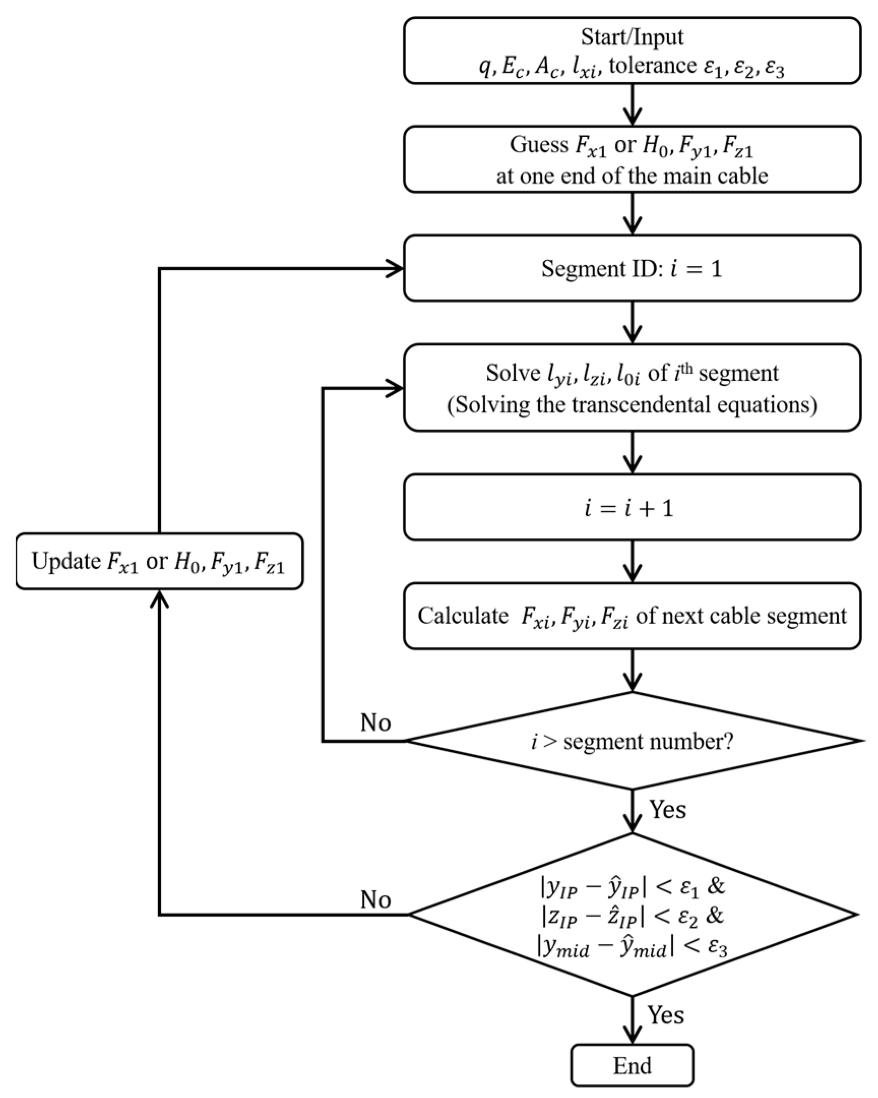
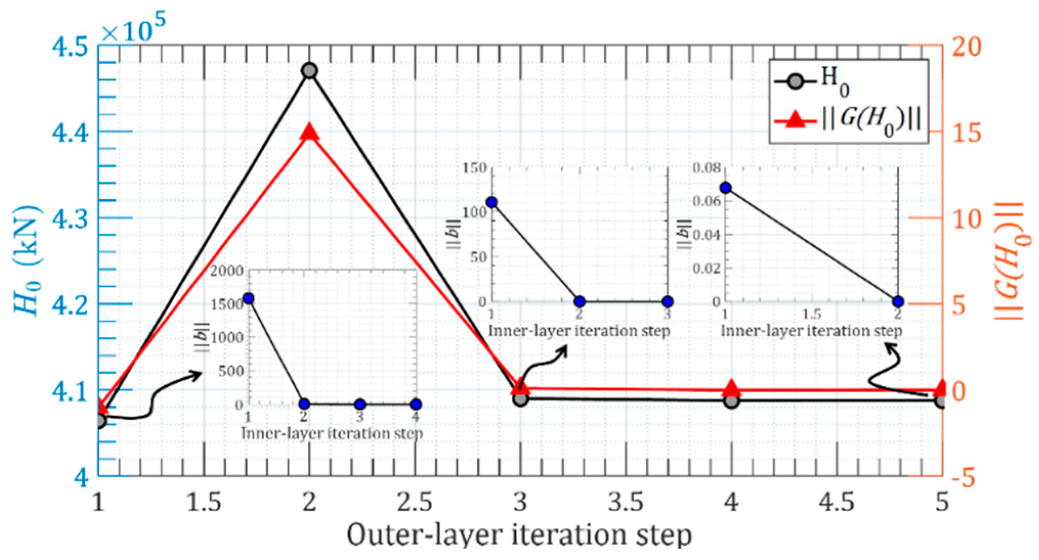
2.2. Nonlinear FEM Solution for the Cable Shape

A differential equation with the strong form is defined as $f\left(x,u,u^{\prime },u^{″},\cdots \right)=0$, in which $f(◾)$ is a function symbol, $x$ is the independent variable, $u$ is the dependent variable, $u^{\prime },u^{″},\cdots$ are the first-, second- and high-order derivatives with respect to the $x$. In FEM, it can be discretized using a basis function or a shape function $N_i$ to produce a weak form of ${{\displaystyle \int }}_{\mathsf{\Omega }}f\left(x,u,u^{\prime },u^{″},\cdots \right)N_{i}d\mathsf{\Omega }=0$, in which $\mathsf{\Omega }$ is the computational domain of interest. To solve the cable shape, a one-dimensional linear shape function is adopted in this study with the form of

$$N_i\left(x\right)=a_{i1}+a_{i2}x$$

(12)

in which $a_{i1}$ and $a_{i2}$ are undetermined coefficients estimated by the nodal coordinates of the element. By using the Galerkin’s method, the cable shape in terms of $y\left(x\right)$ and $z\left(x\right)$ can be formulated as:

$$y\left(x\right)=y_i{N}_i\left(x\right)$$

(13)

$$z\left(x\right)=z_i{N}_i\left(x\right)$$

(14)

By introducing the $N_i\left(x\right)$, the discrete algebraic form or weak form of Equations (9) and (10) can be expressed as:

$${{\displaystyle \int }}_0^L-H_0{y}^{″}{N}_i\left(x\right)dx+{{\displaystyle \int }}_0^{L}q\sqrt{1+{y^{\prime }}^2+{z^{\prime }}^2}{N}_i\left(x\right)dx+{{\displaystyle \int }}_0^L{T}_{yj}\delta \left(x-x_j\right)N_i\left(x\right)dx=0$$

(15)

$${{\displaystyle \int }}_0^L-H_0{z}^{″}{N}_i\left(x\right)dx+{{\displaystyle \int }}_0^L{T}_{zj}\delta \left(x-x_j\right)N_i\left(x\right)dx=0$$

(16)

in which the subscript $j$ (j = 1, 2, …, n) indicates the hanger ID, which is introduced to distinguish with the subscript $i$ before the Einstein summation convention is applied. The subscripts k and l in the following sections are also utilized for the same purpose. The integration by parts is applied to Equations (15) and (16), which leads to

$${{\displaystyle \int }}_0^L{H}_0{y}^{\prime }\frac{d{N}_i\left(x\right)}{dx}dx-H_0{y}^{\prime }{N}_i\left(x\right){|}_{\mathrm{BC}}+{{\displaystyle \int }}_0^{L}q\sqrt{1+{y^{\prime }}^2+{z^{\prime }}^2}{N}_i\left(x\right)dx+T_{yi}=0$$

(17)

$${{\displaystyle \int }}_0^L{H}_0{z}^{\prime }\frac{d{N}_i\left(x\right)}{dx}dx-H_0{z}^{\prime }{N}_i\left(x\right){|}_{\mathrm{BC}}+T_{zi}=0$$

(18)

in which BC indicates the integral boundary condition. The substitution of Equation (8) into Equations (17) and (18) produces:

$${{\displaystyle \int }}_0^L{H}_0{y}_j\frac{d{N}_j\left(x\right)}{dx}\frac{d{N}_i\left(x\right)}{dx}dx-H_0{y}^{\prime }{N}_i\left(x\right){|}_{\mathrm{BC}}+{{\displaystyle \int }}_0^{L}q\sqrt{1+{\left[y_j\frac{d{N}_j\left(x\right)}{dx}\right]}^2+{\left[z_j\frac{d{N}_j\left(x\right)}{dx}\right]}^2}{N}_i\left(x\right)dx+T_{yi}=0$$

(19)

$${{\displaystyle \int }}_0^L{H}_0{z}_j\frac{d{N}_j\left(x\right)}{dx}\frac{d{N}_i\left(x\right)}{dx}dx-H_0{z}^{\prime }{N}_i\left(x\right){|}_{\mathrm{BC}}+T_{zi}=0$$

(20)

in which $y_j$ and $z_j$ are the final y-direction and z-direction coordinates of the main cable. An additional formula for describing the ratio between $T_{yi}$ and $T_{zi}$ is given as:

$$\frac{T_{zi}}{T_{yi}}=\frac{z_i-z_{di}}{y_i-y_{di}}$$

(21)

As formulated in Equation (12), the differential of a one-dimensional linear shape function with respect to x is a constant for an element. Meanwhile, the node of the main cable that is located at the top of the pylon is assumed to be fixed. The Dirichlet boundary condition is therefore applied to the variables of y and z. The integral form of Equations (19) and (20) can be alternatively solved using a form of the summation as:

$${{\displaystyle \sum }}_{{\mathsf{\Omega }}_e}\left(H_0{y}_j\frac{d{N}_j\left(x\right)}{dx}\frac{d{N}_i\left(x\right)}{dx}dL\right)+{{\displaystyle \sum }}_{{\mathsf{\Omega }}_e}\left(q\sqrt{1+{\left[y_j\frac{d{N}_j\left(x\right)}{dx}\right]}^2+{\left[z_j\frac{d{N}_j\left(x\right)}{dx}\right]}^2}{{\displaystyle \int }}_0^L{N}_i\left(x\right)dx\right)+T_{yi}=0$$

(22)

$${{\displaystyle \sum }}_{{\mathsf{\Omega }}_e}\left(H_0{z}_j\frac{d{N}_j\left(x\right)}{dx}\frac{d{N}_i\left(x\right)}{dx}dL\right)+T_{yi}\frac{z_i-z_{di}}{y_i-y_{di}}=0$$

(23)

in which dL is the length of element ${\mathsf{\Omega }}_e$ in the x-direction. It is worth mentioning that ${\left[y_j\frac{d{N}_j\left(x\right)}{dx}\right]}^2$ and ${\left[z_j\frac{d{N}_j\left(x\right)}{dx}\right]}^2$ are constant within each element. However, their values are not identical for different elements. To solve this nonlinear equation related to $y_j$ and $z_j$, the Newton iteration method [33] is introduced:

$$x_{n+1}=x_n-\omega \frac{f\left(x_n\right)}{f^{\prime }\left(x_n\right)}$$

(24)

in which $f\left(x\right)$ is the function to be solved, $x_{n+1}$ is the approximate solution of $f\left(x\right)=0$ at (n + 1)-step iteration, $\omega$ is a relaxation coefficient, which is set as 1.0 in this study. $f^{\prime }\left(x_n\right)$ in Equations (22) and (23) is a matrix for a multivariable problem, which consists of the partial derivatives of the objective function with respect to each unknow variables:

$$K_{ij}^{yy}=\frac{\partial f_{yi}}{\partial y_j}={{\displaystyle \sum }}_{{\mathsf{\Omega }}_e}\left(H_0\frac{d{N}_j\left(x\right)}{dx}\frac{d{N}_i\left(x\right)}{dx}dL\right)+{{\displaystyle \sum }}_{{\mathsf{\Omega }}_e}\left(\frac{y_l\frac{d{N}_l\left(x\right)}{dx}\frac{d{N}_j\left(x\right)}{dx}{J}_i}{\sqrt{1+{(y_k\frac{d{N}_k\left(x\right)}{dx})}^2+{(z_k\frac{d{N}_k\left(x\right)}{dx})}^2}}\right)$$

(25)

$$K_{ij}^{yz}=\frac{\partial f_{yi}}{\partial z_j}={{\displaystyle \sum }}_{{\mathsf{\Omega }}_e}\left(\frac{z_l\frac{d{N}_l\left(x\right)}{dx}\frac{d{N}_j\left(x\right)}{dx}{J}_i}{\sqrt{1+{(y_k\frac{d{N}_k\left(x\right)}{dx})}^2+{(z_k\frac{d{N}_k\left(x\right)}{dx})}^2}}\right)$$

(26)

$$K_{ij}^{zy}=\frac{\partial f_{zi}}{\partial y_j}=\{\begin{array}{c}{T}_{yi}\frac{z_i-z_{di}}{{(y_i-y_{di})}^2}\\ 0\end{array} \begin{array}{c},i=j\\ ,i\ne j\end{array}$$

(27)

$$K_{ij}^{zz}=\frac{\partial f_{zi}}{\partial z_j}={{\displaystyle \sum }}_{{\mathsf{\Omega }}_e}\left(H_0\frac{d{N}_j\left(x\right)}{dx}\frac{d{N}_i\left(x\right)}{dx}dL\right)+\{\begin{array}{c}{T}_{yi}\frac{z_i}{y_i-y_{di}}\\ 0\end{array} \begin{array}{c},i=j\\ ,i\ne j\end{array}$$

(28)

in which $f_{yi}$ and $f_{zi}$ are functions described by the first members of Equations (22) and (23), which are derived from the equilibrium equations in y-direction Equation (9) and z-direction Equation (10) at ith point, respectively, $J_i={{\displaystyle \int }}_0^L{N}_i\left(x\right)dx=dL/2$ for the chosen one-dimensional linear shape function. To construct the Newton iteration form Equations (22) and (23) for the main cable, a matrix related to the $f^{\prime }\left(x_n\right)$ and a vector related to the $f\left(x_n\right)$ are assembled as:

$$\mathbf{K}=\left[\begin{array}{cc}{\mathit{K}}^{yy}& {\mathit{K}}^{yz}\\ {\mathit{K}}^{zy}& {\mathit{K}}^{zz}\end{array}\right]$$

(29)

$$\mathit{b}=\left(\begin{array}{c}{\mathit{f}}_y\\ {\mathit{f}}_z\end{array}\right)$$

(30)

in which ${\mathit{K}}^{yy}$, ${\mathit{K}}^{yz}$, ${\mathit{K}}^{zy}$, ${\mathit{K}}^{zz}$, ${\mathit{f}}_y$ and ${\mathit{f}}_z$ are obtained by assembling the $K_{ij}^{yy}$, $K_{ij}^{yz}$, $K_{ij}^{yz}$, $K_{ij}^{zz}$, $f_{yi}$ and $f_{zi}$ for all elements, ${\mathit{K}}^{yy}$, ${\mathit{K}}^{yz}$, ${\mathit{K}}^{zy}$ and ${\mathit{K}}^{zz}$ are matrices with the size of $n\times n$, ${\mathit{f}}_y$ and ${\mathit{f}}_z$ are matrices with the size of $n\times 1$. To solve the deformation increments of the main cable in y- and z-directions, i.e., $\Delta ={\left(dy dz\right)}^{\mathrm{T}}$, a linear algebra equation is then developed with the form of

$$\mathbf{K}\Delta =-\omega \mathit{b}$$

(31)

The nodal coordinates of the main cable are readily updated using the summation of the $\left(y_i z_i\right)$ and $\left(d{y}_i d{z}_i\right)$. It is worth noting that he initial nodal coordinates $\left(y_i,z_i\right)$ before the iteration can be assigned as arbitrary values, the coordinates of the intersection point (IP) between the pylon and main cable are suggested for the operational convenience. The above iteration scheme is illustrated in Figure 2 with a given $H_0$, which is called the inner-layer iteration in this study.

However, in most cases, $H_0$ is an undetermined parameter. The middle span-sag $f$ or the coordinate of the middle point in y-direction $y_{mid}$ of the main cable is always prescribed. An outer-layer iteration is therefore implemented, as described in Figure 2. At each outer-layer iteration, the coordinate of the middle point in y-direction ${\widehat{y}}_{mid}$ can be solved by a given $H_0$ using the inner-layer iteration. A one-to-one mapping relationship ${\widehat{y}}_{mid}=g\left(H_0\right)$ is assumed, in which $g(◾)$ is the function symbol. As a result, the solution of $H_0$ can be determined by finding the root of the equation $G\left(H_0\right)=g\left(H_0\right)-y_{mid}=0$. Since $g\left(H_0\right)$ has no explicit expression, the Secant method is utilized to achieve a numerical solution of $H_0$. The initial conditions for $H_1$ and $H_2$ are suggested as the 1.0 time and 1.1 times of

$$H_0=\frac{L{{\displaystyle \sum }}_{i=1}^n{T}_{yi}}{8f}$$

(32)

For two-dimensional parallel main cables, the coordinate of a main cable in z-direction $z_i$ is an invariant constant. The $\mathbf{K}$ can reduced to a $n\times n$ matrix as $\mathbf{K}=K^{yy}$, in which $K^{yy}$ is assembled from the $K_{ij}^{yy}$ by removing the $z_i$-related terms in Equation (25) with the form of

$$K_{ij}^{yy}=\frac{\partial f_{yi}}{\partial y_j}={{\displaystyle \sum }}_{{\mathsf{\Omega }}_e}\left(H_0\frac{d{N}_j\left(x\right)}{dx}\frac{d{N}_i\left(x\right)}{dx}dL\right)+{{\displaystyle \sum }}_{{\mathsf{\Omega }}_e}\left(\frac{y_l\frac{d{N}_l\left(x\right)}{dx}\frac{d{N}_j\left(x\right)}{dx}{J}_i}{\sqrt{1+{(y_k\frac{d{N}_k\left(x\right)}{dx})}^2}}\right)$$

(33)

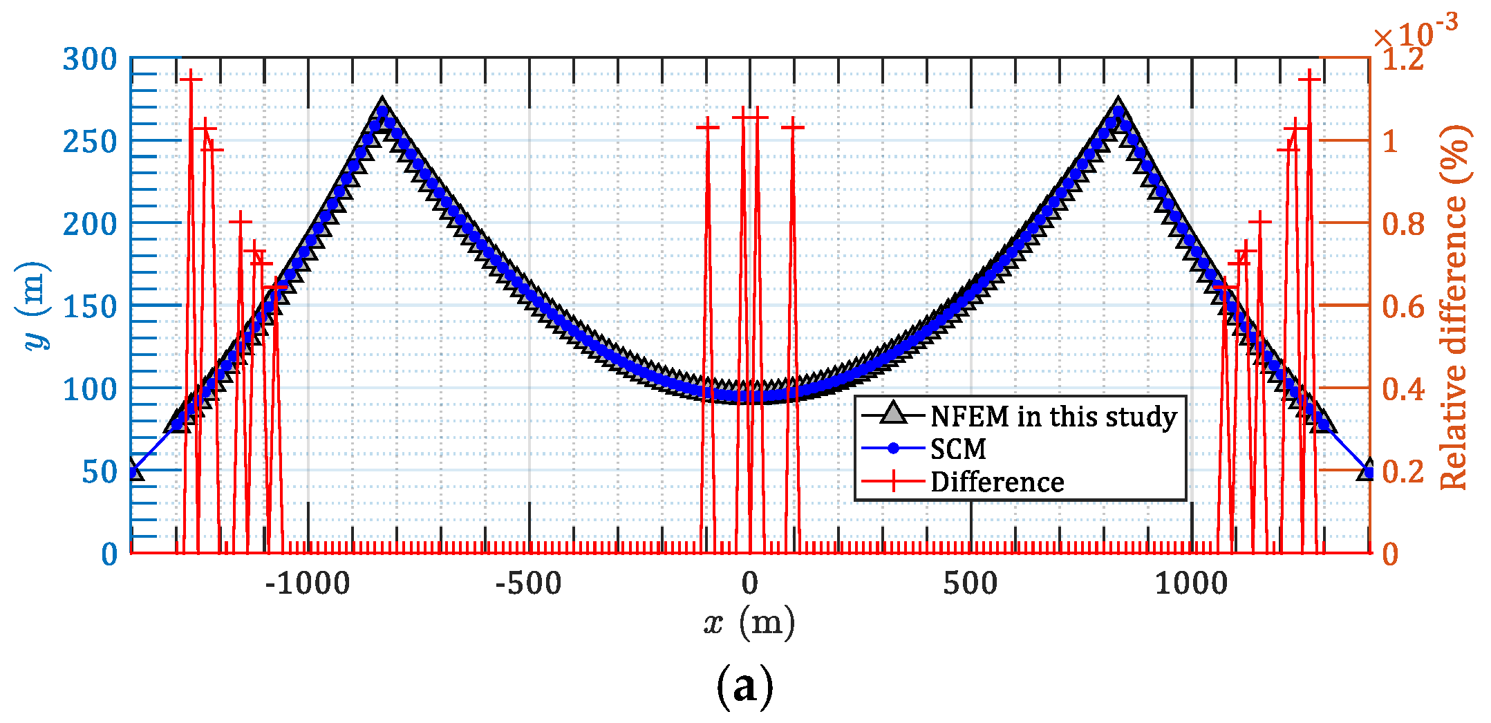
2.3. Comparison with the Segmental Catenary Method

The segmental catenary method is an exact solution for an element of the main cable deformed due to its self-weight. The lengths of each segment in x- y- and z-directions are solved as:

$$l_x=\frac{F_x}{E_c{A}_c}{l}_0-\frac{F_x}{q}\left\{{\sin \mathrm{h}}^{-1}\left(\frac{F_y}{H_0}\right)-{\sin \mathrm{h}}^{-1}\left(\frac{F_y-q{l}_0}{H_0}\right)\right\}$$

(34)

$$l_y=\frac{F_z}{E_c{A}_c}{l}_0-\frac{F_z}{q}\left\{{\sin \mathrm{h}}^{-1}\left(\frac{F_y}{H_0}\right)-{\sin \mathrm{h}}^{-1}\left(\frac{F_y-q{l}_0}{H_0}\right)\right\}$$

(35)

$$l_z=\frac{F_y}{E_c{A}_c}{l}_0-\frac{F_x}{2E_c{A}_c}-\frac{H_0}{q}\left[\sqrt{1+{\left(\frac{F_y}{H_0}\right)}^2}-\sqrt{1+{\left(\frac{F_y-q{l}_0}{H_0}\right)}^2}\right]$$

(36)

in which $l_x$, $l_y$ and $l_z$ are the distances between the two nodes of a segment along the global x- y- and z-axes, $F_x$, $F_y$ and $F_z$ are three components of the global nodal force, $E_c$ is the elastic modulus of the main cable, $A_c$ is the cross-sectional area, $q$ is the self-weight of the main cable per unit length, $l_0$ is the unstrained length of the cable segment. Figure 3 illustrates the iteration scheme of the segmental catenary method. For a two-pylon suspension bridge, a guess of the axial force ${\mathit{F}}_1=\left(F_{x1},F_{y1},F_{z1}\right)$ at one end of the main cable is made first. The unstrained length $l_{01}$ and $l_{y1}$ and $l_{z1}$ of first segment are obtained by solving the transcendental equations described in Equations (34) and (36). The axial force of next segment, which will be used to solve the $l_{02}$ and $l_{y2}$ and $l_{z2}$ is then readily calculated by introducing the tensile force of the first hanger. ${\mathit{F}}_1$ will be adjusted by comparing the coordinates of the IP at the other pylon in y- and z-directions, i.e., $y_{IP}$ and $z_{IP}$ with the calculated ${\widehat{y}}_{IP}$ and ${\widehat{z}}_{IP}$ as well as the $y_{mid}$ with ${\widehat{y}}_{mid}$ to achieve a convergent solution.

A comparison between the SCM and present NFEM is shown in

Table 1. Comparison between the SCM and NFEM.

Method	Object	Coordinate System	Governing Equations	Axis Stiffness of Cable
entry 1	Cable segment	Lagrangian (with respect to l0)	Algebraic equations	Yes
entry 2	Whole cable	Eulerian (with respect to x)	Differential equations	No

. The SCM focuses on each cable segment to develop its analytical expression of the cable shape using algebraic equations (Equations (34) and (36)) in the Lagrangian coordinate system with respect the unstrained cable length $l_0$. The present NFEM solves the differential equations of the whole cable in the Eulerian coordinate system with respect the bridge axis coordinate x using the nonlinear finite element approximation. The SCM requires the inputs of the axis stiffness of the cable, i.e., $E_c{A}_c$ to determine the unstrained cable length while no information regarding the cable material or cross section is needed in the NFEM for solving the cable shape. It is noteworthy that the unstrained cable length, which is of great importance during the construction stage, can also be calculated using the NFEM by subtracting the elongation from the final length of the cable.

3. Cases Study

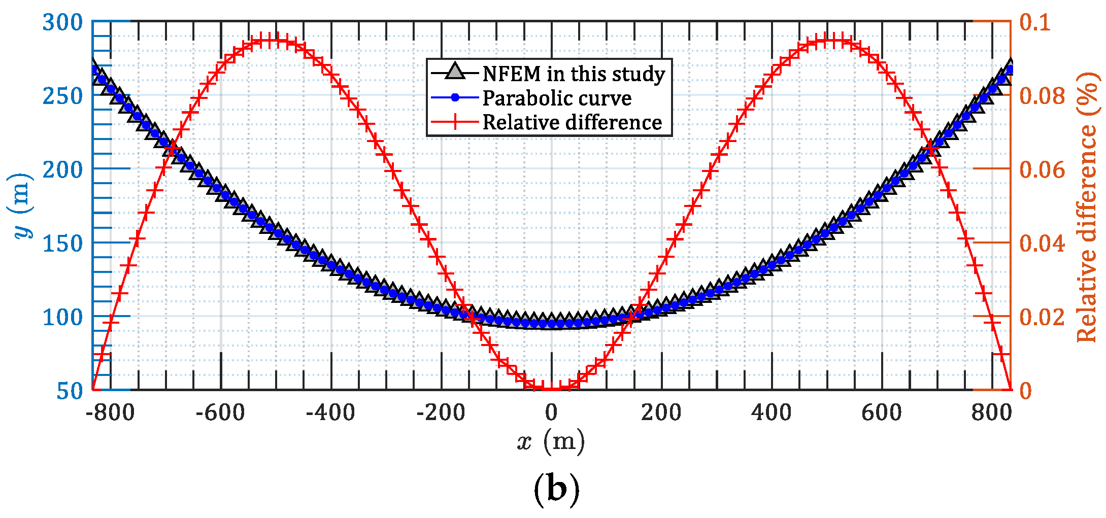
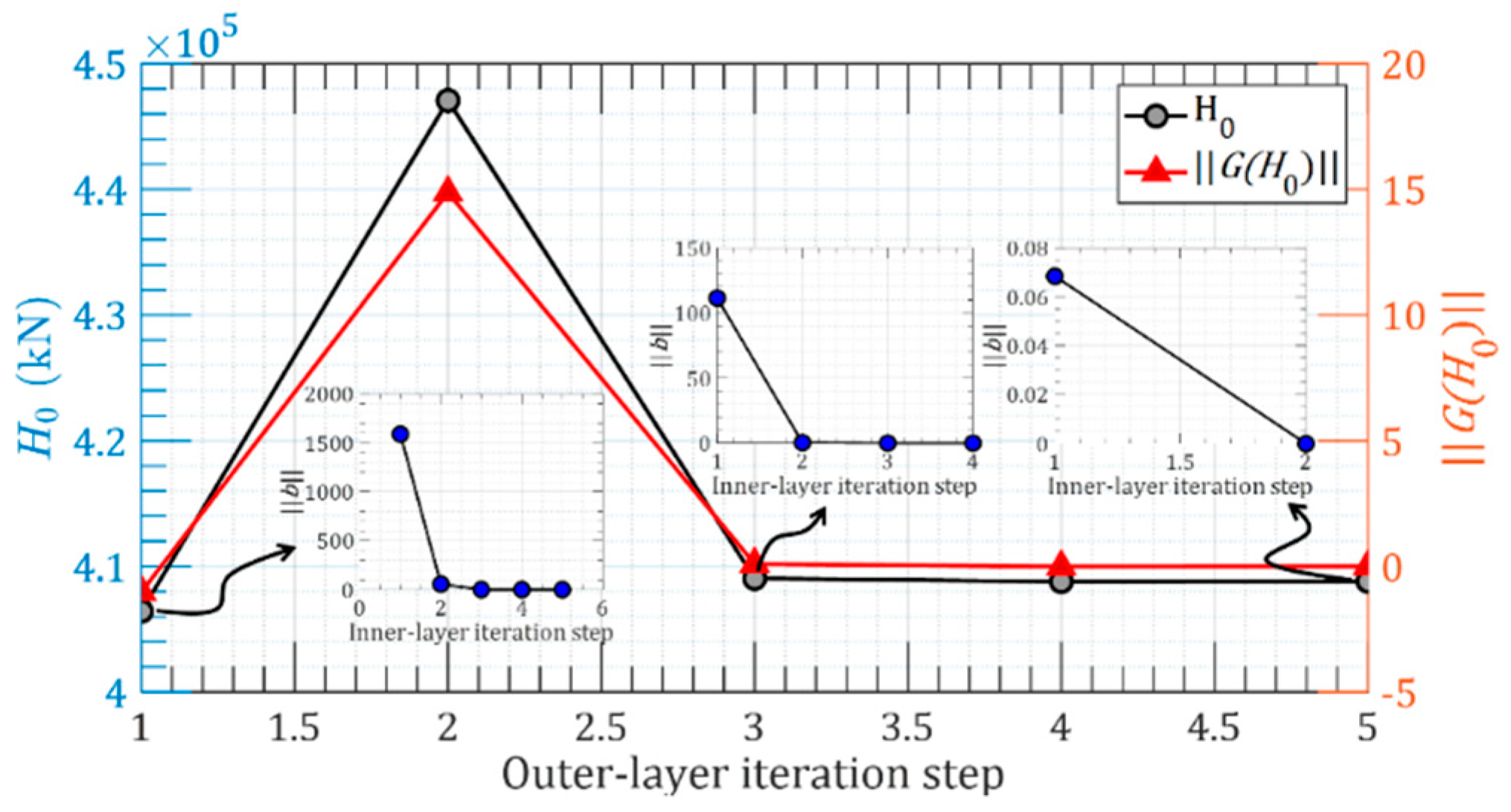
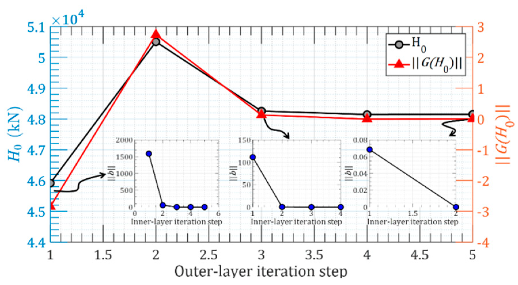
3.1. Case 1: 2D Parallel Main Cables of an Earth-Anchored Suspension Bridge

An earth-anchored suspension bridge with 2D parallel main cables is utilized, as shown in Figure 4. The main span is 1666 m, and the side span is 500 m with a sag of 172.64 m in the main span. The designed sag-span ratio is 9.65. A single box girder with the width of the 49.7 m is adopted. The height of the bridge tower is 265 m and the elevations of the two IP points at the tops of the pylons are 267.414 m. There are two parallel vertical cable planes, each of which consists of a main cable as well as 29 hangers in the side span and 103 hangers in the main span. The spacing between two parallel cables in z-direction is 41 m. The cable segment lengths in the x-direction are 35 m + 28 × 16 m + 17 m in the side span and 17 m + 102 × 16 m + 17 m in the main span. The cable self-weight per unit length $q=54.088$ kN/m. The elastic modulus and the cross area of the main cable are $E_c=1.96\mathrm{E}11\mathrm{N}/{\mathrm{m}}^2$ and $A_c=0.706{ \mathrm{m}}^2$. The origin of the Eulerian coordinate system is set at the midpoint of the bridge with zero elevation.

The nodal force or the tension of each hanger $T_{yi}$ in y-direction is estimated from the dead loads of the stiffening girder by introducing the boundary conditions of the girder. The displacements of the intersection point between the girder and pylon in y-direction are coupled. The intersection point between the girder and transition pier is coupled in y- and z-directions as well as the rotation degree of freedom with respect to the x-axis. The estimated hanger tension forces in y-direction are shown in Figure 5. The maximum value of 3781.2 kN occurs at the first hanger in the side span while the most hangers have the tension of 2372.5.2 kN. The sag is given as f = 172.64 m at the beginning, which indicates y_mid = 267.414 − 172.640 = 94.774 m.

Two-layer iterations are implemented to perform the shape finding process for the main cable by following the scheme in Figure 2. The outer-layer and inner-layer iteration tolerances are set as ${\epsilon }_1=1.0\times {10}^{-4}$ and ${\epsilon }_2=1.0\times {10}^{-6}$. Figure 6 illustrates the iteration results, in which a convergent horizontal component of the axial force, i.e., $H_0$ is achieved in five outer-layer iteration steps. Between each adjacent outer-layer iterations, less than four-step inner-layer iterations are required for solving the cable shape. The main cable shape from the initial input coordinates of to the final shape finding result that corresponds the final outer- and inner-layer iteration is plotted in Figure 7. The shape finding using the commonly used segment catenary method (SCM) is also conducted as a benchmark for comparison purpose. Both the final main cable shapes obtained from this study and the SCM are given in Figure 8a, showing a reasonable agreement with each other. The maximum relative difference at all hanger nodes is 0.0011%. Moreover, the parabolic curve of the main cable in the middle span calculated by the $y=y_{IP}+4f\left(x^2-L^2/4\right)/L^2$ is also compared with the present solution, as shown in Figure 8b. The difference between these two methods is also insignificant with the maximum relative error of 0.0948%. This is mainly because of the sag-span ratio of this suspension bridge about equal to 1/10 such that the dead loadings along the along the bridge approximately follow the uniform distribution. Furthermore, the static displacement of the final main cable under the action of self-weight and hanger tension forces is analyzed using the FEM, as shown in Figure 9. As can be seen, all nodal displacements of the main cable are less than 0.007 m. It is sufficiently small to believe that the main cable has achieved the target configuration. It is noteworthy that the time costs in this case for both the NFEM and the SCM are less than one second.

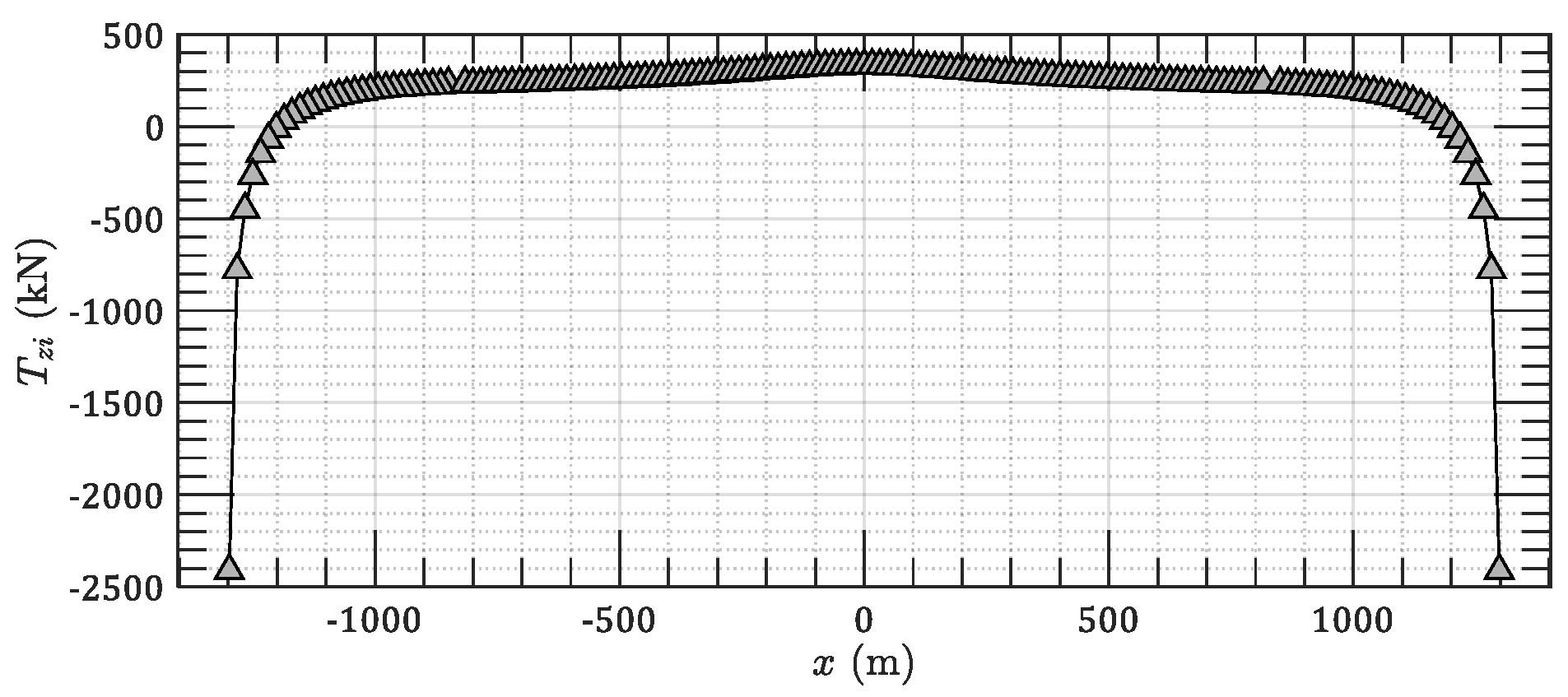
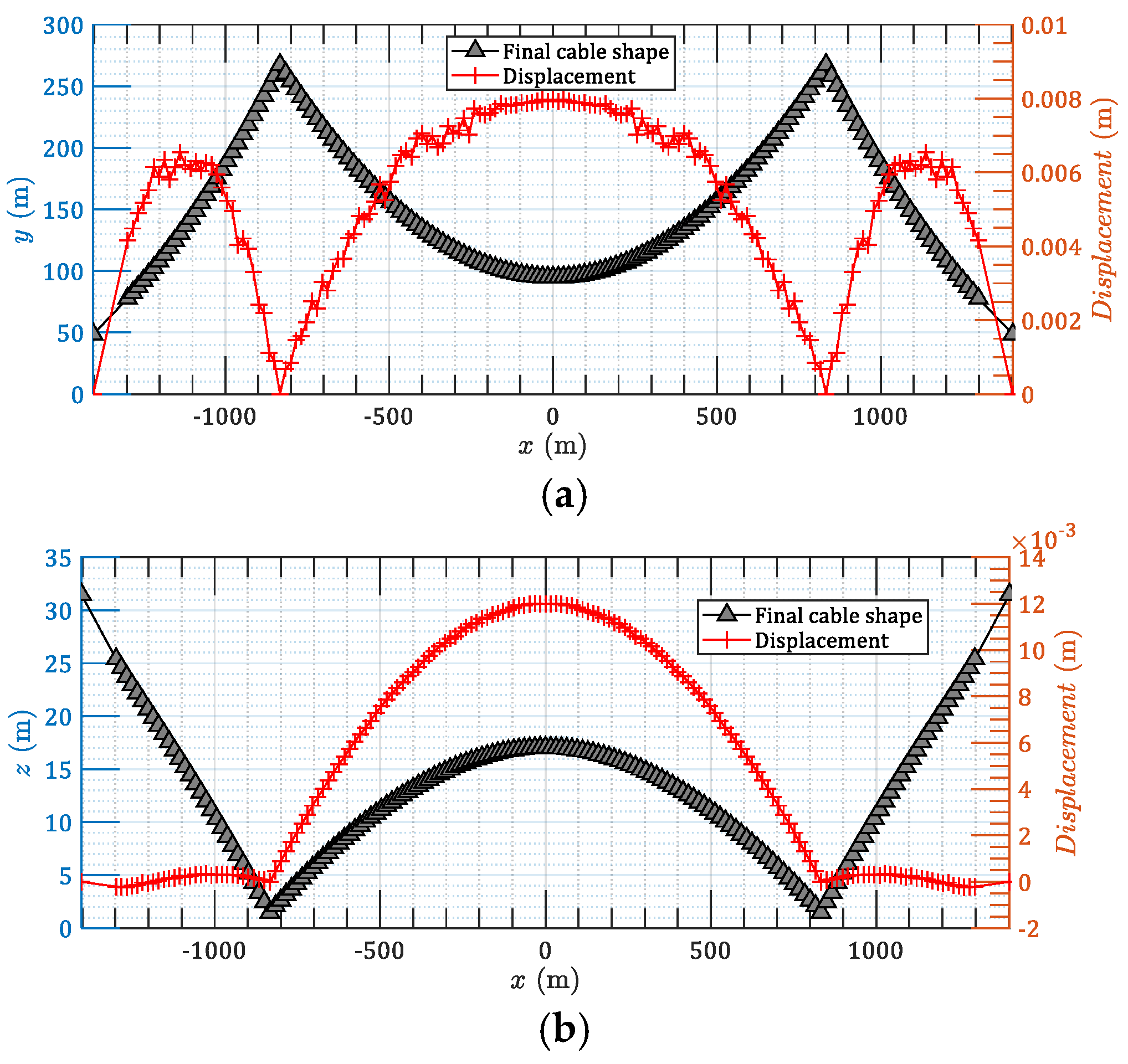
3.2. Case 2: 3D Spatial Main Cables of an Earth-Anchored Suspension Bridge

Three dimensional spatial main cables are applied to the same suspension bridge used in Case 1. The spacings between two cables at the position of the anchorage and the IP points in z-direction are set as 63.0 m and 3.0 m, respectively, as shown in Figure 10. The vertical (y-direction) force components of all hangers given in Figure 5 are identical to Case 1. Same tolerances are also employed in this case, say ${\epsilon }_1=1.0\times {10}^{-4}$ and ${\epsilon }_2=1.0\times {10}^{-6}$. The iteration process is shown in Figure 11. Similar to the Case 1, five outer-layer iterations are implemented to obtain a convergent $H_0$. All inner-layer iterations are less than five steps to meet the tolerance requirement. The main cable shape from the initial input coordinates in y- and z-directions to the final target configurations is illustrated in Figure 12. The final shape of the 2D parallel main cables in Case 1 is also plotted in Figure 12a. As can be seen, the shapes in y-direction of 2D planar cable and 3D spatial cable match well with each other. This can be explained by comparing the governing equations for the cable shape described by Equations (9) and (11). The difference of the cable shapes in x-o-y plane for parallel and spatial cases in mainly attributed to the $z^{\prime }$. For the long-span suspension bridge studied in this case, the slope in z-direction of the spatial cable is small as compared to the slope in y-direction, resulting in that the effect of the ${z^{\prime }}^2$ in Equations (9) and (10) is insignificant. This can also be demonstrated from the final main shape in Figure 12. The calculated maximum ${y^{\prime }}^2$ and ${z^{\prime }}^2$ using the central difference method are 0.2593 and 0.0033, respectively.

Figure 13 illustrates the solution of hanger tension components in z-direction along the bridge span. The positive tension indicates that the inclination of the hanger tilts inward. The maximum positive tension in z-direction occurs at the middle span with the value of 331.637 kN. The negative tensions for outward inclined hangers at two side spans reach the maximum for first or end hanger. This is because the vertical component of the tension for first or end hanger as shown in Figure 5 is large. Figure 14 compares the cable shape between this study and the results obtained by SCM. The maximum relative differences at all hanger nodes in y- and z-direction are 0.0022% and 0.7318%, respectively, suggesting a reasonable agreement with each other. To further validate the accuracy of the final cable shape, a finite element model of the spatial main cable is also established. The static displacement under the action of self-weight and hanger tension forces is illustrated in Figure 15. It can be found that the maximum displacements in y- and z-direction of the main cable are 0.008 m and 0.012 m, which are sufficiently small and acceptable for the engineering applications.

3.3. Case 3: 3D Spatial Main Cables of a Self-Anchored Suspension Bridge

Another case is the Yongjong Grand Bridge in Korea, whose shape finding was investigated by many pioneering studies [16,22,26]. The Yongjong Grand Bridge is the first highway and railway self-anchored suspension bridge with three dimensional main cables. The total length of the bridge is 550 m with a 300-m main span and two 125-m side spans. The sag in middle span is 60 m. $T_{yi}$ has a uniform value of 3.048 KN. The cross-sectional area of the main cable is 0.1355 m². The y and z coordinate values of the IP point are $y_{IP}=114.573 \mathrm{m}$ and $z_{IP}=1.50 \mathrm{m}$, respectively by setting the origin of the Eulerian coordinate system at the midpoint of the bridge with zero elevation. The main cable is divided into 24 segments by 23 hangers. The coordinates of the connection points between hangers and the beam, i.e., $y_{di}$ and $z_{di}$ are estimated from the data given by Kim et al. [16] and Luo et al. [26], as listed in

Table 2. Coordinate values of joint points for suspenders and girder.

x (m)	${\mathit{y}}_{\mathit{d}\mathit{i}}$ (m)	${\mathit{z}}_{\mathit{d}\mathit{i}}$ (m)
125.000	48.870	15.960
137.500	48.994	15.960
150.000	49.108	15.960
162.500	49.210	15.960
175.000	49.302	15.960
187.500	49.383	15.960
200.000	49.453	15.960
212.500	49.512	15.960
225.000	49.561	15.960
237.500	49.599	15.960
250.000	49.626	15.960
262.500	49.642	15.960
275.000	49.647	15.960

. The IP point is located at x = 125.0 m, and the mid-point of the main span is at x = 275 m.

The iteration process for the Yongjong Grand Bridge using present method is illustrated in Figure 16. Both the outer-layer and inner-layer iterations meet the tolerance requirement in five steps. The solved horizontal component of the cable axial force is 48,149.1 kN, which is close to the value, 49,541 kN given by Kim et al. [16] with the relative error of 2.89 %. The solution of the cable shape is compared with the results obtained by Kim et al. [16] and Luo et al. [26] in

Table 3. Comparison between the results in this study and other studies.

x(m)	Kim et al. (2002) (A)		Luo et al. (2004) (B)		This Study (C)		A vs. C (%)		B vs. C (%)
	y (m)	z (m)	y (m)	z (m)	y (m)	z (m)	(yA − yC)/yA	(zA − zC)/zA	(yB − yC)/yB	(zB − zC)/zB
125.000	114.573	1.500	113.763	1.681	114.573	1.500	-	-	-	-
137.500	104.938	3.632	104.968	3.625	104.927	3.644	0.010	−0.330	0.039	−0.524
150.000	96.160	5.586	96.180	5.576	96.141	5.605	0.020	−0.340	0.041	−0.520
162.500	88.230	7.360	88.243	7.350	88.208	7.382	0.025	−0.299	0.040	−0.435
175.000	81.147	8.955	81.155	8.944	81.125	8.976	0.027	−0.235	0.037	−0.358
187.500	74.905	10.369	74.910	10.357	74.885	10.386	0.027	−0.164	0.033	−0.280
200.000	69.502	11.601	69.505	11.590	69.485	11.612	0.024	−0.095	0.029	−0.190
212.500	64.935	12.650	64.937	12.639	64.923	12.654	0.018	−0.032	0.022	−0.119
225.000	61.201	13.514	61.203	13.504	61.194	13.510	0.011	0.030	0.015	−0.044
237.500	58.300	14.191	58.301	14.183	58.296	14.179	0.007	0.085	0.009	0.028
250.000	56.228	14.678	56.230	14.671	56.227	14.661	0.002	0.116	0.005	0.068
262.500	54.985	14.973	54.987	14.966	54.987	14.951	−0.004	0.147	0.000	0.100
275.000	54.573	15.071	54.573	15.065	54.573	15.049	0.000	0.146	0.000	0.106

. As can be seen, the relative differences in y-direction between the present study and Kim et al. [16] are less than 0.027%. In z-direction, the absolute values of the relative difference are less than 0.340%. The location of the IP was further studied by Luo et al. [26], which is different from the coordinates used in the present study and Kim et al. [16]. The maximum absolute value of the relative difference between present study and Luo et al. [26] in y and z directions are 0.041% and 0.524%, respectively, which are slightly larger than the errors between the present study and Kim et al. [16]. However, the present method is proved to be accurate enough to find a reasonable cable shape of the suspension bridge for engineering applications.

4. Conclusions

This paper develops a novel shape finding approach for main cable-only systems under specified loads. The governing differential equations for the main cable in Eulerian coordinate system are constructed. Two-layer numerical iterations are then conducted to solve the governing equations using the nonlinear finite element approximation. The proposed method is applied to three cases, i.e., 2D parallel and 3D spatial main cables of an earth-anchored suspension bridge as well as the 3D spatial main cables of a self-anchored suspension bridge to achieve the target configuration of the main cable. Comparisons with the SCM and other studies are also performed to validate the accuracy of the present method. Some conclusions can be summarized as follows:

(1)

The proposed shape finding technique enables an efficient and accurate estimation of the target configuration of the main cable for the suspension bridge.

(2)

The present NFEM performs the form-finding for the whole cable in the Eulerian coordinate system using a few iteration steps without any information of the cable material or cross area as compared with the commonly used SCM. The unstrained cable length can also be calculated by subtracting the elongation from the final length of the cable.

(3)

Both the SCM and the present NFEM methods have enough efficiency and accuracy for finding final cable shape of the suspension bridge. The proposed technique provides an alternative to be used by the bridge designers and engineers for the rapid estimation of both 2D parallel and 3D spatial cable curves in the preliminary design stage.

References

1. Xiang, H.F.; Ge, Y.J. Aerodynamic challenges in span length of suspension bridges. Front. Archit. Civ. Eng. China 2005, 1, 153–162. [Google Scholar] [CrossRef]
2. Atmaca, B.; Ates, S. Construction stage analysis of three-dimensional cable-stayed bridges. Steel. Compos. Struct. 2012, 5, 413–426. [Google Scholar] [CrossRef]
3. Zhang, W.M.; Li, T.; Shi, L.Y.; Liu, Z.; Qian, K.R. An iterative calculation method for hanger tensions and the cable shape of a suspension bridge based on the catenary theory and finite element method. Adv. Struct. Eng. 2019, 22, 1566–1578. [Google Scholar] [CrossRef]
4. Gimsing, N.J.; Georgakis, C.T. Cable Supported Bridges; John Wiley & Sons, Ltd.: Hoboken, NJ, USA, 2012; Volume 3. [Google Scholar]
5. Wu, Z.Q.; Wei, J. Nonlinear Analysis of Spatial Cable of Long-Span Cable-Stayed Bridge considering Rigid Connection. KSCE J. Civ. Eng. 2019, 23, 148–215. [Google Scholar] [CrossRef]
6. Yuan, X.; Dong, S. A two-node curved cable element for nonlinear analysis. Eng. Mech. 1999, 4, 007. (In Chinese) [Google Scholar]
7. Yang, M.; Chen, Z. Nonlinear analysis of cable structures using a two-node curved cable element of high precision. Eng. Mech. 2003, 20, 42–47. (In Chinese) [Google Scholar]
8. Kwan, A. A new approach to geometric nonlinearity of cable structures. Comput. Struct. 1998, 67, 243–252. [Google Scholar] [CrossRef]
9. Ever, C.; Leonardo, F. Nonlinear analysis of structures cable-truss. Int. J. Eng. Technol. Sci. 2015, 7, 160–169. [Google Scholar]
10. Ahmad, A.M.S.; Ahmad, S.; Vahab, E.; Alireza, N.R. Nonlinear analysis of cable structures under general loadings. Finite Elem. Anal. Des. 2013, 73, 11–19. [Google Scholar]
11. Andreu, A.; Gil, L.; Roca, P. A new deformable catenary element for the analysis of cable net structures. Comput. Struct. 2006, 84, 1882–1890. [Google Scholar] [CrossRef]
12. Li, C.X.; He, J.; Zhang, Z.; Liu, Y.; Ke, H.J.; Dong, C.W.; Li, H. An Improved Analytical Algorithm on Main Cable System of Suspension Bridge. Appl. Sci. 2018, 8, 1358. [Google Scholar] [CrossRef] [Green Version]
13. Chen, Z.; Cao, H.; Zhu, H.; Hu, J.; Li, S. A simplified structural mechanics model for cable-truss footbridges and its implications for preliminary design. Eng. Struct. 2014, 68, 121–133. [Google Scholar] [CrossRef]
14. Irvine, H.M. Cable Structures; MIT Press: Cambridge, MA, USA, 1981. [Google Scholar]
15. Xiao, R.C.; Xiang, H.F. Research on method and program system for determining ideal state of suspension bridge with large span. East China Highw. 1998, 11, 42–50. (In Chinese) [Google Scholar]
16. Kim, H.K.; Lee, M.J.; Chang, S.P. Non-linear shape-finding analysis of a self-anchored suspension bridge. Eng. Struct. 2002, 24, 1547–1559. [Google Scholar] [CrossRef]
17. Tang, M.L. Spatial Geometric Nonlinear Analysis and Software Development of Long Span Suspension Bridges. Ph.D. Thesis, Southwest Jiaotong University, Chengdu, China, 2003. (In Chinese). [Google Scholar]
18. Zhang, W.M.; Yang, C.Y.; Wang, Z.W.; Liu, Z. An analytical algorithm for reasonable central tower stiffness in the three-tower suspension bridge with unequal-length main spans. Eng. Struct. 2019, 199, 109595. [Google Scholar] [CrossRef]
19. Kim, K.S.; Lee, H.S. Analysis of target configurations under dead loads for cable-supported bridges. Comput. Struct. 2001, 79, 2681–2692. [Google Scholar] [CrossRef]
20. Kim, M.Y.; Kim, D.Y.; Jung, M.R.; Attard, M.M. Improved methods for determining the 3-dimensional initial shapes of cable-supported bridges. Int. J. Steel. Struct. 2014, 14, 83–102. [Google Scholar] [CrossRef]
21. Kim, M.Y.; Jung, M.R.; Attard, M.M. Unstrained length-based methods determining an optimized initial shape of 3-dimensional self-anchored suspension bridges. Comput. Struct. 2019, 217, 18–35. [Google Scholar] [CrossRef]
22. Sun, Y.; Zhu, H.P.; Dong, X. New method for shape finding of self-anchored suspension bridges with three-dimensionally curved cables. J. Bridge Eng. 2015, 20, 04014063. [Google Scholar] [CrossRef]
23. Luongo, A.; Zulli, D. Static perturbation analysis of inclined shallow elastic cables under general 3D-loads. Curved. Layer. Struct. 2016, 5, 250–259. [Google Scholar] [CrossRef]
24. Luongo, A.; Zulli, D. Statics of shallow inclined elastic cables under general vertical loads: A perturbation approach. Mathematics 2018, 6, 24. [Google Scholar] [CrossRef] [Green Version]
25. Tang, M.L.; Qiang, S.Z.; Shen, R.Z. Segmental catenary method of calculating the cable curve of suspension bridge. J. China Railw. Soc. 2003, 25, 87–91. (In Chinese) [Google Scholar]
26. Luo, X.H.; Xiao, R.C.; Xiang, H.F. Cable shape analysis of suspension bridge with spatial cables. J. Tongji Univ. 2004, 32, 1349–1354. (In Chinese) [Google Scholar]
27. Wang, S.R.; Zhou, Z.X.; Huang, Y.Y.; Gao, Y.M. Analytical calculation method for the preliminary analysis of self-anchored suspension bridges. Math. Probl. Eng. 2015, 3, 1–12. [Google Scholar] [CrossRef] [Green Version]
28. Zhou, Y.F.; Chen, S. Iterative Nonlinear Cable Shape and Force Finding Technique of Suspension Bridges Using Elastic Catenary Configuration. J. Eng. Mech. 2019, 145. [Google Scholar] [CrossRef]
29. Li, T.; Liu, Z. A Recursive Algorithm for Determining the Profile of the Spatial Self-anchored Suspension Bridges. KSCE J. Civ. Eng. 2019, 23, 1283–1292. [Google Scholar] [CrossRef]
30. Xiao, R.C.; Chen, M.H.; Sun, B. Determination of the reasonable state of suspension bridges with spatial cables. J. Bridge Eng. 2017, 22, 04017060. [Google Scholar] [CrossRef]
31. Song, C.L.; Xiao, R.C.; Sun, B. Improved Method for Shape Finding of Long-Span Suspension Bridges. Int. J. Steel Struct. 2020, 20, 247–258. [Google Scholar] [CrossRef]
32. Zienkiewicz, O.C.; Taylor, R.L. The Finite Element Method; McGraw-Hill: London, UK, 1967; Volume 3. [Google Scholar]
33. Cheney, E.; Kincaid, D. Numerical Mathematics and Computing; Nelson Education: Toronto, ON, Canada, 2012. [Google Scholar]
Figure 1. The coordinate system and loading distribution of the spatial main cable: (a) Three-dimensional coordinate; (b) Two-dimensional coordinate of the cross section.
Applsci 11 04644 g001
Figure 2. Flowchart of the iteration scheme for solving the cable shape.
Applsci 11 04644 g002
Figure 3. Flowchart of the iteration scheme for solving the cable shape of segmental catenary method.
Applsci 11 04644 g003
Figure 4. Layout of the suspension bridge using parallel main cables.
Applsci 11 04644 g004
Figure 5. Hanger tension forces in y-direction along the bridge span.
Applsci 11 04644 g005
Figure 6. Outer-layer and inner-layer iteration results for 2D parallel main cables.
Applsci 11 04644 g006
Figure 7. The cable shape from the initial coordinates to the target configuration for 2D parallel main cables.
Applsci 11 04644 g007
Figure 8. Comparison of the cable shape for 2D parallel main cable: (a) NFEM vs. SCM; (b) NFEM vs. Parabolic theory.
Applsci 11 04644 g008aApplsci 11 04644 g008b
Figure 9. Static displacement of the final 2D parallel main cable achieved by the FEM.
Applsci 11 04644 g009
Figure 10. Top view of the suspension bridge using spatial main cables (A half of the bridge).
Applsci 11 04644 g010
Figure 11. Outer-layer and inner-layer iteration results for 3D spatial main cables in Case 2.
Applsci 11 04644 g011
Figure 12. The main cable shape from the initial coordinates to the target configuration for 3D spatial main cables: (a) y-direction; (b) z-direction.
Applsci 11 04644 g012
Figure 13. Hanger tension components in z-direction along the bridge span.
Applsci 11 04644 g013
Figure 14. Comparison of the cable shape obtained from the NFEM and SCM for 3D spatial main cables: (a) y-direction; (b) z-direction.
Applsci 11 04644 g014
Figure 15. Static displacement of the final 3D spatial main cable achieved by the FEM: (a) y-direction; (b) z-direction.
Applsci 11 04644 g015
Figure 16. Outer-layer and inner-layer iteration results for 3D spatial main cables in Case 3.
Applsci 11 04644 g016