Abstract
In the domain of functional magnetic resonance imaging (fMRI) data analysis, given two correlation matrices between regions of interest (ROIs) for the same subject, it is important to reveal relatively large differences to ensure accurate interpretation. However, clustering results based only on differences tend to be unsatisfactory and interpreting the features tends to be difficult because the differences likely suffer from noise. Therefore, to overcome these problems, we propose a new approach for dimensional reduction clustering. Methods: Our proposed dimensional reduction clustering approach consists of low-rank approximation and a clustering algorithm. The low-rank matrix, which reflects the difference, is estimated from the inner product of the difference matrix, not only from the difference. In addition, the low-rank matrix is calculated based on the majorize–minimization (MM) algorithm such that the difference is bounded within the range to 1. For the clustering process, ordinal k-means is applied to the estimated low-rank matrix, which emphasizes the clustering structure. Results: Numerical simulations show that, compared with other approaches that are based only on differences, the proposed method provides superior performance in recovering the true clustering structure. Moreover, as demonstrated through a real-data example of brain activity measured via fMRI during the performance of a working memory task, the proposed method can visually provide interpretable community structures consisting of well-known brain functional networks, which can be associated with the human working memory system. Conclusions: The proposed dimensional reduction clustering approach is a very useful tool for revealing and interpreting the differences between correlation matrices, even when the true differences tend to be relatively small.
1. Introduction
Currently, the neural basis of the human cognitive system is studied using noninvasive neuroimaging techniques such as functional magnetic resonance imaging (fMRI), electroencephalography (EEG), and functional near-infrared spectroscopy (fNIRS) [1,2,3,4]. In particular, for investigating the complex and distinctive functional network structure of the human brain and its nervous system [5,6], functional connectivity analysis, which examines the temporal synchronization between brain regions (e.g., [7]), is gaining popularity in this field. Functional connectivity between specific regions of interest (ROIs) is usually compared among various subjects or experimental conditions. Additionally, the patterns of functional connections are often analyzed in terms of network structures, such as community structure and network centrality. For example, recent studies have revealed that the community structures of functional connectivity networks differ not only between schizophrenic individuals and healthy controls [8] but also during the performance of different cognitive tasks [9].
Here, we focus on situations in which correlation matrices between ROIs are calculated for each subject in two different conditions. In such situations, it is important to reveal subnetworks of ROIs such that the differences between conditions are relatively large. However, it is difficult to interpret the features of distinctive clusters because the range of correlations is bounded, i.e., , and the differences are affected by observational error.
In [10], through the use of benchmark data sets, it was reported that increasing the number of dimensions does not affect the clustering results. On the other hand, in [11], it was demonstrated that clustering results tend to be worse when the data include noise, irrespective of the clustering method used, such as k-means. Concretely, we assume a situation such that some meaningful variables include a clustering structure, e.g., [12], whereas the other variables do not and are considered as noise. In this situation, it is difficult to detect the clustering structure using a clustering algorithm. One very useful approach for addressing this problem is low-rank approximation for the difference matrix. Here, dimensional reduction signifies estimating a low-rank correlation matrix from the full-rank difference matrix; that is, the estimated low-rank approximation can emphasize the clustering structure. However, such estimated low-rank matrices occasionally lose clustering structure information because the original difference matrix is affected by noise, as demonstrated in upper Figure 1, and mask the true clustering structure. To overcome this problem, we focus on the inner product matrix of the difference matrix. Even if the original difference matrix includes noise, the inner product matrix can emphasize the clustering structure of variables, as demonstrated in the middle of Figure 1. Such an approach, which uses inner products for clustering, was proposed in [13] for processing high-dimensional data. For estimating low-rank matrices, singular value decomposition is very popular. However, the range of the estimated low-rank matrix is not bounded, whereas that of the correlation is bounded within the range to 1.
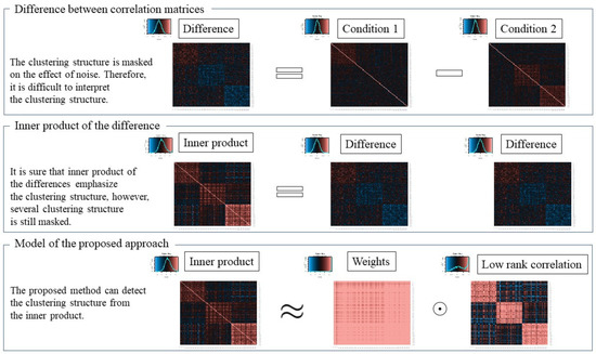
Figure 1.
Image of proposed approach.
In this paper, we propose a new dimensional reduction clustering approach for the inner product of the difference between two correlation matrices. The problem is to estimate both the clustering structure of differences between correlation matrices and the low-rank correlation matrix, which can describe the clustering structure, given two correlation matrices. Our approach has two advantages. First, the clustering results are superior to those from methods that rely only on the difference. Second, the range of the estimated low-rank matrix is bounded within the range to 1, and thus, it is easy to interpret the relations. This approach consists of two steps. First, a low-rank matrix is estimated such that each cluster is discriminated. The novelty of the proposed approach is that the low-rank approximation model is for the inner product of the difference and not only for the difference. From the model, we can estimate the low-rank correlation matrix with features related to the clustering structure. Second, a clustering structure is calculated from the low-rank matrix using an ordinal clustering algorithm such as k-means [14]. A visualization of the proposed approach is shown in lower Figure 1. To address the problem of estimating a correlation matrix from a non-correlation matrix, previous studies have developed a variety of methods [15,16,17,18,19]. In our proposed approach, we need to estimate a low-rank correlation matrix, which indicates the difference between correlations, from the non-correlation matrix. To solve the nearest low-rank correlation matrix problem [20,21,22,23], we adopted and implemented the idea of majorization [20,21] because it eases the estimation of low-rank correlation matrices via the majorization function [24,25].
The remainder of this paper is organized as follows. In the Methods section, the reason for using the inner product of the difference between correlation matrices is discussed, and its advantage over using only the difference is explained. In addition, the proposed model and corresponding objective function are introduced. To estimate the parameters, an algorithm based on the derived majorization function is provided. Afterward, the simulation design of our numerical study and the fMRI data for a mental arithmetic task, for a demonstration of our proposed approach, are described. The results of the simulation and real fMRI data for the mental arithmetic task are discussed. Finally, we offer our concluding remarks regarding the proposed method.
2. Methods
In this section, we explain the proposed method. First, before introducing the optimization problem, we explain our reason for using the inner product of the difference between correlation matrices, instead of using only the difference. The model of the proposed method is then introduced, and the optimization problem of the proposed method is presented. Finally, the simulation design of our numerical study and the fMRI data for a mental arithmetic task, for a demonstration of our proposed approach, are explained.
2.1. Model of Proposed Method
Here, the model of the proposed method is explained. Let , and , be the correlation matrices between variables under condition 1 and condition 2, respectively, where n is the number of subjects and p is the number of variables. From , the difference is calculated as follows:
where . The clustering structure of is assumed to be in the following form:
where is a block matrix such that the absolute values of the elements tend to be higher than those of the elements of , where each element of is 0. That is, is assumed to be changed to Equation (1) through the permutation of these rows and columns.
However, even if has such a clustering structure, the structure is masked because the values are observed with noise, and the corresponding correlations are bounded within the range to 1. Therefore, it is difficult to capture the clustering structure using low-rank approximation based only on . To overcome this problem, the inner product of is focused upon because the clustering structure of the inner product is emphasized, rather than using only . Here, the inner product of is defined as follows:
where the elements of are defined as , and indicates translocation. We focus on the inner product and construct the model based on low-rank approximation from . First, from the property of the inner product, for an arbitrary , there exists such that
where , and is the Euclidean norm. Here, can be considered a correlation, and the matrix representation is
Based on Equations (3) and (4), Equation (2) is expressed as follows:
where , and ⊙ is a Hadamard product.
From Equation (5), we then construct the following model:
where is a coordinate matrix with rank , d is determined by the researchers, and is an error matrix. In addition, the following constraint is added to :
where . From the constraint of Equation (7), becomes the correlation coefficient between i and j with rank d [20,21], and also becomes a correlation matrix with rank d. The reason why becomes a correlation matrix is explained in [15].
To reiterate, the purpose of the proposed method is estimating a low-rank matrix such that the clustering structure is emphasized. To achieve this purpose, is estimated such that the sum of squares for in Equation (6) is minimized.
2.2. Formulation of Proposed Method
In this subsection, we show the proposed dimensional reduction clustering approach based on Equation (6). The proposed method consists of two steps. First, a low-rank correlation matrix, which indicates the difference between two correlation matrices, is estimated. Second, a traditional clustering algorithm such as k-means [14] is applied to to obtain the clustering structure of variables. Although such two-step approaches have already been proposed in [26,27], those methods were proposed for multivariate data, not square matrices.
Afterward, the optimization problem of estimating a low-rank correlation matrix is described. Given and d, the optimization problem is formulated as follows:
where indicates the Frobenius norm. In this study, to estimate such that Equation (8) is minimized with the constraint of Equation (9), the majorize–minimization (MM) algorithm is used.
2.3. Algorithm for Estimating Low-Rank Correlation Matrix Based on MM Algorithm
This subsection provides a detailed description of the MM algorithm for estimating . First, we derive the majorizing function of Equation (8) in the same manner as in [24,25]. The updated formula for is also derived based on the majorizing function. Based on the majorizing function, the problem is then converted into a linear problem. Therefore, the updated formula can be derived via the Lagrange multipliers method with the constraint Equation (9).
However, first, before the derivation the majorizing function is presented, the principle of the MM algorithm is explained. For more details on the MM algorithm, see [24,25]. Let be an objective function with the parameter , and be a real valued function, where is the fixed value of . When satisfies
is said to be a majorizing function. In general, deriving the updated formula for is expected to be easy compared to that for . Therefore, in this proposed approach, the majorizing function of (8) is derived in the same manner as in [24,25].
The objective function Equation (8) can now be defined as follows:
The third term of Equation (10) corresponding to i is expressed as follows:
where . Let be the maximum eigenvalue of . For any with the constraint , the following inequality is satisfied:
where is an identity matrix of size d. That is, is negative semi-definite. Let and be coordinate vectors of subject i corresponding to the current step and the previous step, respectively. Based on Equation (12), the following inequality is satisfied:
If , Equation (13) becomes an equality equation. Equation (13) is substituted into the third term of Equation (10), resulting in
From (14), the updated formula of is derived as follows:
For the algorithm based on Equation (15), see Algorithm 1.
| Algorithm 1 Estimating correlation matrix with rank d |
| Require: Inner product , rank d, initial vectors , and Ensure: coordinate matrix with rank d while do for do end for end while return |
Finally, to detect the clustering structure of the variables, k-means is applied to , with which k clusters on the d dimensions are detected from .
In short, the proposed method can estimate p by d matrix , which is composed of the coordinates of variables on d dimensions, from the inner product matrix with full rank . Therefore, estimating from is considered a dimensional reduction. Furthermore, k-means is applied to such that the rows of are classified into k clusters.
2.4. Simulation Study
In this subsection, the superiority of the proposed method is shown via the results of a numerical simulation. In particular, the recovery of clustering results is evaluated in this simulation.
First, we reveal the simulation design. To evaluate the clustering results, artificial data with a true clustering structure are generated and correlation matrices between variables are calculated from the data. Dimensional reduction clustering approaches are then applied to the difference between the two correlation matrices, and the clustering results are obtained. In this numerical simulation, the true number of clusters is assumed to be known beforehand. Finally, an adjusted Rand index (ARI) [28] between the true clustering structure and the estimated clustering structure is calculated, and the effectiveness of the proposed method is compared with that of existing approaches. Here, ARI is the similarity index between two clustering results. When two clustering results are completely equivalent to each other, ARI becomes 1; otherwise, ARI becomes close to 0.
Afterward, we explain the method for generating the artificial data. Multivariate data representing condition 1 and condition 2 are generated as follows:
where X and Y are random vectors of conditions 1 and 2, respectively; is a vector with length p, for which the elements are all zero; and and are true correlation matrices of condition 1 and condition 2, respectively. Here, in this simulation, p is set to 120. From Equation (16), p dimensional vectors are generated 60 times for each condition, and sample correlation matrices of condition 1 and condition 2 are calculated as and , respectively. The input data are then calculated as .
In this simulation, four factors are utilized; a summary of the simulation is shown in Table 1. As a result, there are patterns in this simulation. For each pattern, the corresponding artificial data are generated 100 times and evaluated using the ARI. The descriptions of the factors are presented as follows.

Table 1.
Summary of simulation design.
- Factor 1:
- Methods
For this factor, we evaluate four methods. The purpose of setting this factor is to evaluate the effect of using an inner product and to estimate a bounded low-rank matrix. Here, the proposed method is referred to as method 1. By contrast, method 2 is designed to have an approach similar to that of the proposed approach, except method 2 is based only on difference and not on the inner product. Through a comparison between the proposed method and method 2, we can evaluate the effect of using the inner product. On the other hand, in method 3, the low-rank matrix is estimated from only the difference and calculated via Cholesky decomposition, where these estimated values are characterized by no constraint. Based on a comparison between the proposed method and method 3, the effect of both the inner product and bounded constraint is evaluated. Meanwhile, in method 4, the low-rank matrix is estimated from the inner product; however, the estimated values are characterized by no constraint. Therefore, based on a comparison between the proposed method and method 4, the effect of the bounded constraints is estimated.
These four methods are then explained from the perspective of calculation. The first method is the proposed approach based on the inner product of . For the second method, an approach based on difference, and not on the inner product model, is adopted. The second method consists of two steps, as does the proposed method. First, is decomposed as using Cholesky decomposition, where . Let ; therefore, there exists such that . From the decomposition, the optimization problem of the second method is formulated as follows:
where . The parameters of Equation (17) can be estimated in the same manner as in the proposed method. Subsequently, k-means is applied to the estimated .
The third method also consists of two steps. Eigenvalue decomposition is applied to , and the low-rank matrix corresponding to is estimated, where are eigenvalues of . Afterward, k-means is applied to the estimated low-rank matrix. The fourth method is similar to the third method, with the only difference being that eigenvalue decomposition is applied to the inner product matrix of and not only to .
These methods, i.e., method 2, method 3, and method 4, are referred to as tandem approaches [29], each of which consists of two steps. First, the existing dimensional reduction method is applied to the data and the low-rank data matrix is estimated. Second, a typical clustering algorithm, such as k-means clustering, is applied to the estimated low-rank data matrix. In a practical situation, these approaches are sometimes used.
Both the third and fourth methods provide us with low-rank matrices and clustering results. However, from these results, it is difficult to interpret the degree of the relation because these estimated values are not bounded. On the other hand, both the first and second methods allow us to interpret the results easily because these estimated values are bounded within the range to 1.
- Factor 2:
- Rank
For the four methods mentioned in the previous subsection, the rank must be determined. In this simulation, ranks are set to , and 4.
- Factor 3:
- Number of clusters
All four methods mentioned in the Factor 1: Methods subsection adopt k-means clustering. In the simulation, we assume that the the number of true clusters is known beforehand. The number of clusters is set to and 4.
- Factor 4:
- Difference between true correlations
At first, the generation of true clustering structures is determined by , and 4. The true clustering structure is dependent on and . When , the equations for and are
where , is a identity matrix, , and if . To reiterate, there are two levels for simulation factor 4. The first level and second level are and , respectively. When , the corresponding difference matrix is more affected by observational error compared to when . With this factor, the degree of effect on the observational error is evaluated.
For ,
where is defined in the same manner as . Finally, for ,
where is defined in the same manner as both and .
With the aforementioned and , a true clustering structure is described. For , and 4, the cluster sizes of each are the same; that is, for , and 4, the cluster sizes are 60, 40, and 30, respectively.
2.5. fMRI Data for Mental Arithmetic Task
Among the cognitive functions, working memory (WM) is important for engaging in everyday tasks such as conversations or reading books. WM is the system for temporally storing and processing necessary information [30,31]. In studies on cognitive function, the neural basis of the WM has been investigated using fMRI. In the current research, the brain regions and functional connectivity networks associated with the WM system are revealed. To validate the effectiveness of the proposed method, we apply the proposed method to fMRI data measured during the WM task.
2.5.1. Participants
Thirty-two healthy adults (20 males and 12 females; mean age, years; 31 right-handed and 1 left-handed) participated in this experiment. This study was approved by the Research Ethics Committee of Doshisha University (approval code: 1331) in Kyoto, Japan. Written informed consent was obtained from each participant.
2.5.2. Experimental Design
The participants were asked to perform a mental arithmetic task in an fMRI scanner. The experimental design is shown in Figure 2. In this experiment, a block design was adopted such that procedures for the rest periods and task periods were conducted alternately. During rest, participants were instructed to watch a fixation point. On the other hand, during the task, they were instructed to press buttons to answer true or false in response to a presented numerical formula. They could proceed to the next formula at their own pace by selecting an answer to the current formula. They performed two types of mental arithmetic tasks, each having a different level of difficulty: (1) low-WM load (Low-WM) tasks, which consisted of addition of one-digit numbers, and (2) high-WM load (High-WM) tasks, which consisted of arithmetic operations on real numbers with three digits. Each of the two task types was performed three times (i.e., each participant performed a total of six tasks in the experiment), and the task order was randomized. The durations of the first rest block, second rest block, and task block were 40 s, 36 s, and 30 s, respectively.
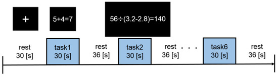
Figure 2.
Experimental design.
2.5.3. Data Acquisition
All MRI scans were performed on a 1.5T Echelon Vega (Hitachi, Ltd.). Functional images were acquired using a gradient-echo echo-planar imaging sequence (TR = 3000 ms, TE = 40 ms, flip angle = , field of view = , matrix size = pixel, thickness = mm, and number of slices = 20). Structural images were acquired using an Rf-spoiled steady state gradient echo sequence (TR = ms, TE = ms, flip angle = , field of view = mm, matrix size = pixel, thickness = mm, and number of slices = 194). The stimuli (fixation point and arithmetic formula) were presented and synchronized with fMRI data acquisition using presentation software (Neurobehavioral System Inc., Albany, CA, USA), and participant responses were acquired using the fORP932 Subject Response Package (Cambridge Research Systems Ltd., London UK).
2.5.4. Data Preprocessing
The first six scans were excluded from the analysis to eliminate the nonequilibrium effects of magnetization. The functional images were preprocessed using SPM12 software (Wellcome Department of Cognitive Neurology, London UK) [2]. These images were realigned to correct for head movements and subsequently slice-timing corrected; anatomical images were then coregistered to the mean of the functional images. The images were also spatially normalized into Montreal Neurological Institute (MNI) space and smoothed using a Gaussian filter (8 mm full width at half maximum).
2.5.5. Functional Connectivity Analysis: Derivation of Correlation Matrices
For the functional connectivity analysis, the functional images preprocessed using SPM12 were further processed using the CONN toolbox [32]. In detail, nuisance regression was performed using an anatomical component-based noise correction method (aCompCor) [33], in which the first five principal components of signals from the white matter and cerebrospinal fluid masks, head-motion parameters, their first-order temporal derivatives, and the main task effect from the task block (modeled as a canonical hemodynamic-response–function-convolved response) and its first order derivatives were regressed to eliminate physiological noise and potential confounding effects of the task responses.
To calculate functional connectivity during the tasks, the preprocessed images were parcellated into 116 regions, including 90 cerebrum regions and 26 cerebellum regions defined via automated anatomical labeling (AAL); the mean Blood-Oxygen-Level-Dependent (BOLD) time course was then calculated for each region. Subsequently, Pearson correlations among BOLD time courses of the 116 regions were calculated and then Fisher-z transformed. As a result, a correlation matrix was constructed for each participant. In this study, we chose 90 cerebrum regions as the ROIs and used the corresponding correlation matrices for the analysis because the WM system is considered associated with the cerebrum regions [34].
3. Results
In this section, we describe the results of the numerical simulations and of applying the proposed fMRI data method.
3.1. Simulation Results
In this subsection, we describe the results of the numerical simulations. Figure 3 shows the results in terms of the number of clusters and ranks for , for which we assume that the true difference is relatively small. Therefore, it is difficult to recover the true clustering structure. The vertical axes represent the results in terms of ARIs. Here, the methods are compared in terms of the medians and interquartile ranges (IQRs) of the ARIs. In Figure 3, the results of the second and third methods, which utilize only the difference and not the inner product, indicate lower performance than that of the proposed method. As the results in Figure 3 show, the model that utilizes the inner product tends to outperform models that focus only on the differences. In particular, for , the results of the proposed method tend to be superior to those of the other methods.
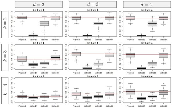
Figure 3.
Simulation result for .
The results for are shown in Figure 4. The tendency of these results is similar to those for , whereas the results corresponding to tend to indicate higher performance than those corresponding to .
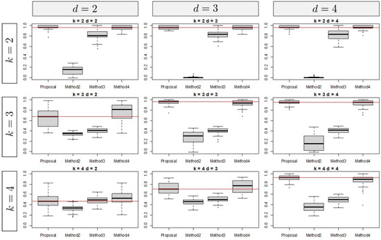
Figure 4.
Simulation result for .
From the overall results, we note two specific observations. First, the number of clusters is relatively large and performance tends to be relatively low, irrespective of the type of method; this tendency has been reported in [35]. Second, all methods depend on the selection of hyperparameters. Based on the simulation results, the tuning parameters should be set to .
3.2. Results of fMRI Data Analysis
In this subsection, we show the results of applying the proposed method to the fMRI data. Concretely, the purpose of this example is to detect clustering structures where the difference between two experimental conditions, i.e., High-WM and Low-WM tasks, is emphasized. In addition, the features of these estimated clusters are interpreted in combination with knowledge on ROIs related to WM, including the task-positive network (TPN), ventral attention network (VAN), salience network (SN), visual network (VN), and default mode network (DMN). The TPN consists of the fronto-parietal network (FPN), dorsal attention network (DAN), and cingulo-opercular network (CON). The FPN and DAN are related to executive function [36] and top-down attention, respectively, whereas the CON is involved in exerting control over the contents of WM [37]. In addition, the VAN is associated with response to stimuli and bottom-up attention, whereas SN activation is said to be observed in situations wherein changes in behavior may be advisable [38,39]. The VN is literally associated with visual information processing, whereas the DMN relates to internally focused tasks such as retrieving autobiographical memory, envisioning the future, and conceiving the perspectives of others [40].
We then explain how to construct the difference between correlation matrices. For each subject, using a matrix of difference between the correlation matrices of High-WM and Low-WM, we calculate one mean matrix of these differences. As described in the previous section, the input difference is a matrix.
In the proposed method, rank and the number of clusters must be selected. For the determination of rank, we set the rank candidates to and 6, and select one among them. Generally, when the rank is larger, the values of the objective function tend to be lower.
The proposed method is then applied to difference matrices of rank , and the rate of change in values of the objective function is calculated as follows:
where is the value of the objective function with rank d. From Figure 5, is selected because, among the candidates, the change in values for the objective function tends not to change even when the rank is larger than 3. For the number of clusters, the silhouettes coefficient [41] is used; the number of clusters that provides the highest silhouettes coefficient is .
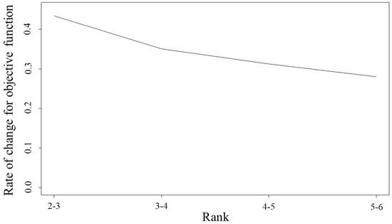
Figure 5.
Change in rate for objective function; vertical and horizontal axes indicate rank and ratio of values for objective function, respectively.
The left side of Figure 6 shows the results of applying the proposed method. Through the estimated low-rank correlation matrix, we confirm that the clustering structure is emphasized and that the relations among ROIs belonging to the same cluster are estimated to be higher. The right-hand side of Figure 6 shows the original difference matrix, in which both rows and columns are permutated by the estimated clusters. The right-hand side of Figure 6 also shows that relations among ROIs belonging to cluster 1 tend to be higher during the difficult task than during the easy task, although those among ROIs belonging to cluster 2 or cluster 3 tend to be lower.
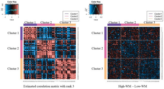
Figure 6.
Estimated correlation matrix for and clustering result; upper-left figure of each heatmap indicates histograms of these coefficients.
The features of the estimated cluster are then interpreted in combination with knowledge on WM. Figure 7 represents the difference matrix (High-WM - Low-WM) permutated based on both estimated clusters and WM. We particularly focused on differences related to the TPN and DMN. For the relations of ROIs belonging to the TPN, those belonging to cluster 1 tend to be higher than those belonging to cluster 2 or cluster 3. Therefore, in cluster 1, correlation among ROIs related to the TPN tended to be active under the condition of High-WM.
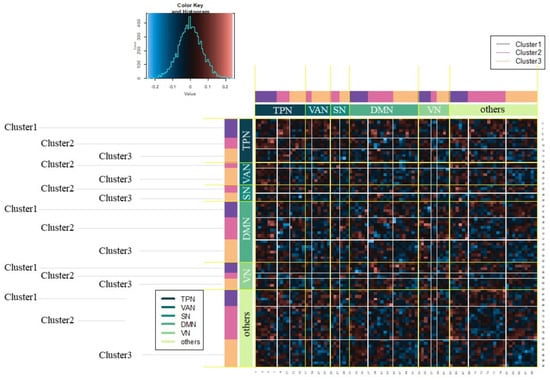
Figure 7.
Difference matrix (High-WM–Low-WM) permutated based on estimated clusters and WM.
These values on Figure 8 are performed to confirm the features of the clusters. In Figure 8, each boxplot represents the differences between ROIs within the WM for each cluster. When correlations within the WM are active in the High-WM condition, the median tends to be greater than 0. On the other hand, when those correlations are active in the Low-WM condition, the median tends to be lower than 0. First, the features of cluster 1 are interpreted. The values corresponding to the TPN in cluster 1 tend to be higher than those in cluster 2 and cluster 3. To reiterate, the TPN includes ROIs within the FPN, DAN, and CON. The connectivities within the FPN tend to be higher in High-WM [42], whereas the DAN is related to top-down attentional control [43]. In addition, there are no ROIs belonging to the VAN or SN as features of cluster 1, where the VAN is related to bottom-up attentional processing. Therefore, cluster 1 is interpreted as comprising ROIs related to top-down attentional control. In cluster 2, there are no ROIs belonging to either the FPN or DAN, and the TPN includes only the CON. The values for the SN in cluster 2 tend to be higher than those in cluster 1 and cluster 3; the SN facilitates access to attention and working memory resources. In addition, the differences corresponding to the DMN tend to scatter around 0 symmetrically. From these features, cluster 2 is interpreted as comprising ROIs related to the SN. In cluster 3, those within the TPN are lower compared to those within the other clusters. In addition, those within the VAN tend to be higher than those in cluster 2, where there are no ROIs within the VAN. Therefore, cluster 3 is interpreted as comprising ROIs related to bottom-up attentional processing.
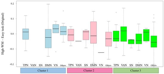
Figure 8.
Boxplot of difference (High-WM–Low-WM) based on estimated clusters and WM.
Although the proposed method was applied to fMRI data during mental arithmetic tasks as an explanatory analysis, these results suggest that our method can detect community structures consisting of well-known functional networks associated with the human working memory system.
4. Conclusions and Remarks
We proposed a new dimensional reduction clustering approach based on differences between correlation matrices. The estimated low-rank correlation represents the difference, and it is easy to interpret the relations because the estimated values are bounded within the range to 1 and because the clustering structure is emphasized. In addition, based on the idea of using the inner product of the difference and not only the difference, we demonstrated that the clustering recovery tends to be accurate. The effectiveness of the proposed method is demonstrated through numerical simulations of the recovery of a true clustering structure. According to these results, the proposed method can detect informative features related to clustering structure and can eliminate noise, and using the low-rank approximation model for the inner product and not only the difference degrades the effect of noise not related to the clustering structure. Certainly, based on the result of numerical simulation, the clustering approach based on eigen decomposition of performs well. However, it is difficult to interpret the estimated low-rank matrix because these values are not bounded.
In addition, we show the results of applying the proposed method to real fMRI data related to WM. Through dimensionality reduction, the clustering structures of the ROIs are emphasized, as shown in the left side of Figure 6, because the variances of these estimated low-rank correlation coefficients tend to be larger. Specifically, our proposed method results in clusters that are interpreted based on knowledge regarding WM.
Finally, we discuss the future direction of this research topic. There are four things to consider. First, although the proposed method certainly provides us with interpretable results from the perspective of WM, the proposed method requires further evaluation through real-data analyses and comparison with other methods. The properties of the clustering results, in particular, should be evaluated through the use of benchmark data. Second, although we show that the proposed method is based on Pearson’s correlation coefficient, other kinds of similarity measures, such as Spearman’s correlation coefficient, should be considered. Third, in the numerical simulations, we evaluate the clustering results using ARI. However, there are several other measures for comparing clustering results [44,45]; these external validation measures are classified into three kinds of measures, i.e., pair counting, information-theory-based approaches, and set-matching measures. In the pair-counting approach, a pair of subjects is regarded as agreeing if the pair belongs to the same cluster in both clustering results or belongs to different clusters in both clustering results; otherwise, these subjects are regarded as disagreeing. In the information-theory-based approach, mutual information measures between two clustering results are used [46,47,48]. On the other hand, in set-matching measures, pairs of clusters are used instead of pairs of subjects; for this approach, several indices have already been proposed [49,50]. Examples of related indices include centroid index [51] and centroid ratio [52]. Therefore, other evaluation indices should be considered for use with our proposed method. Fourth, an ideal number of clusters must be determined. In the real-data example, we used the silhouettes coefficient. However, various methods for determining the number of clusters have also been developed [53,54,55], where the method proposed in [55] is also used for determining the number of dimensions. Further simulations must be performed to better evaluate the effects of these approaches on the results of our proposed method.
Author Contributions
K.T. constructed the proposed statistical method, conducted numerical simulations, applied the method to real fMRI data, and drafted the initial manuscript. S.H. designed and conducted the experiment, proposed the framework of fMRI data analysis, and reviewed the manuscript. Both authors have read and agreed to the published version of the manuscript.
Funding
This work was supported by JSPS KAKENHI grant numbers JP17K12797 and JP19K12145.
Institutional Review Board Statement
Not applicable.
Informed Consent Statement
This study was approved by the Research Ethics Committee of Doshisha University (approval code: 1331), Kyoto, Japan. Informed consent was obtained for all subjects before they enrolled in the experiment.
Data Availability Statement
The artificial data used in the numerical simulations were generated based on probability distribution. For the method of generation, see the subsection Simulation Study. The datasets used in this study are available from the authors upon reasonable request.
Acknowledgments
We appreciate our academic editor and reviewers for their useful comments.
Conflicts of Interest
The authors declare that there are no competing interests.
Abbreviations
The following abbreviations are used in this manuscript:
| AAL | automated anatomical labeling |
| ARI | adjusted Rand index |
| aCompCor | an anatomical component-based noise correction method |
| BOLD | blood-oxygen-level-dependent |
| CON | cingulo-opercular network |
| DAN | dorsal attention network |
| DMN | default mode network |
| EEG | electroencephalography |
| fMRI | functional magnetic resonance imaging |
| fNIRS | functional near-infrared spectroscopy |
| FPN | fronto-parietal network |
| IQRs | interquartile ranges |
| MNI | Montreal Neurological Institute |
| ROIs | regions of interest |
| SN | salience network |
| VN | visual network |
| TPN | task positive network |
| VAN | ventral attention network |
| WM | working memory |
References
- Fillipi, M. FMRI Techniques and Protocols; Springer Protocols, Humana Press: New York, NY, USA, 2009. [Google Scholar]
- Friston, K.; Ashburner, J.; Kiebel, S.; Nichols, T.; Penny, W. Statistical Parametric Mapping: The Analysis of Functional Brain Images; Academic Press: London, UK, 2007. [Google Scholar]
- Ferrari, M.; Quaresunama, V. A brief review on the history of human functional near-infrared spectroscopy (fnirs) development and fields of application. NeuroImage 2012, 63, 921–935. [Google Scholar] [CrossRef]
- Michel, C.M.; Murray, M.M.; Lantz, G.; Gonzalez, S.; Spinelli, L.; Grave de Peralta, R. Eeg source imaging. Clin. Neurophysiol. 2004, 114, 2195–2222. [Google Scholar] [CrossRef] [PubMed]
- Bullmore, E.; Sporns, O. Complex brain networks: Graph theoretical analysis of structural and functional systems. Nat. Rev. Neurosci. 2009, 10, 186–198. [Google Scholar] [CrossRef] [PubMed]
- Sporns, O. Structure and function of complex brain networks. Dialogues Clin. Neurosci. 2013, 15, 247–262. [Google Scholar]
- Varoquaux, G.; Craddock, R.C. Learning and comparing functional connectomes across subjects. NeuroImage 2013, 80, 405–415. [Google Scholar] [CrossRef] [PubMed]
- Lerman-Sinkoff, D.B.; Barch, D.M. Network community structure alterations in adult schizophrenia:identification and localization of alterations. Neuroimage Clin. 2016, 10, 96–106. [Google Scholar] [CrossRef]
- Cole, M.W.; Basset, D.S.; Power, J.D.; Braver, T.S.; Petersen, S.E. Intrinsic and task-evoked network architectures of the human brain. Neuron 2014, 83, 238–251. [Google Scholar] [CrossRef]
- Fränti, P.; Sieranoja, S. K-means properties on six clustering benchmark datasets. Appl. Intell. 2018, 48, 4743–4759. [Google Scholar] [CrossRef]
- Yang, J.; Rahardja, S.; Fränti, P. Mean-shift outlier detection and filtering. Pattern Recognit. 2021, 115, 107874. [Google Scholar] [CrossRef]
- Steinley, D. K-means clustering: A half-century synthesis. Br. J. Math. Stat. Psychol. 2006, 59, 1–34. [Google Scholar] [CrossRef]
- Terada, Y. Clustering for high-dimension, low-sample size data using distance vectors. arXiv 2013, arXiv:1312.3386. [Google Scholar]
- Forgy, E.W. Cluster analysis of multivariate data: Efficiency versus interpretability of classifications. Biometrics 1965, 21, 768–769. [Google Scholar]
- Knol, D.K.; Ten Berge, J.M.F. Least-squares approximation of an improper correlation matrix by a proper one. Psychometrika 1989, 54, 53–61. [Google Scholar] [CrossRef]
- Lurie, P.M.; Goldberg, M.S. An approximate method for sampling correlated random variables from partially-specified distributions. Manag. Sci. 1998, 44, 203–218. [Google Scholar] [CrossRef]
- Malick, J. A dual approach to solve semidefinite least squares problems. SIAM J. Matrix Anal. Appl. 2004, 26, 272–284. [Google Scholar] [CrossRef]
- Qi, H.D.; Sun, D. A quadratically convergent newton method for computing the nearest correlation matrix. SIAM J. Matrix Anal. Appl. 2006, 28, 360–385. [Google Scholar] [CrossRef]
- Borsdorf, R.; Higham, N.J. A preconditioned newton algorithm for the nearest correlation matrix. IMA J. Numer. Anal. 2010, 30, 94–107. [Google Scholar] [CrossRef]
- Pietersz, R.; Groenen, P. Rank reduction of correlation matrices by majorization. Quant. Financ. 2004, 4, 649–662. [Google Scholar] [CrossRef]
- Simon, D.; Abell, J. A majorization algorithm for constrained approximation. Linear Algebra Appl. 2010, 432, 1152–1164. [Google Scholar] [CrossRef][Green Version]
- Grubisic, I.; Pietersz, R. Efficient rank reduction of correlation matrices. Linear Algebra Appl. 2007, 422, 629–653. [Google Scholar] [CrossRef]
- Duan, X.F.; Bai, J.C.; Li, J.F.; Peng, J.J. On the low rank solution of the q-weighted nearest correlation matrix problem. Numer. Linear Algebra Appl. 2016, 23, 340–355. [Google Scholar] [CrossRef]
- Hunter, D.R.; Lange, K. A tutorial on mm algorithm. Am. Stat. 2004, 58, 30–37. [Google Scholar] [CrossRef]
- Borg, I.; Groenen, P. Modern Multidimensional Scaling; Springer: New York, NY, USA, 1997. [Google Scholar]
- Zhang, Z.; Dai, G. Optimal scoring for unsupervised learning. Neural Inf. Process. Syst. 2009, 23, 2241–2249. [Google Scholar]
- Wang, Y.; Fang, Y.; Wang, J. Sparse optimal discriminant clustering. Stat. Comput. 2016, 26, 629–639. [Google Scholar] [CrossRef]
- Hubert, L.; Arabie, P. Comparing partitions. J. Classif. 1985, 2, 193–218. [Google Scholar] [CrossRef]
- Arabie, P.; Hubert, L. Cluster analysis in marketing research. In Advanced Methods of Marketing Research; Bagozzi, R.P., Ed.; Blackwell: Oxford, UK.
- Baddeley, A.D.; Hitch, G. The psychology of learning and motivation. Work. Mem. 1974, 8, 47–89. [Google Scholar]
- Baddeley, A.D. The episodic buffer: A new component of working memory? Trends Cogn. Sci. 2000, 4, 417–423. [Google Scholar] [CrossRef]
- Susan, W.; Nieto-Castanon, A. Conn: A functional connectivity toolbox for correlated and anticorrelated brain networks. Brain Connect. 2012, 2, 125–141. [Google Scholar]
- Behzadi, Y.; Restom, K.; Liau, J.; Liu, T.T. A component based noise correction method (compcor) for bold and perfusion based fmri. Neuroimage 2007, 37, 90–101. [Google Scholar] [CrossRef] [PubMed]
- D’Esposito, M.; Postle, B.R. The cognitive neuroscience of working memory. Annu. Rev. Psychol. 2015, 66, 115–142. [Google Scholar] [CrossRef]
- Milligan, G.W.; Cooper, M.C. A study of standardization of variables in cluster analysis. J. Classif. 1988, 5, 181–204. [Google Scholar] [CrossRef]
- Cole, M.W.; Repovs, G.; Anticevic, A. The frontopaparietal control system: A central role in mental health. Neuroscientist 2014, 20, 652–664. [Google Scholar] [CrossRef]
- Wallis, G.; Stokes, M.; Cousijn, H.; Woolrich, M.; Nobre, A.C. Frontoparietal and cingulo-opercular networks play dissociable roles in control of working memory. J. Cogn. Neurosci. 2015, 27, 2019–2034. [Google Scholar] [CrossRef]
- Dosenbach, N.U.F.; Fair, D.A.; Miezin, F.M.; Cohen, A.L.; Wenger, K.K.; Dosenbach, R.A.T.; Fox, M.D.; Snyder, A.Z.; Vincent, J.L.; Raichle, M.E.; et al. Distinct brain networks for adaptive and stable task control in humans. Proc. Natl. Acad. Sci. USA 2007, 104, 11073–11078. [Google Scholar] [CrossRef] [PubMed]
- Ham, T.; de Boissezon, X.; Joffe, A.; Sharp, D.J. Cognitive control and the salience network: An investigation of error processing and effective connectivity. J. Neurosci. 2013, 33, 7091–7098. [Google Scholar] [CrossRef]
- Buckner, R.L.; Andrews-Hanna, J.R.; Schaacter, D.L. The brain’s default network: Anatomy, function, and relevance to disease. Ann. N. Y. Acad. Sci. 2008, 1124, 1–38. [Google Scholar] [CrossRef] [PubMed]
- Rousseeuw, P.J. Silhouettes: A graphical aid to the interpretation and validation of cluster analysis. J. Comput. Appl. Math. 1987, 20, 53–65. [Google Scholar] [CrossRef]
- Godwin, D.; Ji, A.; Kandala, S.; Mamah, D. Functional connectivity of cognitive brain networks in schizophrenia during a working memory task. Front. Psychiatry 2017, 8, 294. [Google Scholar] [CrossRef]
- Vossel, S.; Geng, J.J.; Fink, G.R. Dorsal and ventral attention systems: Distinct neural circuits but collaborative roles. Neuroscientist 2014, 20, 150–159. [Google Scholar] [CrossRef]
- Van der Hoef, H.; Warrens, M.J. Understanding information theoretic measures for comparing clustering. Behaviormetrika 2019, 46, 353–370. [Google Scholar] [CrossRef]
- Rezaei, M.; Fränti, P. Set matching measures for external cluster validity. IEEE Trans. Knowl. Data Eng. 2016, 28, 2173–2186. [Google Scholar] [CrossRef]
- Meilă, M. Comparing clusterings.an information based distance. J. Multivar. Anal. 2007, 98, 873–895. [Google Scholar] [CrossRef]
- Meilă, M. Criteria for comparing clustering. In Handbook of Cluster Analysis; Hennig, C., Meilă, M., Murtagh, F., Rocci, R., Eds.; Chapman and Hall: New York, NY, USA, 2015; pp. 619–636. [Google Scholar]
- Vinh, N.X.; Epps, J.; Bailey, J. Information theoretic measures for clustering comparison: Variants, properties, normalization and correction for chance. J. Mach. Learn. Res. 2010, 11, 2837–2854. [Google Scholar]
- De Souto, M.C.P.; Hielho, A.L.V.; Faceli, K.; Sakata, T.C.; Bonadia, V.; Costa, I.G. A comparison of external clustering evaluation indices in the context of imbalanced data sets. In Proceedings of the 2012 Brazilian Symposium on Neural Networks, Curitiba, Brazil, 20–25 October 2012; pp. 49–54. [Google Scholar]
- Meilă, M.; Heckerman, D. An experimental comparison of model based clustering methods. Mach. Learn. 2001, 41, 9–29. [Google Scholar] [CrossRef]
- Fränti, P.; Rezaei, M.; Zhao, Q. Centroid index:Cluster level similarity measure. Pattern Recognit. 2014, 47, 3034–3045. [Google Scholar] [CrossRef]
- Zhao, Q.; Fränti, P. Centroid ratio for a pairwise random swap clustering algorithm. IEEE Trans. Knowl. Data Eng. 2014, 26, 1090–1101. [Google Scholar] [CrossRef]
- Tibshirani, R.; Walther, G.; Hastie, T. Estimating the number of clusters in a data set via the gap statistic. J. R. Stat. Soc. Stat. Methodol. Ser. 2001, 63, 411–423. [Google Scholar] [CrossRef]
- Sugar, C.A.; James, G.M. Finding the Number of Clusters in a Dataset: An Information-Theoretic Approach. J. Am. Stat. Assoc. 2003, 98, 750–763. [Google Scholar] [CrossRef]
- Wang, J. Consistent selection of the number of clusters via crossvalidation. Biometrika 2010, 97, 893–904. [Google Scholar] [CrossRef]
Publisher’s Note: MDPI stays neutral with regard to jurisdictional claims in published maps and institutional affiliations. |
© 2021 by the authors. Licensee MDPI, Basel, Switzerland. This article is an open access article distributed under the terms and conditions of the Creative Commons Attribution (CC BY) license (https://creativecommons.org/licenses/by/4.0/).