Modeling In-Match Sports Dynamics Using the Evolving Probability Method

Abstract

The prediction of sport event results has always drawn attention from a vast variety of different groups of people, such as club managers, coaches, betting companies, and the general population. The specific nature of each sport has an important role in the adaption of various predictive techniques founded on different mathematical and statistical models. In this paper, a common approach of modeling sports with a strongly defined structure and a rigid scoring system that relies on an assumption of independent and identical point distributions is challenged. It is demonstrated that such models can be improved by introducing dynamics into the match models in the form of sport momentums. Formal mathematical models for implementing these momentums based on conditional probability and empirical Bayes estimation are proposed, which are ultimately combined through a unifying hybrid approach based on the Monte Carlo simulation. Finally, the method is applied to real-life volleyball data demonstrating noticeable improvements over the previous approaches when it comes to predicting match outcomes. The method can be implemented into an expert system to obtain insight into the performance of players at different stages of the match or to study field scenarios that may arise under different circumstances.

1. Introduction

Although predicting the outcome of sporting events has always been of great interest to people, it has gained even more popularity with the advancement of the Internet and the introduction of live betting. Historically, domain experts have had the main role in producing such predictions. Based on accumulated experience, domain familiarity, and currently available data, domain experts would manually come up with predictions. However, relying on human expertise and manually generated predictions is neither a scalable nor a cost-effective solution. Additionally, domain experts are usually not able to produce predictions in a time-critical fashion. Recently, with the increase in the processor power and storage capacities of modern information systems coupled with the developments in the field of predictive data analytics, computers are taking over the main role in predicting the outcomes of sports events—not only regarding the final results, but also concerning various events occurring during the match.

Predictive analytics has to date been successfully applied to various sports, from football [1,2] and basketball [3,4], to hockey [5], cricket [6], and rugby [7]. The nature of each sport greatly influences the adaption of advanced techniques to be used for prediction. Sports with a strongly defined structure and a rigid scoring system are especially suitable for this purpose since it is relatively easy to model them in the form of discrete stochastic processes, such as a Markovian process [8]. Due to this fact, in the rest of this paper, such sports will be referred to as discrete or Markovian sports. Typical examples of such sports are tennis and volleyball. Papers dealing with this approach usually choose tennis for modeling [9,10]. In this paper, the focus will be put on volleyball since it has been relatively scarcely presented in scientific papers to date. Despite this fact, shown principles are generalizable and can be applied to other discrete sports which use a similar, tightly defined scoring scheme.

Most published approaches focus on building models (pre-match and in-play) which base their estimates of match outcomes on historical data and the known average service percentages of both teams. These values are precomputed and subsequently fed to mathematical equations based on a Markov chain to produce the probability of a given team winning the match or to estimate the duration of the match in terms of the total number of points that will be played in the match. These models are created with the common assumption that points in discrete sports are identically and independently distributed (commonly called the iid distribution). This means that the average service percentages of both teams, once calculated from historical data, never change throughout the match whose outcome is to be predicted. The notion of independence stems from the presumption that the probability of winning a point on serve is not influenced in any way by the outcome of previous points. The assumption that each point is equal, regardless of whether it is a point of little importance at the beginning of the match or a crucial point in the final set, is the identical part of the iid annotation. Schutz [11] was the first to describe a tennis match through a Markov chain with constant probabilities of transition between states. Pollard [12] presented an analytical approach that was used to calculate game, set, and match win probabilities. He also obtained solutions for the mean and variance of the number of points played in a game, set, and match, respectively. After that, many more papers were published that also proposed solutions to predict the outcome of tennis matches, either before the match started, pre-match models [9,13,14], or during the match whose outcome is to be predicted, or in-match models [15,16,17,18]. Although tennis has been the main focus in Markovian sports modeling, there are also papers that focus on volleyball analysis. The milestone of volleyball analysis was published in 2004 [19], where the authors derived expressions for set winning probability in terms of the Legendre polynomials. They also showed the importance of information about who is serving first in a deciding set in volleyball. Barnett et al. [20] had a first attempt to estimate the set winning probabilities and the duration of a volleyball set (in terms of the number of points played in a set) using the Markovian chain model. They offered recurrence formulas to estimate those values. Ferrante and Fonseca [21] refactored the previous paper from the combinatorial point of view, while making a distinction between the two scoring systems. A common assumption which all these papers are based on is the identical and independent distribution of points.

The assumption of the independent and identical distribution of points greatly facilitates the modeling of volleyball and tennis matches, but conflicts with a phenomenon very popular in psychology—psychological momentum [22]. Since the end of the twentieth century, the existence of psychological momentum has been a topic of research in the sports domain, where the synonymous term “hot-hand” is used more often. Briefly, “hot-hand” or psychological momentum is a belief that a player has a higher chance of scoring a point after a few successful points. The research has been conducted on a variety of sports, mainly in basketball [23,24,25,26], baseball, [27] and tennis [28,29,30,31,32,33,34,35]. Quite extensive research on the existence of psychological momentum has also been conducted in volleyball [36,37,38]. It is almost impossible to watch a match without the sports commentator mentioning the term “hot hand” or “hot team” at least once during a match. Observing the number of time-outs that the coach calls during matches after several good consecutive moves of the opposing team, it is evident that the coaches also believe in the existence of psychological momentum. Although it is a very intuitive concept, believed by a larger group of non-professionals, in scientific research the belief in the existence of psychological momentum is still divided (Bar-Eli et al. [39] have written an excellent review). This paper assumes that the momentum exists in volleyball and proposes a predictive method that incorporates a short-term boost in the likelihood of winning a point on one’s own serve after a motivating event happens. This will be referred to as short-term momentum. Ultimately, an analysis is performed of how this assumption affects the outcome prediction of volleyball matches and the results are compared with models based on the iid assumption.

Barnett et al. [40] proved that predicting the outcome of a tennis match is more effective by combining historical and current match data. Barnett et al. [41] and Kovalchik and Reid [42] proposed in-match prediction methods used to update the pre-match tennis statistics with in-match information as the match progresses. This paper uses volleyball matches to prove the importance of combining the historical statistics of the team and the statistics computed from the currently simulated match through the long-term momentum formulation.

When building any predictive model, the quality of results will mostly depend on the model input. In the analysis of volleyball and tennis matches, the likelihood of winning a point on its own serve proved to be one of the most important features. Many papers have focused on how to accurately determine this parameter. Barnett and Clarke [43] proposed methods for combining player statistics using averaged player serve percentages with an average serve percentage by tournament which proved to be an important scaling parameter. Newton and Aslam [44] also proposed a similar method for combining player statistics using the assumption that a service win percentage between matches has a Gaussian distribution which results in an option to expand input parameters with standard deviations of four service percentages. They used the Monte Carlo simulation to create/simulate data for players with a small number of matches. Knottenbelt et al. [10] introduced a common opponent method which should further enhance input parameters if sufficient enough data are available. In the case of a small dataset, it is possible to recursively average statistics over common opponents or go even deeper. Ingram [45] presented a Bayesian hierarchical model used to predict the probability of winning a point on a serve given surface, tournament, and match date. The approach presented in this paper also uses the probability of winning a point on its own serve as one of the input parameters. Due to the size and heterogeneity of the used dataset, the proposed method is based on profiling groups of matches rather than individual teams in order to obtain the input parameters. Details will be given in Section 2.7.1.

Carrari et al. [46] show that this area of research is still up to date and that, in various ways, scientists try to prove that modeling discrete matches using the iid assumption does not give precise results. In that paper, the tennis match is modeled in the way that the probability of a player winning their own service is divided into two categories: starting points and decisive points. Percy [8] addresses the iid problem and introduces within-game and between-game dynamic learning. In addition, proving the existence of psychological momentum remains a current topic of scientific research [47,48,49].

Sports analytics can also be used to improve players’ performances or to analyze players’ health and injury probabilities. Kautz et al. [50] presented a convolutional neural network (CNN)-based approach for activity recognition in beach volleyball which can be used to identify and understand risk factors and prevent injuries. Khaustov and Mozgovoy [51] proposed an approach for identifying several types of events in soccer. Baclig et al. [52] used video tracking techniques to quantify squash kinematics and tactics. Bendtsen [53] proved that baseball players go through different regimes throughout their career and that each regime can be associated with a certain level of performance. Andrienko et al. [54] proposed a computational approach, which based on the player’s position, calculates the pressure value imposed on the ball or the player. The method presented in this paper can be very easily incorporated into expert systems to gain insight into possible match score sequences that may arise under different circumstances. Experts in the sports domain can use the simulations to identify, understand and optimize player performance.

In the following sections, an approach that substitutes the iid-distribution with non-iid distribution will be introduced, denoting that the points are no longer identically distributed since they need to account for the effect of short- and long-term momentums. The proposed methodology for implementing short- and long-term momentums separately, and ultimately combined will be explained. Short- and long-term momentum will be combined through a single unifying hybrid formula that will be encapsulated within the proposed evolving probability method. To validate this approach, real historical data pertaining to volleyball matches will be used and a comparison of the real-world results with those gained by Monte Carlo simulations of volleyball matches using both the iid-based and non-iid-based approaches will be performed.

2. Materials and Methods

Despite the mathematical attractiveness of the iid approach, the findings in this paper challenge its ability to describe volleyball matches accurately and in a sufficiently flexible fashion. It can be stated that a sports prediction method should combine pre-match information and simulated in-match information as the simulation progresses. The current models can be improved by considering the changes in probabilities of winning a point on serve for each team throughout the match by gradually adjusting the pre-match expectations based on simulation sequences using the empirical Bayes updating rule. This adjustment should have an increasingly larger influence the larger the disparity between historical data and simulated current events is evidenced. This gradual adjustment effect will be referred to as long-term momentum. Additionally, the phenomenon from the field of psychology known as the effect of psychological momentum [22] should also be integrated into match models, through a proposed notion called short-term momentum. This short-term momentum describes situations in which the outcome of a certain event may have a short-term impact on the player’s performance immediately following said event. This basically means that a slight yet noticeable short-term boost in players’ performance may become evident after winning one or more points, and an accurate predictive model should account for it in a certain way. In essence, the appearance of an event should cause a short-term update of the serve point winning probabilities during the match whose outcome is being predicted. A more detailed explanation is given below.

2.1. Volleyball Rules

Before explaining the methodology, a brief overview of the basic volleyball rules and terminology will be provided.

Each team has 6 players on the court who try to score points by grounding a ball on the other team’s court under organized rules. A player on one of the teams begins a “rally” by serving the ball. The team that wins the rally is awarded a point and serves the ball to start the next rally. A team can win a rally if a team makes a kill, grounding the ball on the opponent’s court; or a team commits a fault and loses the rally. The most common faults are hitting the volleyball out of bounds, two consecutive contacts with the ball made by the same player (double hit), four consecutive contacts with the ball made by the same team, touching the net during play (net foul), and stepping over the boundary line when serving (foot fault).

The volleyball game consists of sets. Matches are best-of-three sets or best-of-five sets (scoring differs between leagues, tournaments, and levels). Every set is played to 25 points and must be two points clear (the exception is the fifth set, if necessary, in the best-of-five sets which is played to 15 points). This means that if the score reaches 24-24 (15-15 in the fifth set), the set is played until one team achieves a two-point lead. To win the set, one must score more points than the opponent team, and to win a match, a team must win more sets than the opponent team.

2.2. A Brief Introduction to the iid Model

The iid model applied on discrete sports matches relies on a very simple assumption—the probabilities of winning or losing a point (or a serve) are constant throughout the match. In other words, each point is completely independent of the current state of the match or the events that caused the acquisition of the point which preceded it.

The iid assumption has the benefit of making the process of model building relatively simple and straightforward, assuming the analyst has access to historical data about opposing teams in a match being modeled. Historical averages of winning serves are calculated and then used as probabilities of moving between states in a Markov process model.

An illustration of the iid-based model is shown in Figure 1 (throughout the paper, serve winning probabilities for home and away teams will be denoted as p and q, respectively, which is consistent with the notation already used in [19]). If the data do not allow to discern which team was the “home” team (or the usual definition of “home” team is not applicable to the sport or match in question), the team whose historical statistics showcase advantage over the other team will be proclaimed as the “home” team. In cases of evenly matched teams, the “home” team notion will be applied arbitrarily. This, while not being ideal, is important because it allows keeping the notation consistent throughout all the matches (in all available data), which depicts a Markov model for the first three points of a volleyball match (the way of modeling subsequent points can be easily extrapolated). Each state depicts a score and the star denotes which team was on serve.

As stated, simplicity is the main benefit of this model, and the results may show that it is efficient and serviceable in many scenarios. However, there is a certain amount of proof that assumptions which iid uses may be challenged when examining real-life matches or through analyzing fine-grained historical statistics of sports matches. Klaassen and Magnus [34] have demonstrated that the probability of winning a point is larger when the players have won the previous point (the aforementioned short-term momentum). Additionally, perhaps there is an interest in predicting events in real-time, during the match itself, or someone wants to create more fine-grained predictions beyond just the fact of who will win (for example, a popular betting goal is trying to predict the total number of points that will be played in the match). In most cases, in addition to predicting the final result, experts in the sports domain want to analyze potential score sequences of the match. In this scenario, a strong case can be made for short-term boosting of probabilities of winning a point after a point was just won (from now on referred to as short-term momentum) or long-term adjustment of historical probabilities based on currently available data (long-term momentum). In the following paragraphs, an explanation of the additions that tackle these challenges in an efficient, streamlined fashion will be provided.

2.3. Short-Term Momentum

The short-term momentum represents a brief above-average performance of a team after a certain motivating event happens in the match. Scientists have explained this through the psychological momentum phenomenon, better known as “hot hand” in the sports domain. In tennis, scientists usually consider this motivating event to be the win of a game or a set [29,55,56]. Raab et al. [38] considered a more fine-grained approach in volleyball and examined the hot hand effects at the point level. They used two different measures for proving the existence of a hot hand in volleyball matches: conditional probability and runs test. The same approach has previously been seen in basketball [23].

The research described in this paper also uses conditional probability and available historical data to explore the team’s reaction after winning one or more points in a row on their serve. Therefore, the short-term momentum of the first order is calculated as the conditional probability of winning the second point in a row after the team has won the first point. Similarly, the short-term momentum of the second order is calculated as the conditional probability of winning the third point in a row after the team has previously won two points in a row, etc. However, unlike Raab et al. [38], the idea of this paper is not to test the existence of the hot hand, but to build a probabilistic model that implements the short-term boost phenomenon as an increase in point-winning likelihood on one’s serve, and demonstrate that such a model performs better compared to one that does not recognize this phenomenon. Before modeling the short-term momentum itself, an extensive exploratory analysis on available discrete sports data was performed. Real-life volleyball match data were used to test the following two assumptions, which are required to rationalize the need for the short-term momentum:

• If a team wins a point, a short-term “boost” effect appears which can be represented as the probability of winning the next point becoming slightly larger;
• The boost effect is cumulative, meaning that winning more points in a row will result in an even larger probability of winning the next point

Before demonstrating the results, new terms will be defined.

Motivating events that are primarily considered are one or more consecutive points won on a team’s own serve which lead to winning the next point in sequence. Momentum order (i) indicates the number of such consecutive points. For example, i = 2 means that the serving team has won three points in a row, i.e., the motivating event of winning two consecutive points has occurred, and that the event led to winning the third point. The number of momentum occurrences ($N_i$) represents how many times the momentum of i-th order appeared (per team) during a match. Momentum value ($m_i$) is a number that indicates how much the probability of winning the next point on the team’s own serve is increased, compared to the previously established serve probability, if the serving team has previously won i points in a row. When the team who is on serve wins i points on one’s own serve, the probability of winning the next point on serve will be calculated using Equations (1) and (2). Equations (1) and (2) are based on previously calculated momentum values, $m_i$ (the equations are explained in more detail below).

Figure 2 shows the dependence of the momentum value ($m_i$) on the momentum order (i) of an average volleyball team. For example, the $m_2$ value is a number that represents how much (in percentage) the probability of winning the third point will increase, in relation to the average probability of winning points on the team’s own serve, if the team previously won two points in a row. Figure 2 confirms the hypothesis that a short-term boost effect exists and that it is cumulative. Winning more points in a row will result in a larger probability of winning the next point.

Figure 3 shows the number of momentum occurrences ($N_i$) in an average match for an average team depending on the momentum order (i). For example, the $N_2$ value represents the number that tells how many times the team has won three points in a row. By analyzing Figure 3, it is evident that momentums of the fourth order and beyond appear extremely rarely during the matches in the dataset used in this research. This means that the low number of observations pertaining to these momentums does not provide statistically relevant results. For this reason, the evolving probability method proposed in this paper implements the short-term momentum only up to the third order, even though the method can be very easily extrapolated to work with momentums of higher orders if desired.

Note: The values themselves on Figure 2 and Figure 3 are not as significant in demonstrating the general trend of the relationship. These values are discussed in more detail in Section 2.7.1.

Since the real-life data (see Figure 2) provide enough evidence to rationalize the introduction of the short-term momentum, an approach to mathematically model it using available historical data is devised.

If there are enough historical data available, the historical probability of winning a point on serve for a particular team can be calculated. This will be referred as $p_{hist}$ and $q_{hist}$. If the existence of the short-term momentum is assumed, one can also calculate the short-term momentum values as explained before (conditional probabilities). These values will be called $m_1$, $m_2$ and $m_3$.

Let us start with two variables, $p_{hist}$ and $q_{hist}$. In this paper, these values are calculated as probabilities of winning a point after a break. This was chosen simply because, by definition, the points after the break are the first points in a row and as such do not include the short-term momentum based on the way it is defined in this paper.

Then, when the team who is on serve wins a point, the probability of winning the next point on serve is adjusted, exchanging $p_{hist}$ with the new probability $p_{stm}$, or $q_{hist}$ with the new probability $q_{stm}$, depending on which team was on serve (the letters stm denote “short-term momentum”)—see Equations (1) and (2):

$$p_{stm}=p_{hist}\ast (1+m_i^p)$$

(1)

$$q_{stm}=q_{hist}\ast (1+m_i^q)$$

(2)

The index i represents the momentum order and can acquire values 1, 2, or 3 depending on how many points in a row the team in question has won, and letters p and q refer to the home and away team, respectively, in accordance with the previously established notation (note: p and q in the expression do not signify the exponentiation, but the team the momentum value is related to). As stated previously, these momentum parameters are calculated from historical data before the match (if enough data are available). To keep the calculations simple, momentum values are kept constant during the match and do not consider the potential importance of the specific point being won considering its role in the match, and how it may affect the momentum value itself.

With enough historical data, implementing this approach should be rather straightforward. However, the specifics of each sport should be taken into consideration when handling the short-term momentums themselves. For example, in the case of volleyball, it is enough to analyze the short-term momentum after a team’s serve. This stems from the fact that volleyball rules dictate rotating serves after each lost serve. Additionally, in this sport, the team line-up changes very frequently, so a short-term momentum happens when either a good server is on the turn to serve (so a point is immediately scored) or a well-trained lineup is doing a good job following that serve, turning it into a point. Certain other sports (such as tennis) may have a completely different match dynamic, so a chosen lag window might pertain to all points played in a current game or set.

2.4. Long-Term Momentum

Short-term momentum will not adequately represent situations when events on the field strongly deviate from historical statistics. This can happen for various reasons, which may or may not be reflected in data about the match—for example, a strong team could be missing key players due to injuries, resulting in a poorer performance compared to what historical statistics show, and the model which uses only historical data may continue to favor them more strongly than it should. To account for situations like these, it is important to combine historical match data and available data about the match whose outcome is being predicted. Several papers have already proposed approaches for updating the pre-match data with new information in tennis [40,41,42].

In this paper, the notion of “long-term momentum” is proposed. This momentum dynamically adjusts the historical serve-winning probability using the updating rule which leverages empirical Bayes estimator and currently simulated match results. The idea is to simulate all potential score sequences of the match whose outcome is being predicted. This effectively means that the probability of winning a point is slightly adjusted after each point in the match simulation, so if the team is on a losing streak, the probability of winning the next point may gradually become significantly lower than the average point-winning probability gained from historical statistics, better reflecting what is actually going on in a match simulation.

To integrate the long-term momentum in the proposed model, a new tuning parameter $\lambda$ is introduced, which will represent the size of the long-term momentum effect on the point-winning probability. The long-term momentum has to behave in such a way that historical probability always has the largest influence at the beginning of the match, which then diminishes as the match simulation progresses—especially if the currently simulated match events strongly deviate from what historical statistics state. To model this without introducing a lot of unnecessary complexity, a simple linear interpolation is used, with the interpolation parameter being the current number of points in the match simulation ($totalPt{s}_{current}$) divided by the parameter $\lambda$. The new probabilities are called $p_{ltm}$ and $q_{ltm}$ (ltm denoting “long-term momentum”)—see Equations (3) and (4). Quantities $p_{current}$ and $q_{current}$ are also introduced, which are the probabilities of winning one’s serve using only information from the currently simulated match—in effect, a ratio between the points won on the team’s own serve and the total number of serves, for each team, respectively:

$$p_{ltm}=\frac{totalPt{s}_{current}}{\lambda }\ast p_{current}+(1-\frac{totalPt{s}_{current}}{\lambda })\ast p_{hist}$$

(3)

$$q_{ltm}=\frac{totalPt{s}_{current}}{\lambda }\ast q_{current}+(1-\frac{totalPt{s}_{current}}{\lambda })\ast q_{hist}$$

(4)

The choice of $\lambda$ parameter allows the ability to choose how strongly the long-term momentum will influence the point-winning probabilities. Choosing larger values of $\lambda$ makes historical statistics have a larger impact, while lower values put more emphasis on what is currently simulated. The logical question that arises is how to choose the value of this parameter, or, in other words, how to estimate which values of $\lambda$ would work best based on the a priori information about the match.

Due to the nature of volleyball, the difference in team strengths directly influences the number of points. A simple yet effective approach is to choose the value of parameter $\lambda$ concerning the rough estimate of the expected number of total points. There is logical reasoning behind this if the nature and rules of volleyball are considered. If two teams of similar strength and ability are playing, a much longer match is expected, compared to a match that pits severely imbalanced teams with an obvious favorite against each other. Using this logic, in longer matches, the long-term momentum becomes more and more pronounced which should be reflected in increasingly larger values of $\lambda$. Historical statistics for estimating this number of points can be used, either by using data about the same matchup (if it has happened enough times), or by first grouping the teams based on team strength and calculating an average number of points between teams of defined strengths (an approach which will be demonstrated in Section 2.7.1).

In short, if one does not want to use an arbitrary value for $\lambda$ parameter, and they have enough historical data available, they can model $\lambda$ as a linear function of the estimated total number of points that will be played in the match. The new equation with a modified $\lambda$ is shown bellow in Equations (5) and (6), where the added parameters (k, l, and $totalPt{s}_{exp}$) are calculated from historical data, and k and l are treated as universal parameters for all matches (a more refined approach with conditional k and l, which would be dependent on individual match properties, is being reserved for future research):

$$p_{ltm}=\frac{totalPt{s}_{current}\ast p_{current}}{k\ast totalPt{s}_{exp}+l}+(1-\frac{totalPt{s}_{current}}{k\ast totalPt{s}_{exp}+l})\ast p_{hist}$$

(5)

$$q_{ltm}=\frac{totalPt{s}_{current}\ast q_{current}}{k\ast totalPt{s}_{exp}+l}+(1-\frac{totalPt{s}_{current}}{k\ast totalPt{s}_{exp}+l})\ast q_{hist}$$

(6)

Now, having presented the concepts of short-term and long-term momentums, an approach that combines these two concepts will be introduced.

2.5. Combining Short- and Long-Term Momentums

The combined formula intends to update the serve probabilities of both teams in a volleyball match by combining the historical statistics and the statistics of the currently simulated match (i.e., long-term momentum), while at the same time updating the newly calculated probabilities depending on the occurrence of events which also cause a short-term change in the service statistics (i.e., short-term momentum).

To implement the combined function for modeling the non-iid distribution, Formulas (1) and (5) are combined, treating $p_{hist}$ from Formula (1) as $p_{ltm}$ in Formula (5). The same formula can be written for the away team, treating $q_{hist}$ from Formula (2) as $q_{ltm}$ in Formula (6):

$$p=\left[\frac{totalPt{s}_{current}}{k\ast totalPt{s}_{exp}+l}\ast p_{current}+\left(1-\frac{totalPt{s}_{current}}{k\ast totalPt{s}_{exp}+l}\right)\ast p_{hist}\right]\ast \left(1+m_i^p\right)$$

(7)

$$q=\left[\frac{totalPt{s}_{current}}{k\ast totalPt{s}_{exp}+l}\ast q_{current}+\left(1-\frac{totalPt{s}_{current}}{k\ast totalPt{s}_{exp}+l}\right)\ast q_{hist}\right]\ast \left(1+m_i^q\right)$$

(8)

where the symbols denote the following:

$p_{hist}$($q_{hist}$)

—the probability of winning a point on own serve for the home (guest) team calculated from historical data;

$p_{current}$($q_{current}$)

—the probability of winning a point on own serve in the current match for the home (guest) team;

$m_i^p$($m_i^p$)

—the momentum parameter that determines how much the serve probability would further increase depending on the event of winning one, two or three points in row for the home (guest) team (if $i=0$, $m_i^p=0$ ($m_i^q=0$), if $i>3$, $m_i^p=m_3^p$, ($m_i^q=m_3^q$));

$totalPt{s}_{exp}$

—the expected total number of points that will be played in the match between the teams of known strength ratio calculated from historical data;

$totalPt{s}_{current}$

—the total number of points played in the current match;

k,l

—parameters of the linear function.

Figure 4 shows a match tree that incorporates the proposed combined Formulas (7) and (8). The figure shows the changes of serve probabilities throughout the match for both teams. In order to demonstrate the example, a match with the following characteristics is selected: $p_{hist}=35.03\%$, $q_{hist}=34.47\%$, $m_1^p=2.28\%$, $m_2^p=21.77\%$, $m_3^p=31.75\%$, $m_1^q=5.51\%$, $m_2^q=13.97\%$, $m_3^q=34.58\%$ and $totalPt{s}_{exp}=179$. Values $k=1$ and $l=0$ are selected as the parameters of the linear function. In the approach proposed in this paper, after each rally, the non-constant input parameters of the proposed functions (7) and (8) are updated. Those parameters are the following: $totalPt{s}_{current}$, $p_{current}$ and $q_{current}$. After updating the values, Equations (7) and (8) are used to calculate the probabilities of winning a point on a team’s own serve. Each state has exactly two exclusionary transition probabilities, so it is possible to describe a volleyball match as a binary tree where each leaf represents a non-unique match result and all nodes with the same number of total points are at the same tree depth.

After the presentation and description of the formula that combines short- and long-term concepts, the next section will describe how to leverage this formula to produce match-winning predictions. For this purpose, a Monte Carlo simulation of a volleyball match is performed.

2.6. The Evolving Probability Method

As stated before, this paper aimed to prove that, by introducing dynamics into the model through the short-term and long-term momentums, it is possible to more accurately simulate the real flow of a match. This can then be used to better estimate the outcome of a match, either by choosing the winner of a match, estimating the handicap (the difference in total points won by the favorite team), or the total number of points that will be played in a match. These predictions should be more refined compared to those obtained with models based on the iid assumption. Since making more fine-grained predictions is one of the goals of sports data mining, the emphasis will be on predicting the handicap and the total number of points expected to be played in a match.

To predict these values, and based on methodology introduced in the previous sections, an approach that traverses through a match tree while updating the transition probabilities after each transition using the Equations (7) and (8) is proposed. This Monte Carlo simulation method that incorporates the proposed combined formulation will be called the evolving probability method.

The exact method is as follows: one single simulation generates one match tree that represents one possible flow of the match. From that tree, it is easy to calculate the handicap and the total number of points played in such a simulated match. The simulation of the same match can then be repeated numerous times, and ultimately, the results of all simulations of the match are combined to estimate the handicap and the total number of points that will be played in the match. This method will be formalized through a procedure called The evolving probability method (see procedure The evolving probability method in the Appendix A).

To simulate a match using the proposed evolving probability method, it is necessary to describe the match with certain numerical parameters which represent the performance profiles of the teams playing the match. These profiles are built from historical data. More about the profile construction is given in Section 2.7.1.

2.7. Validation Dataset

In order to evaluate and validate the proposed evolving probability method on real-life data, a dataset pertaining to a number of volleyball matches was collected from the MarathonBet betting house (https://www.marathonbet.com, accessed on 1 May 2021). This dataset contains data about matches played between April 2016 and October 2017. More importantly, this dataset contains in-play changes in the score and the corresponding betting odds made by the betting house itself. For each match score, expected values and odds are stored for three different bet types—match win, expected total points and expected handicap. Odds on winning the match before the match started (so-called pre-match odds) are also available in this dataset. The dataset is publicly available [57]. Used attributes of the dataset are described in

Table 1. Attribute description.

Attribute Name	Description
SportEventID	The unique identifier of every sport event
Score	The score in sets and points marked with * on the side of the team that serves (e.g., $1-2\ast 23-20$)
Pre-matchCoef1/ Pre-matchCoef2	Odds on winning the match for both teams placed before the match started
CoefMatchWin1/ CoefMatchWin2	Odds on winning the match for both teams from the current result in the match
Handicap	Pre-match prediction of approximately expected difference in total points won by favored team in the match
HandicapUnder	Odds that handicap will be lower than Handicap number
HandicapOver	Odds that handicap will be greater than Handicap number
TotalPoints	Pre-match prediction of approximately expected total point number in the match
TotalPointsUnder	Odds that sum of total points will be lower than TotalPoints number
TotalPointsOver	Odds that sum of total points will be greater than TotalPoints number

.

Even though this dataset contained a wealth of information about the domain of interest, after the data cleaning process, data about 4704 individual matches were left.

The dataset lacked information about every change of the score in the match. Since these changes were important for the model, data about matches which did not have this information were eliminated. For the analysis, only matches with the known final result, and matches containing at least 75 in-play changes of the result were selected.

The second issue was the lack of pre-match odds for every match. To avoid further reduction in the dataset, a workaround for indirectly calculating this missing information was employed. The pre-match betting odds from odds set on the following scores: (setHome:setGuest pointHome:pointGuest): 0:0 0:0, 0:0 1:1, 0:0 2:2 were infused. This method was supported by the assumption that the pre-match odds did not change when the match had just started since neither team previously showed better performance during the match.

The initial dataset contained four broad categories of matches (i.e., four different underlying point distributions). More specifically, the dataset contained records about the regular and young section as well as records about male and female competitions. They were firm reasons to believe that the specifics of each subcategory were distinct enough that modeling them together would not be a feasible approach (for example, it has already been shown in sports research that there were noticeable differences between the ways men and women perform their serves and receives [58]). Similarly, differences between young and regular sections were also expected. To ensure a sample of data with matches that have similar underlying point distribution, and to ensure that the simulations can approximate real-world events, a subset of data belonging to one of these groups was used. Taking into account the total number of observations per group, a subset of men volleyball matches excluding the matches from the young section was finally chosen. The chosen men regular section represents 55% of the initial dataset, which ultimately resulted in a set with 4704 individual matches.

2.7.1. Group Profiling

It is a well-known fact that the final results can only be as good as the quality of input data allows it, regardless of the predictive model used. In the analysis of volleyball matches, the service proved to be one of the most important features. When models are implemented in betting systems, analyses at the team, player, or tournament level have to be periodically re-run to ensure model precision. Simple ranking systems and averaged statistics are often not enough, and their results tend to be misinterpreted even by some of the leading betting houses. Home–away statistics and reactions fluctuate from player to player, team to team, and coach to coach.

In an ideal scenario, enough historical data to construct a profile of team performance over a longer time for each team would be available. Then, these data can be used to calculate the likelihood of winning the point on own serve, the parameters of the short-term momentum for each team, as well as the rough estimate of the expected number of total points used to calculate the long-term momentum. These parameters can then be used as input parameters of the proposed evolving probability method to estimate the handicap and the total number of points that will be played between two teams.

In the case of this paper, however, the heterogeneity of the available dataset did not allow leveraging this simple approach. The collected dataset did not contain enough information on the historical matches of most teams. Since acquiring a significantly larger dataset was not feasible, it was decided to devise with a method that would most efficiently compensate for the relatively low number of observations (when taking into account the needs for team profiling). The approach proposed in this paper was to exchange the notion of individual team profiling with building group profiles, but in a way that does not group teams—individual matches in which opposing teams have a similar strength ratio are grouped. For example, one of the groups contains matches with a strong favorite, while the other contains matches in which teams of similar strengths are opposed. It is important to notice that in this way it is possible to leverage the dataset much more efficiently and that now, individual teams are naturally represented in more than one group since they have different strength ratios when pitted against different teams. In this way of profiling, the strength of the opposing team is taken into account, and it is not necessary to take additional care of it. This means that the same team will have a different profile depending on the opposing team.

The first step in the dataset division was performing the Shin transformation ([59,60,61]) of pre-match winning odds to calculate the pre-match probabilities of winning the match for both teams. These probabilities were then used to determine the “home” team and the “away” team in each match, as was explained before. The Shin transformation was required because some betting houses adapt their betting odds much more to market trends than the real state in the game. Consequently, there is no way to calculate the real probability of winning the match from the odds. It has been empirically demonstrated that Shin’s normalization is optimal to transform the odds into probabilities when it comes to the outcome of volleyball matches [60]. After the real probability of the match outcome was approximated from the odds, the dataset was sorted by the calculated likelihood of the favorite team winning the match. Then, groups of matches were defined with constraints that every group needs to have a similar number of matches, and should not be too wide.

The number of groups to choose is a trade-off between the size of the dataset and the similarity of the matches within a particular group. The number eight was arbitrarily chosen, but it is expected that similar results will be obtained with a different number of groups, as long as the number of groups is not too small nor too large. If a too small number of groups was selected, some sort of skewed distribution should be simulated. This is because each group would contain a large number of matches, and the differences between the strength ratios at the ends of the groups would be big. With the average values calculated over all matches in such groups, it is not possible to properly simulate the edges of the groups. Alternatively, if a larger number of groups had been chosen, the simulation would certainly be more accurate and the distribution will have a better fit. However, in this case, a much larger dataset is needed to be able to train (i.e., learn the parameters) and validate the model.

Table 2. Group profiles.

Group	${\mathit{p}}_{\mathit{hist}}$	${\mathit{q}}_{\mathit{hist}}$	${\mathit{m}}_1^{\mathit{p}}$	${\mathit{m}}_2^{\mathit{p}}$	${\mathit{m}}_3^{\mathit{p}}$	${\mathit{m}}_1^{\mathit{q}}$	${\mathit{m}}_2^{\mathit{q}}$	${\mathit{m}}_3^{\mathit{q}}$	${\mathit{totalPts}}_{\mathit{exp}}$	${\mathit{p}}_{\mathit{win}\mathit{from}}$	${\mathit{p}}_{\mathit{win}\mathit{to}}$
	(%)	(%)	(%)	(%)	(%)	(%)	(%)	(%)		(%)	(%)
1	41.55	28.55	2.95	11.73	13.07	15.17	24.64	43.84	134.0	91	98
2	39.34	29.38	6.23	11.45	9.40	9.61	23.40	28.48	139.5	86	91
3	38.63	30.93	3.02	7.50	7.09	8.07	21.03	31.57	162.0	80	86
4	37.27	32.20	4.74	15.47	23.58	9.23	19.56	39.01	174.0	74	80
5	36.34	32.58	4.44	12.05	27.68	11.59	17.89	28.71	181.0	70	74
6	36.67	33.14	5.49	9.43	24.13	8.26	17.57	31.13	180.0	63	70
7	34.91	33.83	4.58	19.86	33.46	6.40	12.42	33.34	182.0	56	63
8	35.41	34.35	1.44	16.37	32.74	5.33	16.30	30.20	180.0	50	56

shows features of the created profiles for eight groups of matches (the profiles are created using the training subset). The last two columns show the boundary values of the likelihood of the favorite team winning the match (calculated from the pre-match odds using the Shin transformation) for every group of matches. These two columns serve to gain a sense of the strength ratio of the opposing teams playing the match in the corresponding group of matches, as well as to place a match whose outcome is to be predicted for one of the groups. Every new match whose outcome is to be predicted is assigned to one of the groups, depending on the likelihood of the favorite team winning the match, and is represented with that group profile (except $p_{hist}$ and $q_{hist}$ since every match whose outcome is to be predicted has its own $p_{hist}$ and $q_{hist}$). It should be mentioned that each player, as well as the team, is unique, so two teams of comparable quality can react completely differently. For this reason, papers often analyze the momentum for a particular player or team based on how they reacted, learned through a historical set of data. This approach is most often applied in large betting houses, but it necessarily presumes a large amount of individual historical data.

3. Results

In this section, the optimization process will be described, and it will be proved that the proposal of two separate dynamic parameters, the short- and long-term momentums, is supported not only by domain knowledge and logical reasoning, but also by the objective results of the analysis.

For optimization and result demonstration, the analysis of the two arguably most popular betting types, handicap and total points played in the match, will be conducted. Handicap and total points are the main features in building any pre-match model as they represent the strength ratio between two teams (handicap) as well as the length of the match (total points).

In the following sections, the real distribution of the total number of points played in a group of matches and the handicap with the simulated distributions obtained by conducting the following four different simulations will be compared:

• Simulation based on the iid assumption;
• Simulation that incorporates short-term momentum;
• Simulation that incorporates long-term momentum;
• Simulation that incorporates both short- and long-term momentums (the evolving probability method).

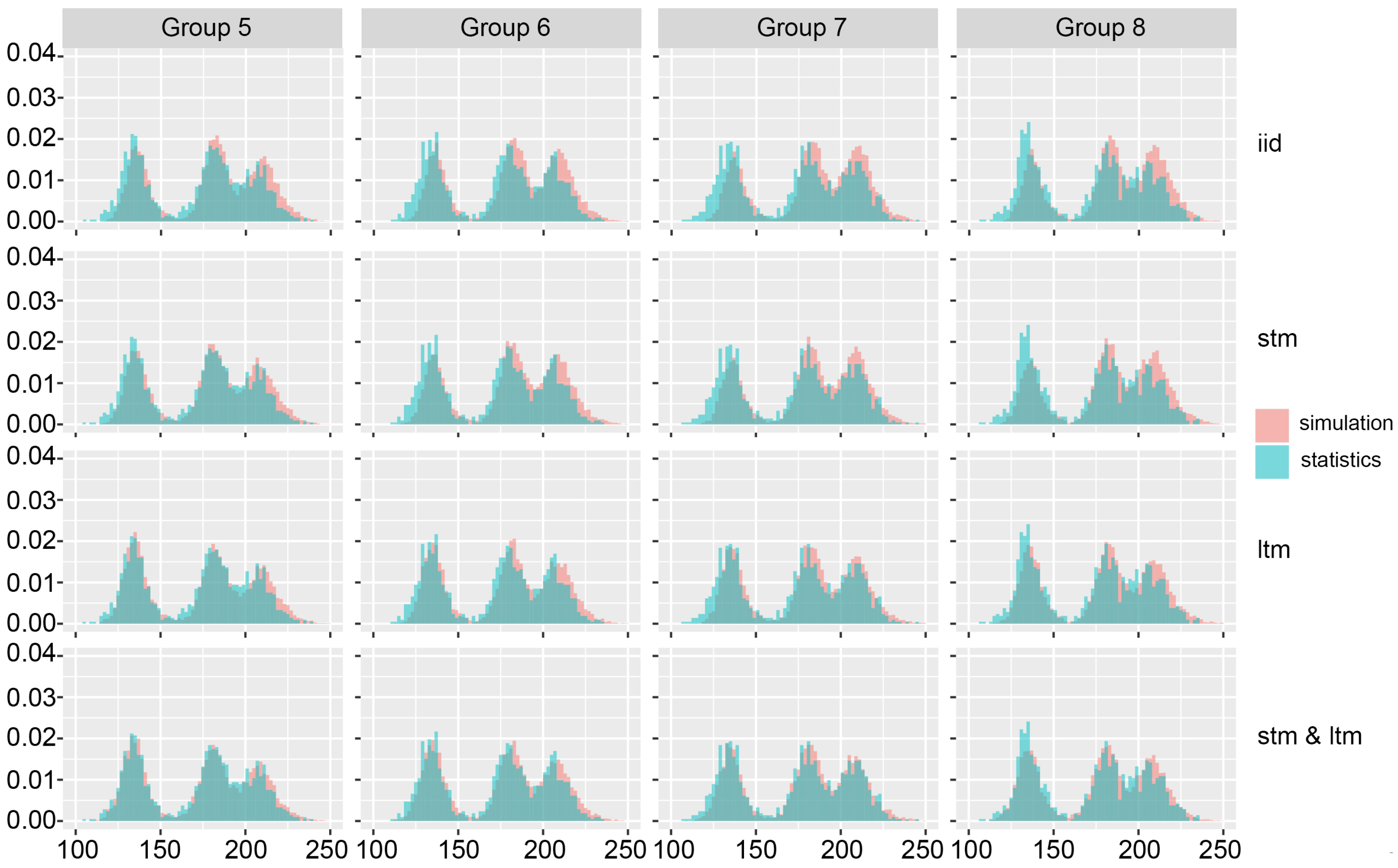
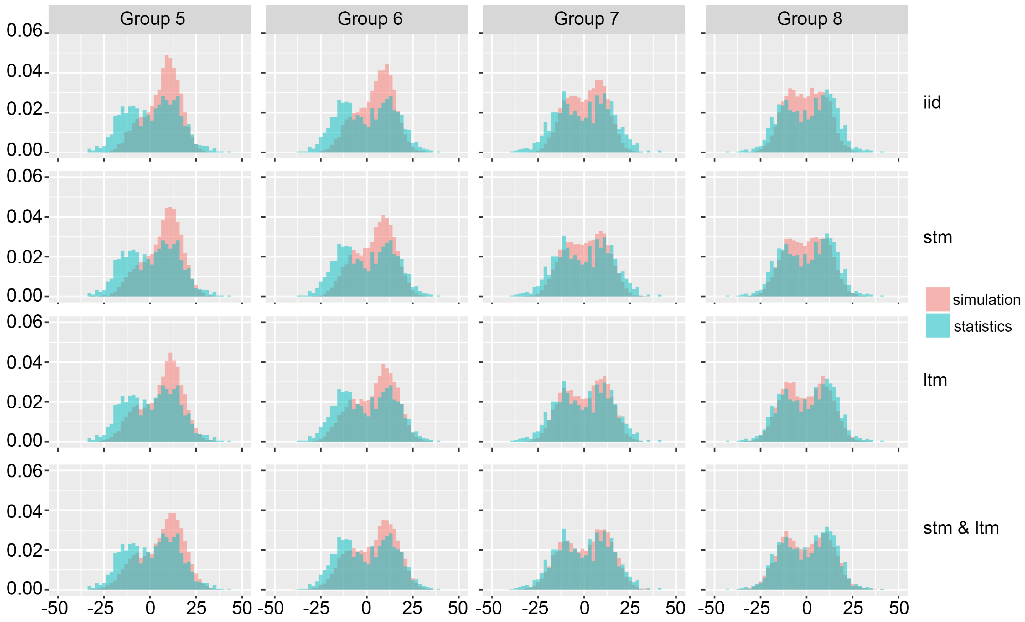
To present the results in a visually interpretable manner, overlapping total points/ handicap histograms for each group of matches are plotted. One histogram shows the real distribution of the total number of points played in a group of matches/handicap obtained from the real data, while the other represents the simulated total points/handicap distribution. A large overlapping area naturally represents closer adherence between simulated and real distributions. A two-level Euclidean distance measure (L2-norm) was used to numerically support the graphs.

The overlap was leveraged in the training process to optimize the parameters used by the evolving probability method. As stated earlier in this paper, the only parameters that need to be optimized are the parameters of the linear function, k and l, necessary for the calculation of the long-term momentum (all other parameters shown in Table 2 are calculated directly from the historical data). For the purpose of optimization, the traditional empirical algorithmic approach, grid search, was chosen. The optimal combination of parameters k and l is the combination that minimizes the simulation error of all groups, in both total points and handicap overlapping histograms. Due to the nature of the optimization problem a two-level L2-norm (Euclidean distance measure) was chosen to solve the problem. The norm representation is shown below in Equations (9)–(11). In order to find the optimal values for k and l, 70% of the entire dataset was used, leaving the rest for evaluation. The finally chosen values were $k=1.5$ and $l=250$:

$$E_{totalPts}=\sqrt{{\left(E_{totalPt{s}_1}\right)}^2+...+{\left(E_{totalPt{s}_8}\right)}^2}$$

(9)

$$E_{handicap}=\sqrt{{\left(E_{handica{p}_1}\right)}^2+...+{\left(E_{handica{p}_8}\right)}^2}$$

(10)

$$E=\sqrt{{\left(E_{totalPts}\right)}^2+{\left(E_{handicap}\right)}^2}$$

(11)

where:

$E_{totalPt{s}_i}$, i $ϵ$ [1,8]

—total points simulation error in a particular group;

$E_{handica{p}_i}$, i $ϵ$ [1,8]

—handicap simulation error in a particular group;

$E_{totalPts}$

—total simulation error in all total point histograms;

$E_{totalPts}$

$E_{handicap}$—total simulation error in all handicap histograms;

E 

—total simulation error.

After determining the optimal values of parameters k and l, the rest of the dataset was used to present the final results. Each match was placed in one of eight groups based on the pre-match betting odds. The corresponding group profile was used (except $p_{hist}$ and $q_{hist}$—they are calculated from the test set of data) to model the new match whose outcomes in terms of handicap and total points were to be predicted. Based on all matches of one group, the following histograms were created—see figures (Figure 5, Figure 6, Figure 7 and Figure 8). Figure 5 shows the overlapping total points distribution histograms for the first four groups of matches. The blue histograms show the real total points distribution for the corresponding group of matches, while the red ones show the simulated total points distribution. Each column of histograms on the figure represents one group, and each row refers to the aforementioned four different simulations. Similarly, Figure 6 shows the total points distribution for the last four groups of matches. Figure 7 shows the handicap distribution histograms for the first four groups of matches, while Figure 8 shows the handicap distribution histograms for the last four groups of matches.

By observing the first row of histograms in Figure 5, Figure 6, Figure 7 and Figure 8, it can be seen that by using the iid assumption results in a relatively large difference between the real distribution and the distribution obtained by the simulation. When the dynamics in the form of short-term and long-term sport momentums are introduced, the results are noticeably improved, as evidenced by a much larger overlap.

The graphical results are further supported by the numerical values shown in

Table 3. Total points simulation error.

Group	iid	stm	ltm	stm and ltm
1	0.4188	0.4457	0.3905	0.4338
2	0.4058	0.4328	0.3938	0.3999
3	0.4162	0.4321	0.3793	0.3844
4	0.4374	0.4282	0.3962	0.3763
5	0.3725	0.3326	0.3146	0.2943
6	0.4133	0.3938	0.3674	0.3452
7	0.4320	0.3929	0.3725	0.3165
8	0.4346	0.4115	0.3699	0.3342

and

Table 4. Handicap simulation error.

Group	iid	stm	ltm	stm and ltm
1	0.6383	0.6293	0.5970	0.5802
2	0.6203	0.6052	0.5649	0.5426
3	0.6210	0.6087	0.5631	0.5427
4	0.5775	0.5440	0.5095	0.4687
5	0.5095	0.4932	0.4494	0.4253
6	0.5155	0.4899	0.4362	0.4027
7	0.4514	0.4040	0.3583	0.3074
8	0.4287	0.3843	0.3450	0.2953

which show the total points simulation error (see Equations (9)–(11)) for each group of matches and the handicap simulation error for each group of matches, respectively.

Significant improvement is particularly evident in the last five groups of matches where the combination of short-term and long-term momentum gives the best results for predicting both total points and the handicap. In the first two groups of matches, using only the long-term momentum parameter shows better results when predicting the total number of points compared to the evolving probability method, which may support the hypothesis that the short-term momentum loses its impact when there is a significant difference in team strength ratios, so the stronger team can more easily start dominating the match. Nonetheless, it can be stated that using match dynamics consistently provides better results when compared with only using the iid-based simulation.

4. Discussion

In this paper, a common approach of modeling Markovian sports which relies on the assumption of identical and independent point distribution (iid) was challenged by introducing match dynamics in the form of short- and long-term sports momentums. Mathematical formulations for those two concepts were proposed and the influence of short-term and long-term sport momentums on the prediction of certain characteristics in volleyball matches was studied, most notably the total number of points that will be played in the matches and handicap. The method was tested on a real dataset and the results confirmed the initial assumption—by introducing dynamics into the simulation of volleyball matches, it is possible to more accurately simulate the real flow of a match and consequently obtain significantly better results when predicting the aforementioned characteristics of the volleyball match compared to the widely used iid assumption. Significant improvement is particularly evident in the last five groups of matches. When predicting the total number of points that will be played in those groups of matches, the simulation error when using the approach that combines short- and long-term sports momentums is on average 20% smaller compared to the iid approach. Even greater improvement is evident when using the evolving probability approach to predict the handicap. The simulation error, in this case, is on average 25% smaller compared to the iid approach. It is important to note that in the first two groups of matches, using only the long-term momentum parameter shows better results when predicting the total number of points compared to the evolving probability method. Such results were expected and they support the hypothesis that the short-term momentum loses its impact when there is a significant difference in team strength ratios.

It needs to be emphasized once again that the method proposed in this paper is an interpretable simulation method, and the method can very easily be incorporated into expert systems to gain insight into possible match score sequences that may arise under different circumstances. Experts in the sports domain can use the simulations to identify, understand and optimize player performance. The method is very flexible and can be easily upgraded by defining other parameters such as psychological pressure and fatigue.

A secondary part of this paper, but still necessary for the result demonstration, was the profiling part. Due to the limitations of the dataset used in this research, this paper proposes a profiling method that was adapted to work on heterogeneous datasets. In future work, a dataset that would have more information about the historical matches of each team will be collected. This will allow to focus on the profiling step, and to build much more detailed profiles at the team level rather than the match level. It would be interesting to explore how much it would contribute to the improvement of the results of the proposed predictive model.

The paper focuses on examining the assumption of independent point distribution. By introducing the short-term momentum formulation, the paper proved that the assumption of independent point distribution is not necessarily adequate when predicting different characteristics of a sports match—volleyball matches in particular. To examine the quality of the identical distribution of points in the prediction of certain characteristics of the volleyball match, in future work, the idea is to test the influence of the decisive points on the psychology of the team and embed this feature in the model proposed in this paper. The future research will also focus on applying the proposed model to other discrete sports, especially tennis, which is usually a sport of particular interest in sports data mining.