
Complex Network Modelling of Origin–Destination Commuting Flows for the COVID-19 Epidemic Spread Analysis in Italian Lombardy Region

 ,
,  ,
,  ,
,  and
and 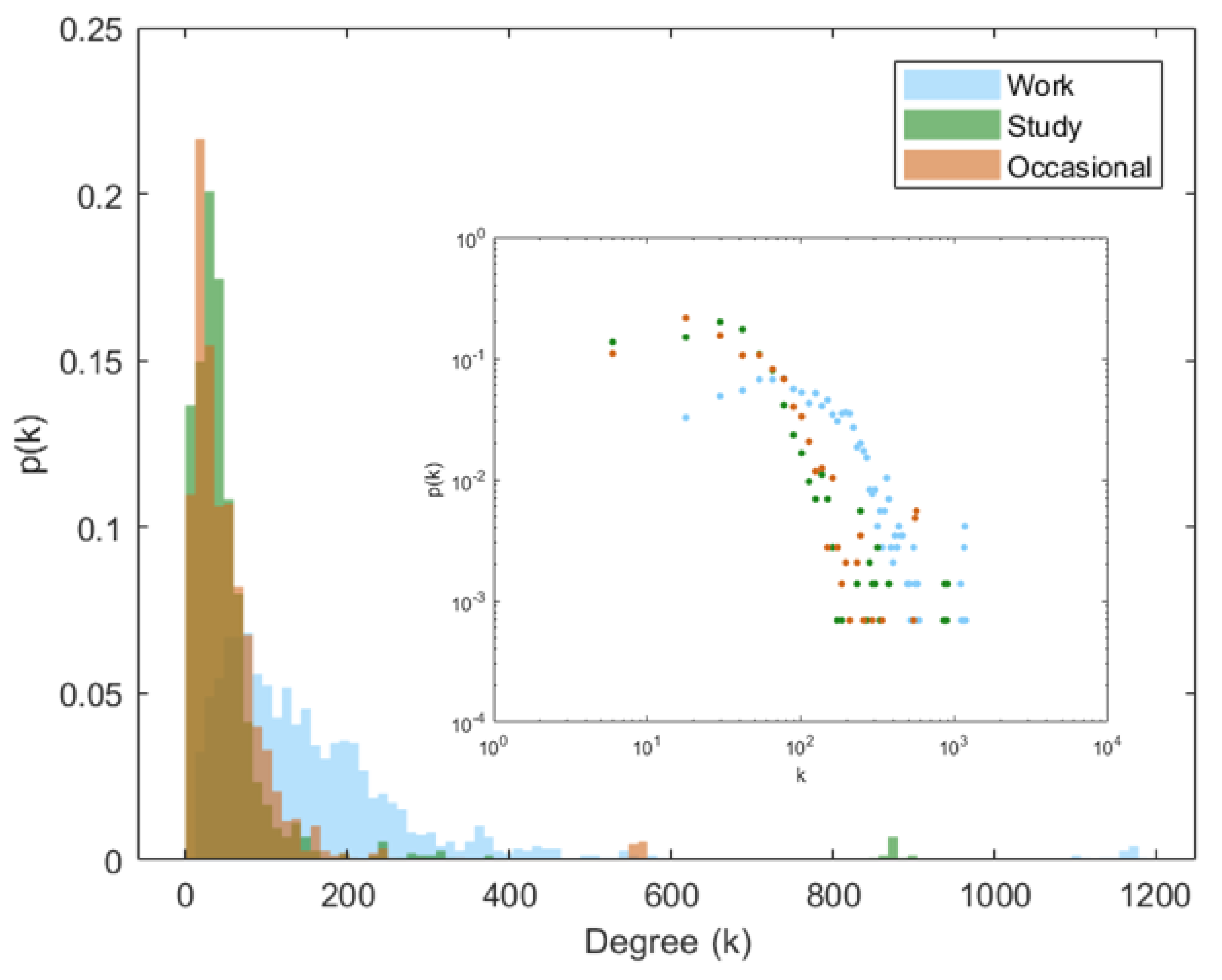
Abstract
1. Introduction
2. Materials and Methods
2.1. Origin–Destination Networks
2.2. Epidemic Spread on Networks
- transmission from an infected node to a susceptible node occurs across an edge as a Poisson process with rate ;
- an infected node recovers by following a Poisson process with rate .
2.3. Statistical Analysis
- value of the peak;
- time at which the peak occurs;
- area under the curve.
3. Results
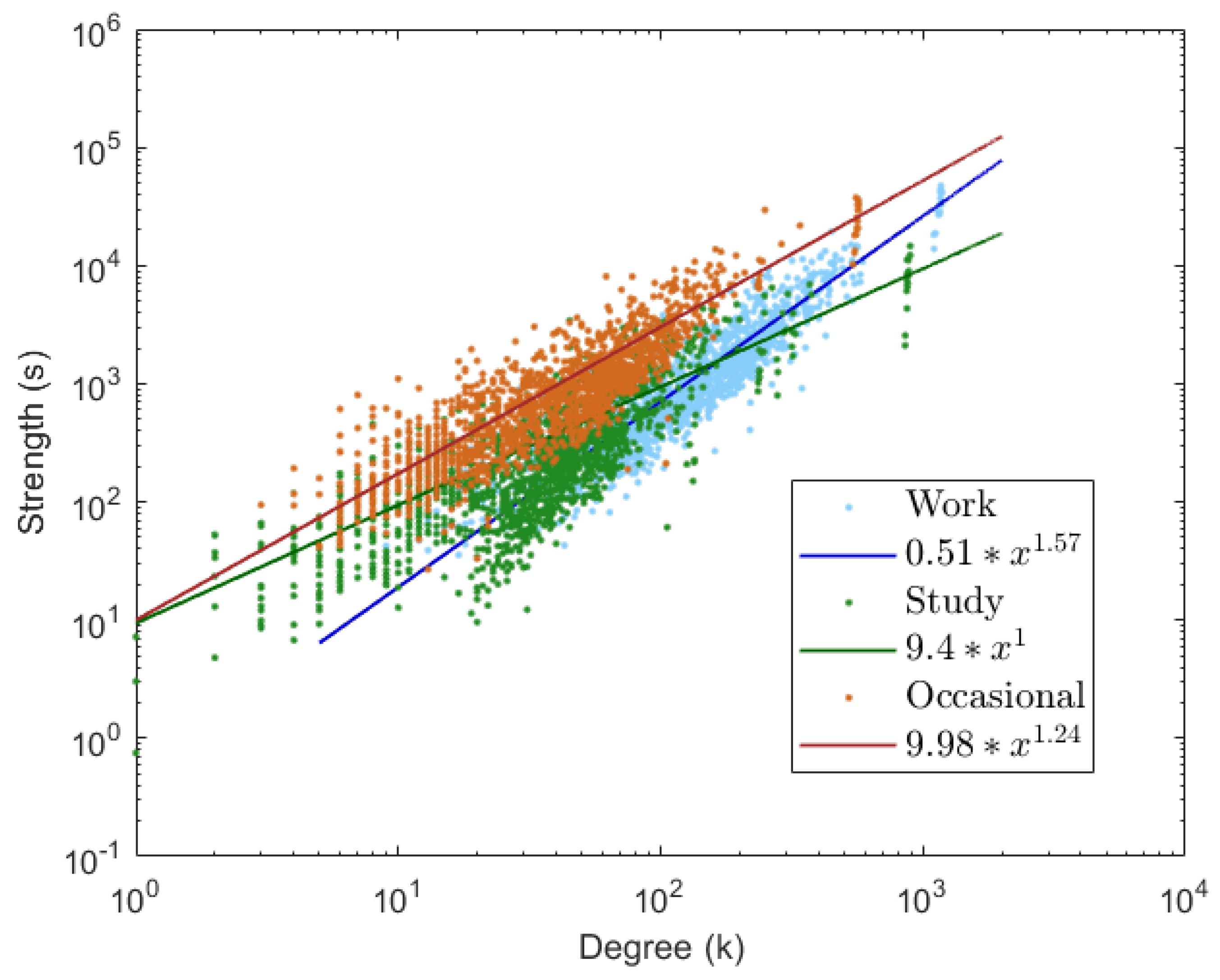
3.1. Network Structure
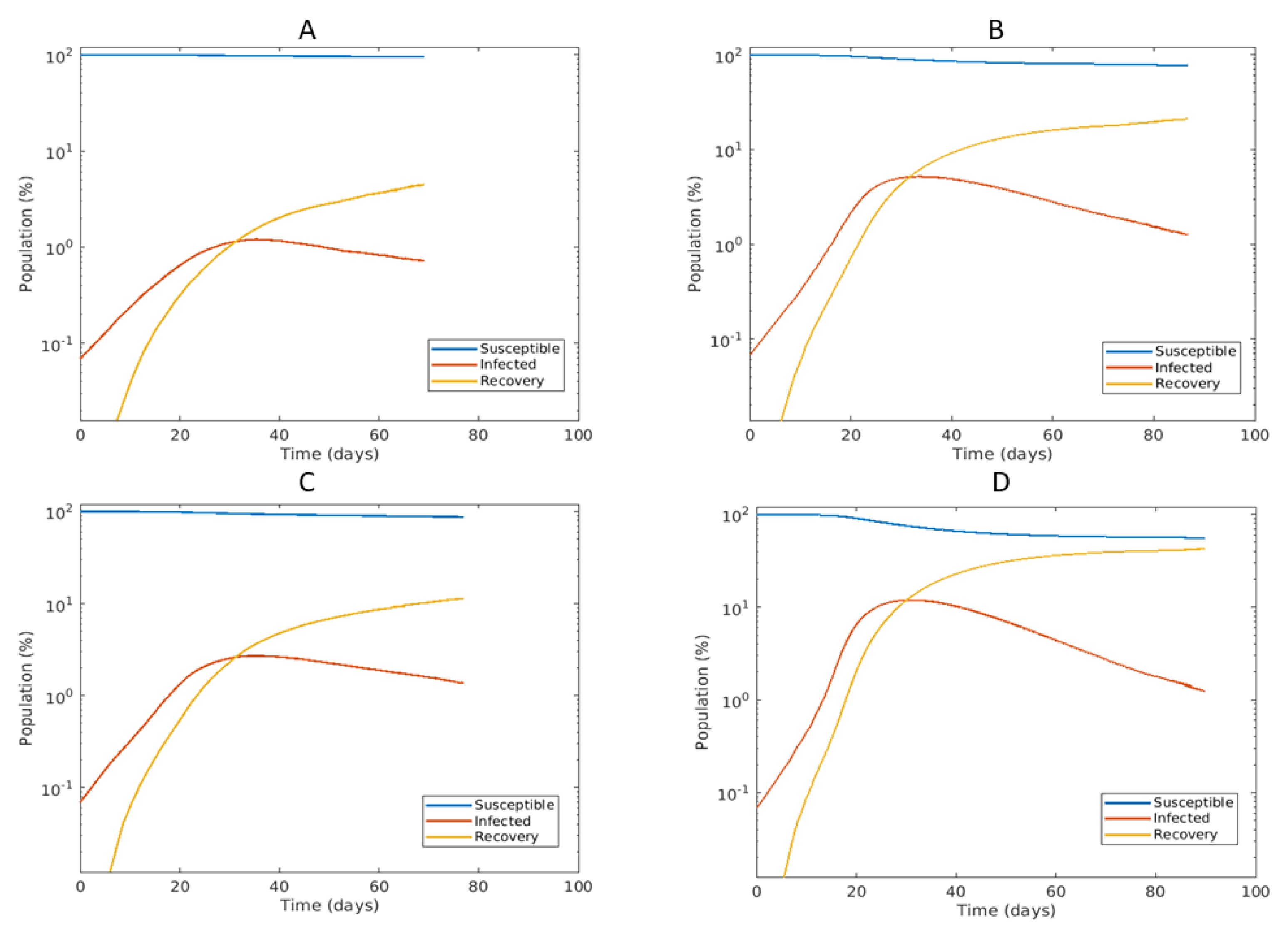
3.2. Simulations of Epidemic Spread
4. Discussion
5. Conclusions
Author Contributions
Funding
Conflicts of Interest
References
- Paules, C.I.; Marston, H.D.; Fauci, A.S. Coronavirus infections—More than just the common cold. JAMA 2020, 323, 707–708. [Google Scholar] [CrossRef]
- World Health Organization. Coronavirus Disease 2019 (COVID-19): Situation Report, 82; World Health Organization: Geneva, Switzerland, 2020. [Google Scholar]
- World Health Organization. WHO Director-General’s Opening Remarks at the Media Briefing on COVID19- March 2020; World Health Organization: Geneva, Switzerland, 2020. [Google Scholar]
- Available online: https://coronavirus.jhu.edu/map.html (accessed on 7 April 2021).
- Report45, Monitoraggio Fase2 (DM Salute 20 Aprile 2020), Dati Relativi alla Settimana 15/3/2021–21/3/2021; Ministero della Salute, Istituto Superiore di Sanitá, Cabina di Regia ai sensi del DM Salute: Rome, Italy, 2020.
- Pastor-Satorras, R.; Castellano, C.; Van Mieghem, P.; Vespignani, A. Epidemic processes in complex networks. Rev. Mod. Phys. 2015, 87, 925. [Google Scholar] [CrossRef]
- Colizza, V.; Barrat, A.; Barthélemy, M.; Vespignani, A. The role of the airline transportation network in the prediction and predictability of global epidemics. Proc. Natl. Acad. Sci. USA 2006, 103, 2015–2020. [Google Scholar] [CrossRef]
- Colizza, V.; Barrat, A.; Barthélemy, M.; Vespignani, A. The modeling of global epidemics: Stochastic dynamics and predictability. Bull. Math. Biol. 2006, 68, 1893–1921. [Google Scholar] [CrossRef]
- Ni, S.; Weng, W. Impact of travel patterns on epidemic dynamics in heterogeneous spatial metapopulation networks. Phys. Rev. E 2009, 79, 016111. [Google Scholar] [CrossRef]
- Nouvellet, P.; Bhatia, S.; Cori, A.; Ainslie, K.E.; Baguelin, M.; Bhatt, S.; Boonyasiri, A.; Brazeau, N.F.; Cattarino, L.; Cooper, L.V.; et al. Reduction in mobility and COVID-19 transmission. Nat. Commun. 2021, 12, 1–9. [Google Scholar] [CrossRef] [PubMed]
- Colizza, V.; Barrat, A.; Barthelemy, M.; Valleron, A.J.; Vespignani, A. Modeling the worldwide spread of pandemic influenza: Baseline case and containment interventions. PLoS Med. 2007, 4, e13. [Google Scholar] [CrossRef]
- Bowen, J.T., Jr.; Laroe, C. Airline networks and the international diffusion of severe acute respiratory syndrome (SARS). Geogr. J. 2006, 172, 130–144. [Google Scholar] [CrossRef]
- Chinazzi, M.; Davis, J.T.; Ajelli, M.; Gioannini, C.; Litvinova, M.; Merler, S.; Y Piontti, A.P.; Mu, K.; Rossi, L.; Sun, K.; et al. The effect of travel restrictions on the spread of the 2019 novel coronavirus (COVID-19) outbreak. Science 2020, 368, 395–400. [Google Scholar] [CrossRef] [PubMed]
- Amini, B.; Peiravian, F.; Mojarradi, M.; Derrible, S. Comparative analysis of traffic performance of urban transportation systems. Transp. Res. Rec. 2016, 2594, 159–168. [Google Scholar] [CrossRef]
- Tak, S.; Kim, S.; Byon, Y.J.; Lee, D.; Yeo, H. Measuring health of highway network configuration against dynamic Origin–Destination demand network using weighted complex network analysis. PLoS ONE 2018, 13, e0206538. [Google Scholar] [CrossRef] [PubMed]
- Newman, M.E. The structure and function of complex networks. SIAM Rev. 2003, 45, 167–256. [Google Scholar] [CrossRef]
- Boccaletti, S.; Latora, V.; Moreno, Y.; Chavez, M.; Hwang, D.U. Complex networks: Structure and dynamics. Phys. Rep. 2006, 424, 175–308. [Google Scholar] [CrossRef]
- Barrat, A.; Barthelemy, M.; Pastor-Satorras, R.; Vespignani, A. The architecture of complex weighted networks. Proc. Natl. Acad. Sci. USA 2004, 101, 3747–3752. [Google Scholar] [CrossRef]
- Anderson, R.M.; Anderson, B.; May, R.M. Infectious Diseases of Humans: Dynamics and Control; Oxford University Press: Oxford, UK, 1992. [Google Scholar]
- Koziol, K.; Stanislawski, R.; Bialic, G. Fractional-Order SIR Epidemic Model for Transmission Prediction of COVID-19 Disease. Appl. Sci. 2020, 10, 8316. [Google Scholar] [CrossRef]
- Kiss, I.Z.; Miller, J.C.; Simon, P.L. Mathematics of Epidemics on Networks; Springer: Cham, Switzerland, 2017; Volume 598. [Google Scholar]
- Atkeson, A. What Will Be the Economic Impact of COVID-19 in the US? Rough Estimates of Disease Scenarios; Technical Report; National Bureau of Economic Research: Cambridge, MA USA, 2020. [Google Scholar]
- Remuzzi, A.; Remuzzi, G. COVID-19 and Italy: What next? Lancet 2020, 395, 1225–1228. [Google Scholar] [CrossRef]
- Anderson, R.M.; Heesterbeek, H.; Klinkenberg, D.; Hollingsworth, T.D. How will country-based mitigation measures influence the course of the COVID-19 epidemic? Lancet 2020, 395, 931–934. [Google Scholar] [CrossRef]
- Guimera, R.; Mossa, S.; Turtschi, A.; Amaral, L.N. The worldwide air transportation network: Anomalous centrality, community structure, and cities’ global roles. Proc. Natl. Acad. Sci. USA 2005, 102, 7794–7799. [Google Scholar] [CrossRef]
- Barabási, A.L. Scale-free networks: A decade and beyond. Science 2009, 325, 412–413. [Google Scholar] [CrossRef]
- La Gatta, V.; Moscato, V.; Postiglione, M.; Sperli, G. An Epidemiological Neural network exploiting Dynamic Graph Structured Data applied to the COVID-19 outbreak. IEEE Trans. Big Data 2020. [Google Scholar] [CrossRef]
- Hâncean, M.G.; Slavinec, M.; Perc, M. The impact of human mobility networks on the global spread of COVID-19. J. Complex Netw. 2020, 8, cnaa041. [Google Scholar] [CrossRef]
- Dehning, J.; Zierenberg, J.; Spitzner, F.P.; Wibral, M.; Neto, J.P.; Wilczek, M.; Priesemann, V. Inferring change points in the spread of COVID-19 reveals the effectiveness of interventions. Science 2020, 369. [Google Scholar] [CrossRef]
- Zhong, L.; Mu, L.; Li, J.; Wang, J.; Yin, Z.; Liu, D. Early prediction of the 2019 novel coronavirus outbreak in the mainland China based on simple mathematical model. IEEE Access 2020, 8, 51761–51769. [Google Scholar] [CrossRef] [PubMed]
- Liu, M.; Thomadsen, R.; Yao, S. Forecasting the spread of COVID-19 under different reopening strategies. Sci. Rep. 2020, 10, 1–8. [Google Scholar] [CrossRef]
- Gatto, M.; Bertuzzo, E.; Mari, L.; Miccoli, S.; Carraro, L.; Casagrandi, R.; Rinaldo, A. Spread and dynamics of the COVID-19 epidemic in Italy: Effects of emergency containment measures. Proc. Natl. Acad. Sci. USA 2020, 117, 10484–10491. [Google Scholar] [CrossRef] [PubMed]


Publisher’s Note: MDPI stays neutral with regard to jurisdictional claims in published maps and institutional affiliations. |
© 2021 by the authors. Licensee MDPI, Basel, Switzerland. This article is an open access article distributed under the terms and conditions of the Creative Commons Attribution (CC BY) license (https://creativecommons.org/licenses/by/4.0/).
Share and Cite
Lombardi, A.; Amoroso, N.; Monaco, A.; Tangaro, S.; Bellotti, R. Complex Network Modelling of Origin–Destination Commuting Flows for the COVID-19 Epidemic Spread Analysis in Italian Lombardy Region. Appl. Sci. 2021, 11, 4381. https://doi.org/10.3390/app11104381
Lombardi A, Amoroso N, Monaco A, Tangaro S, Bellotti R. Complex Network Modelling of Origin–Destination Commuting Flows for the COVID-19 Epidemic Spread Analysis in Italian Lombardy Region. Applied Sciences. 2021; 11(10):4381. https://doi.org/10.3390/app11104381
Chicago/Turabian StyleLombardi, Angela, Nicola Amoroso, Alfonso Monaco, Sabina Tangaro, and Roberto Bellotti. 2021. "Complex Network Modelling of Origin–Destination Commuting Flows for the COVID-19 Epidemic Spread Analysis in Italian Lombardy Region" Applied Sciences 11, no. 10: 4381. https://doi.org/10.3390/app11104381
APA StyleLombardi, A., Amoroso, N., Monaco, A., Tangaro, S., & Bellotti, R. (2021). Complex Network Modelling of Origin–Destination Commuting Flows for the COVID-19 Epidemic Spread Analysis in Italian Lombardy Region. Applied Sciences, 11(10), 4381. https://doi.org/10.3390/app11104381