Article

Health Monitoring of Stress-Laminated Timber Bridges Assisted by a Hygro-Thermal Model for Wood Material

1
VTT Technical Research Centre of Finland Ltd., P.O. Box 1000, VTT, 02044 Espoo, Finland
2
Standards Norway, P.O. Box 242, NO-1326 Lysaker, Norway
3
Väylävirasto, Opastinsilta 12 A, 00520 Helsinki, Finland
*
Author to whom correspondence should be addressed.
Appl. Sci. 2021, 11(1), 98; https://doi.org/10.3390/app11010098
Submission received: 29 November 2020 / Revised: 17 December 2020 / Accepted: 22 December 2020 / Published: 24 December 2020

Abstract

:
Timber bridges are economical, easy to construct, use renewable material and can have a long service life, especially in Nordic climates. Nevertheless, durability of timber bridges has been a concern of designers and structural engineers because most of their load-carrying members are exposed to the external climate. In combination with certain temperatures, the moisture content (MC) accumulated in wood for long periods may cause conditions suitable for timber biodegradation. In addition, moisture induced cracks and deformations are often found in timber decks. This study shows how the long term monitoring of stress-laminated timber decks can be assisted by a recent multi-phase finite element model predicting the distribution of MC, relative humidity (RH) and temperature (T) in wood. The hygro-thermal monitoring data are collected from an earlier study of the Sørliveien Bridge in Norway and from a research on the new Tapiola Bridge in Finland. In both cases, the monitoring uses integrated humidity-temperature sensors which provide the RH and T in given locations of the deck. The numerical results show a good agreement with the measurements and allow analysing the MCs at the bottom of the decks that could be responsible of cracks and cupping deformations.

1. Introduction

Timber and engineered wood have increased their popularity as structural materials thank to their outstanding environmental performance, competitive price, mechanical properties, and relatively easy handling. However, the use of wood in unsheltered bridges is rather limited because of the exposure to the harsh climate conditions. Designers and structural engineers are mostly worried about the service life of the load-carrying structures which is recommended to be one hundred years in Europe [1].
Although evidence exists that structural wood can retain its strength through many centuries [2], it is very sensitive to the variable temperature (T) and moisture content (MC) which may lead to the material degradation and loss of its structural performance [3]. In some cases, the biotic damage can grow from inside out, and therefore the proper monitoring of internal material condition is essential in wooden bridges.
Stress-laminated timber decks (SLTDs) are composed of wood lamellas placed longitudinally between the supports of the bridge and compressed together with preloaded steel bars in the transverse direction (see [4] and the related references). This technology was developed in Canada in 1976 to replace nail-laminated wooden decks, which delaminated under cyclic loading and moisture variation. The first stress-laminated bridges were built in North America in 1980. The technology was adapted in Europe in mid 1980s and it was introduced in Australia, Japan and other countries since 1990. The greatest advantage of laminated decks is that they form a stiff and solid base for the pavement, and therefore can redistribute the external loads to their supports. This effect is due to the prestressing action of the high-strength steel bars that squeeze the wooden lamellas together. The bar force, measured by using load cells, is typically from 89 to 356 kN [4].
Even though many of the originally built stress-laminated decks are performing well over three decades, it is essential to avoid errors during the construction and maintenance of the bridge. For instance, Scharmacher et al. [5] reported that blistering between wood and asphalt surface may occur, because of high MC of the deck and elevated asphalt temperature. This will affect the performance of the shear connection, but may also create conditions for water accumulation or ice formation under the asphalt surface.
Since the stress-laminating technology was developed in Canada and the northern parts of the United States, the effect of freezing temperatures has been thoroughly examined [4]. Laboratory tests revealed significant decrease of the bar forces of deck sections placed from a temperature of 21.1 °C to temperatures below zero ranging between −12.2 °C and −34.4 °C, strongly depending on the MC of the wood. Therefore, Wacker [4] recommends thermal design considerations in cold climates such as Alaska and Canada. This recommendation should also be applicable to the Nordic countries with similar weather conditions. Apparently, the simplest thermal design consideration is to keep the MC low in winter months to prevent the loss of pre-loading forces in the high-strength steel bars.
During the last decades, the development of timber bridges in European Nordic countries has been promoted by the joint effort of road authorities, timber industries and research organizations. A result of this cooperation was the Nordic Timber Bridges Programme [6]. Part of the activities under this programme was monitoring the long-term behaviour of wooden bridges in Norway financed by the Norwegian Public Roads Administration. Five of the monitored bridges in Norway have SLTDs and are located in Evenstad, Daleråsen, Flisa, Sørliveien and Måsør [7]. The bridges are built between 1996 and 2005 and are typically multi-span structures with glue laminated arches or trusses as the main load-carrying system. All of them have similar deck composed of 48 × 233 mm lamellas treated with creosote excepting the footbridge in Sørliveien (Figure 1), which has a deck of untreated spruce and a deck height of 333 mm, made of vertically sawn glulam beams. The SLT deck protecting the whole bridge structure is shown for Sørliveien Bridge (Norway) in Figure 1a. In addition, Figure 1b shows a detail of the SLT deck with the view of the wood lamellas and the steel bars for the same bridge.
The efforts to promote timber bridges continued also after the end of Nordic Timber Bridges Programme. For instance, the Wood Building Programme (2016–2021) was launched in Finland as a government undertaking to increase the use of wood in urban development, public buildings, bridges and halls [8]. The programme is also seen as an efficient way of attaining the energy and climate targets to reduce Finland’s carbon footprint by 2030. However, the number of laminated wooden deck bridges for vehicle traffic in Finland is still relatively small. One such bridge, carrying significant vehicle traffic, is the highway crossing recently erected in the Tapiola district of the city of Espoo. The Tapiola Bridge is now being permanently monitored under the supervision of the Finnish Transport Infrastructure Agency.
In addition to the durability problems, a common effect of moisture variation in SLTDs is the cupping deformation, which is usually measured as the uplift at the corner in the bottom surface of the deck [9]. A sharp increase of cupping is usually observed during wetting and only a partial decrease during drying. For the details, the reader is referred to Section 4.3 of the Durable Timber Bridges report [9].
The above review about performance of bridges shows that control of the MC in wooden parts is not only essential for the durability of the material, but for the whole superstructure as well. Variation of the MC directly affects structural integrity, serviceability and loading capacity of the bridge. Therefore, the monitoring techniques have a fundamental role in controlling the health of large structures exposed to outdoor climates, such as timber bridges. However, measurements obtained by the usual monitoring techniques based, e.g., on integrated humidity-temperature sensors, provide hygro-thermal measurements only in specific locations of the wood components.
As shown in the recent literature [10,11,12], advanced multi-phase models are an effective tool to assist the hygro-thermal monitoring of timber bridge components such as glulam beams. Compared to the single-phase (or single-Fickian) models for transient moisture transport in wood [13,14,15], where the MC is the only variable of a Fick’s second law equation, the multi-phase models below the fibre saturation point (FSP) analyse two different water phases, i.e., the water vapour in lumens and the bound water in wood-cell walls. Starting from the seminal works of Krabbenhøft [16] and Frandsen [17], there was a strong effort to develop a multi-phase theory (often called multi-Fickian) for moisture transport in wood that includes the conversion rates between the different water phases. The multi-Fickian theory below the FSP is based on the identification of three phenomena occurring in cellular wood during moisture transfer, i.e., the diffusion of water vapour in the lumens, the sorption of bound water and the diffusion of bound water in the cell walls. In the multi-phase models available in the current literature, the two water phases are separated and the coupling between them is defined through a sorption rate [10,11,12,17,18,19,20]. Recently, Autengruber et al. [21], developed a whole multi-Fickian model including also the transport of free water in the lumens above the FSP. Therefore, in addition to the sorption rate between the two phases of water vapour and bound water, also the sorption rate between the free water and bound water phases, as well as the evaporation/condensation rate between the free water and the water vapour phases, need to be defined. These phenomena are schematized in Figure 2. For a complete description of the moisture transfer in wood, a sorption hysteresis characterized by two isotherms of adsorption and desorption was originally introduced in the multi-Fickian model by Frandsen [17]. In the present work, only case-studies with moisture states below the FSP are studied.
As discussed by Svensson et al. [22] and Fragiacomo et al. [13], high values of moisture gradients due to high yearly and daily variations of relative humidities are the main causes of moisture induced stresses (MIS) perpendicular to the grains in wooden members. Larger yearly variations of RH (average values above 80%) and larger moisture gradients and MIS in timber cross sections were found under Northern European climates when compared to Southern European climates [13]. In [10,11] it was observed that, under Norther climates, high gradients in the vicinity of surfaces of bridge glulam beams during drying periods of the year are caused by high peaks of RH (above 85%) in conjunction with high daily variations of RH (above 50%). Knowledge on moisture gradients is therefore important to identify the zones prone to crack risk in wooden components, as shown in [12] for the case of a bridge glulam beam where the MIS were also calculated and discussed in relation to the moisture gradients. In [12] it was found that the most critical MIS are the tensile stresses perpendicular to the grain that can be also greater than the limits prescribed by the Eurocodes. Due to this, the uncoated bridge wooden beams may be exposed to the formation of moisture induced cracks and delamination. The structural significance of cracks in timber bridges under outdoor environments is discussed also in [23] where the asymmetric damage (longitudinal splitting cracks) is especially investigated.
Models for moisture transport, coupled with mechanical models, can be used to calculate the moisture induced cupping in stress laminated timber decks. The models can also allow the evaluation of the bar force losses during time, as shown in Section 4 of [9], were a single-phase model for moisture transport was used.
The novelty of the present paper is the use of a recent multi-phase model, proposed by some of the authors in [11], to assist the monitoring of SLTDs of bridges under Nordic European climates carried out by integrated humidity-temperature sensors. In particular, the hygro-thermal monitored data are collected from a previous study of the untreated deck of Sørliveien Bridge in Norway [24,25] and from the on-going monitoring of the painted and thick deck of Tapiola Bridge in the city of Espoo, Finland. Untreated and painted bridges are interesting cases to study in terms of their hygro-thermal performance. In this paper, the monitoring systems of the Sørliveien and Tapiola bridges are presented, and selected measurements are used for simulation by the finite element method (FEM). While the monitoring provides the RH and T in some locations of the analysed decks, the numerical model completes the health monitoring providing the overall hygro-thermal response of a representative volume of the deck in terms of distribution of MC, vapour pressure and T. In particular, the hygro-thermal response of the bottom deck, which is more affected by the external climate, is investigated.

2. Materials and Methods

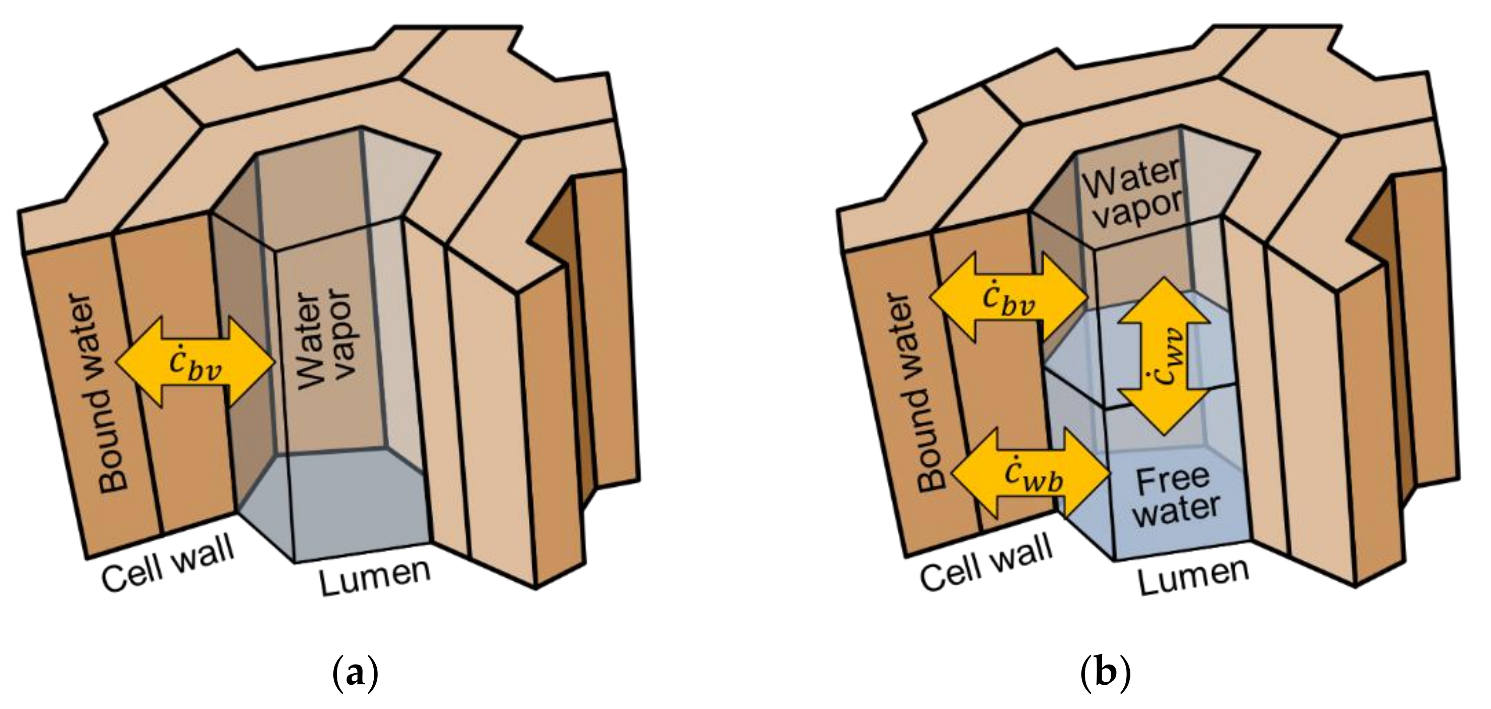
2.1. Description of the Multi-Phase Model

Summarizing the multi-Fickian model presented in [11] for wood below the FSP, the variables for transient moisture transport are the concentration of bound water in the cell walls c b , the concentration of water vapour in the cell lumens c v , and the temperature T . Denoting by D b and D v the diffusion tensors for bound water and water vapour phases and by K the thermal conductivity tensor, the governing equations of the problem are:
c b t =   · J b + c ˙ b v
c v t =   · J v   c ˙ b v
c w ϱ T t =   · J H   · J b h b   · J v h v +   c ˙ b v h b v
where is the nabla operator, J b and J v are the fluxes of bound water and water vapour, and J H represents the thermal flux:
J b = D b c b J v = D v c v , J H = K T
In Equation (3), c w represents the specific heat and ϱ the wood density, the coupling term c ˙ b v is the sorption rate between the two water phases (see Figure 1), h b and h v are the specific enthalpies and h b v = h b h v is the specific enthalpy of the transition from the bound water to the water vapour. The moisture content MC is defined as c b / ϱ 0 where ϱ 0 is the dry wood density. The sorption rate in Equations (1)–(3) is defined as:
c ˙ b v =   H c ϱ 0 M C b l c b
where H c represents the moisture dependent reaction rate and M C b l is the moisture content in equilibrium with the relative humidity. In Equation (5), the M C b l has the meaning of temperature-dependent sorption isotherms. These are defined by using the Anderson–McCarthy model (see Appendix A). In the present work, according to [11], an average between the temperature dependent adsorption and desorption isotherms is used, while a model for sorption hysteresis is not included.
Since the bound water cannot pass the external surfaces and it is restricted in the cell walls, the model includes only exchanges of vapour and heat with the ambient air. Therefore, the first boundary condition of Equation (6) holds on all the external surfaces in relation to variable c b . For the other variables, the second and third boundary conditions in Equation (6) apply for the external surfaces exposed to the variable RH and T:
n · J b = 0 , n · J v =   k v w   c v   k v a c v a , n · J v =   k T T   T a
where n represents the outward normal direction to the surface, c v a and T a are the water vapour concentration and temperature of the air, k v w and k v a the surface permeances corresponding to wood temperature and air temperature, and k T is the thermal emission coefficient. The expressions of the permeances are reported in Appendix A. In Equation (6), c v = c v / φ represents the concentration of water vapour divided by the wood porosity φ . The concentration c v is related to the partial vapour pressure p v through the ideal gas law:
c v = φ   p v M H 2 O / R T
where R is the gas constant and M H 2 O the molecular mass of water. The vapour pressure can be expressed as a function of the relative humidity R H :
p v = R H   · p v s
where p v s is the saturated vapour pressure given by the semi-empirical Kirchhoff expression for the thermal ranges above the freezing point and by Teten’s fitting for ice in the subfreezing temperature range [26]:
p v s = e x p 53.421 6516.3 T 4.125   ln T for   T 0 ° C 100 × 10 9.5 T 273.15 T 7.65 + 0.7858 for   T < 0 ° C
All material parameters of the model are summarized in Table A1 of Appendix A. The model is suitable for wooden members sheltered from rain and without water traps or other contacts with water. It does not allow the modelling of liquid water in pores and can simulate only moisture states below the FSP.

2.2. Implementation of the Hygro-Thermal Model for Stress-Laminated Timber Deck in Abaqus Code

The selected commercial finite element software Abaqus provides a comfortable environment for the 3D model construction and the evaluation of results. The finite element to be used for the hygro-thermal analysis was defined in the user subroutine UEL to accommodate the three differential equations that describe the material model. The subroutine is reading the weather data from the database of measured temperatures and air relative humidities at every time increment and applies them as external loads on the exposed model surfaces. The shape functions for 8-nodes isoparametric brick elements are used and a weak form of the governing equations and their boundary conditions with three variables per node (bound water concentration, water vapour concentration and temperature) is implemented in the UEL.
The time integration is carried out using the fully implicit Euler scheme and the nonlinear system is solved using the Newton method at each time step. The subroutine allows to implement the FEM contributions to the residual vector and to the Jacobian iteration matrix.
The general scheme for the hygro-thermal modelling of the timber deck is shown in Figure 3 and the simplifications used are the following:
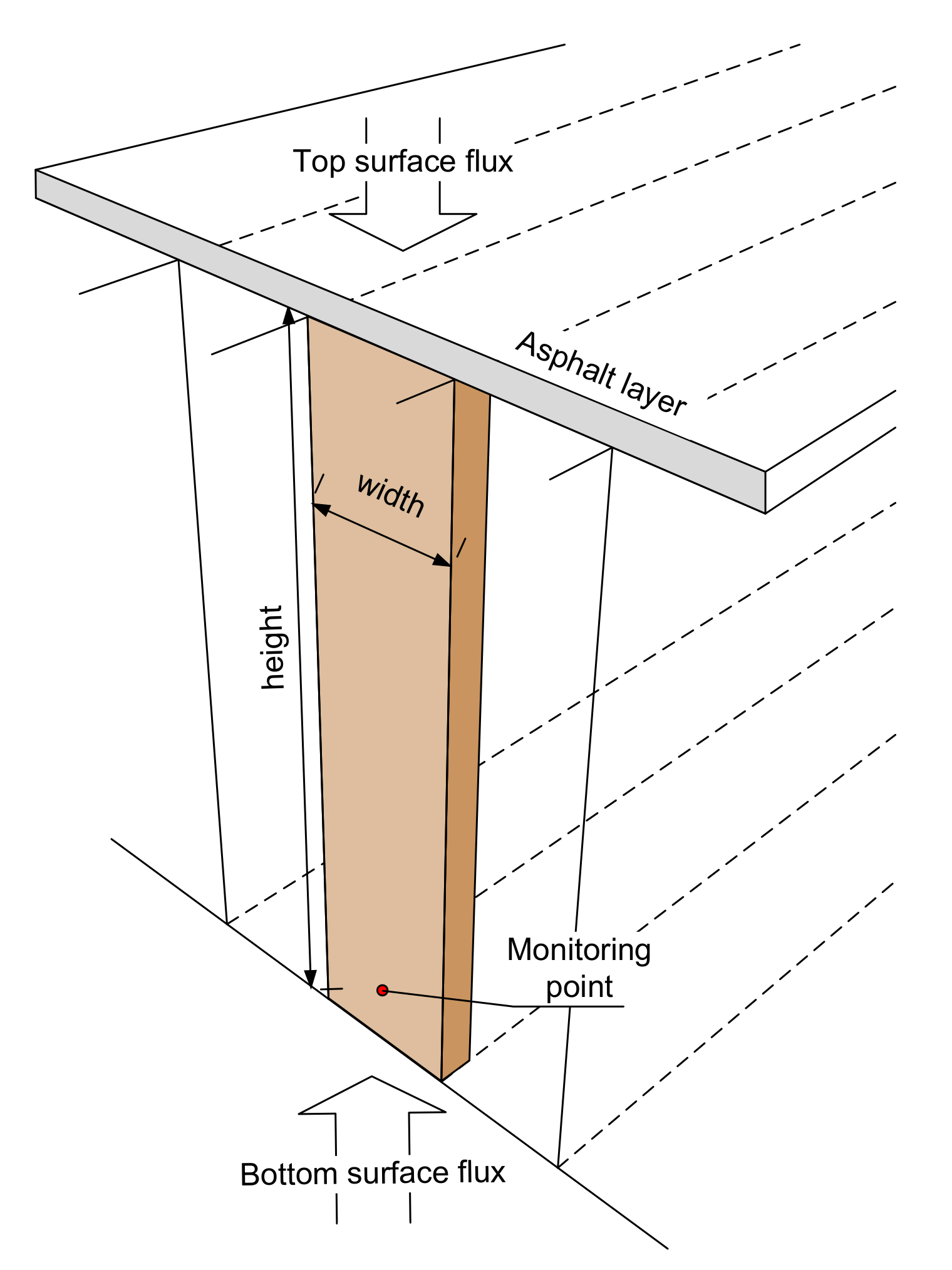
  • The model is a 3D slice of the deck far from the ends. The bottom face is exposed to the humidity and temperature of the air. The top surface is exposed only to temperature, because the top of the deck is protected from moisture by the asphalt layer.
  • The asphalt layer is not modelled.
  • The lateral, back and front faces are internal surfaces and therefore are not exposed to the air temperature or moisture fluxes.
  • The bottom surface is sheltered from rain and without water traps.
  • The model does not include the effect of solar radiation.
  • The height of the model represents the thickness of the timber deck and its width varies depending on the width of the lamella, with the mesh size of the FEM typically between 5 and 10 mm.
  • The effect of glue between lamellas is not considered.
The initial values for the variables of the differential problem are the following:
  • The temperature T 0 is chosen equal to the air temperature at the beginning of the analysis.
  • The concentration of bound water is calculated as c b 0 = ϱ 0 M C 0 , where M C 0 is the moisture content in equilibrium with the initial air relative humidity R H 0 at the beginning of the monitoring. This is obtained from the temperature dependent sorption isotherm listed in Table A2 of Appendix A.
  • The concentration of water vapour c v 0 is calculated by using Equations (7)–(9) and the R H 0 and T 0 .
The fluxes acting on the 3D slice of the deck are as follows:
  • The first boundary condition of Equation (6) applies on the top and bottom surfaces.
  • The heat flux and thermal flux act on the bottom surface exposed to the air temperature and relative humidity.
  • Only the heat flux acts on the top protected by the asphalt.
  • There are no fluxes on the lateral (internal) surfaces.
The input material data used for both case-studies of the paper are the dry wood density ϱ 0 = 450 kg/m3, the porosity φ = 0.65 and the coefficients of the diffusion tensors that are listed in Appendix A. The permeances for the uncoated wood used in the first case-study ( k w ) and for the weak paint used in the second case-study ( k p ) are listed in Table A3, and the thermal emission coefficient are listed in Table A1 of Appendix A.
The outputs are the moisture content MC, the vapour pressure p v (obtained from the water vapour concentration c v ), and the temperature T in each element of the 3D model.

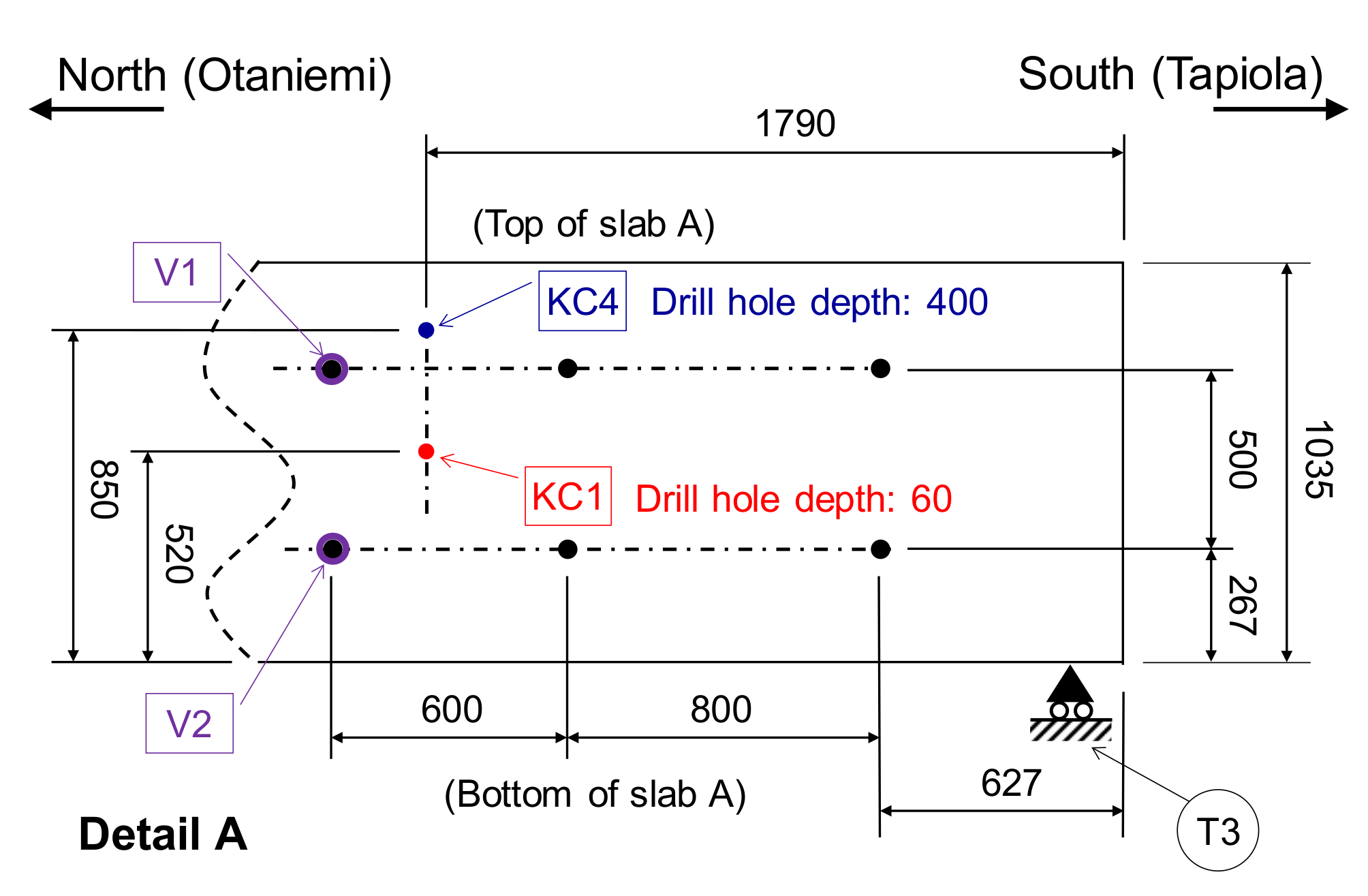
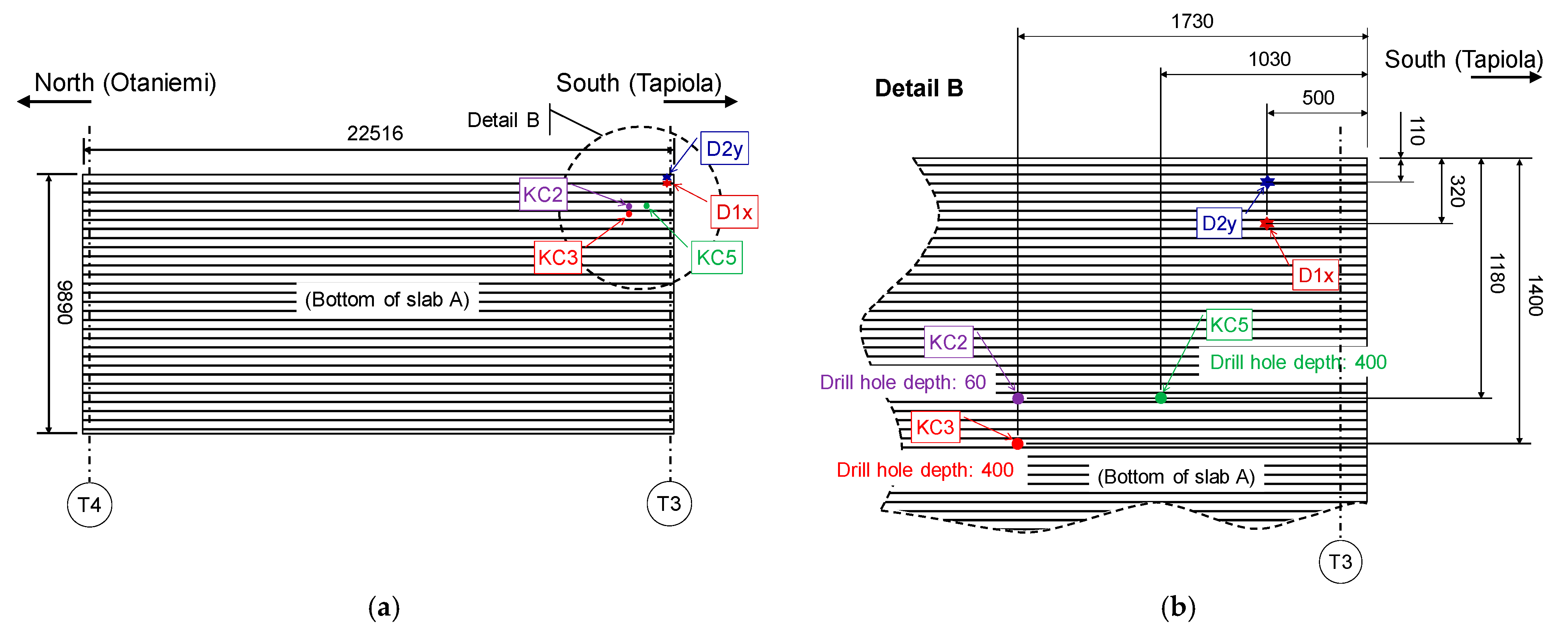
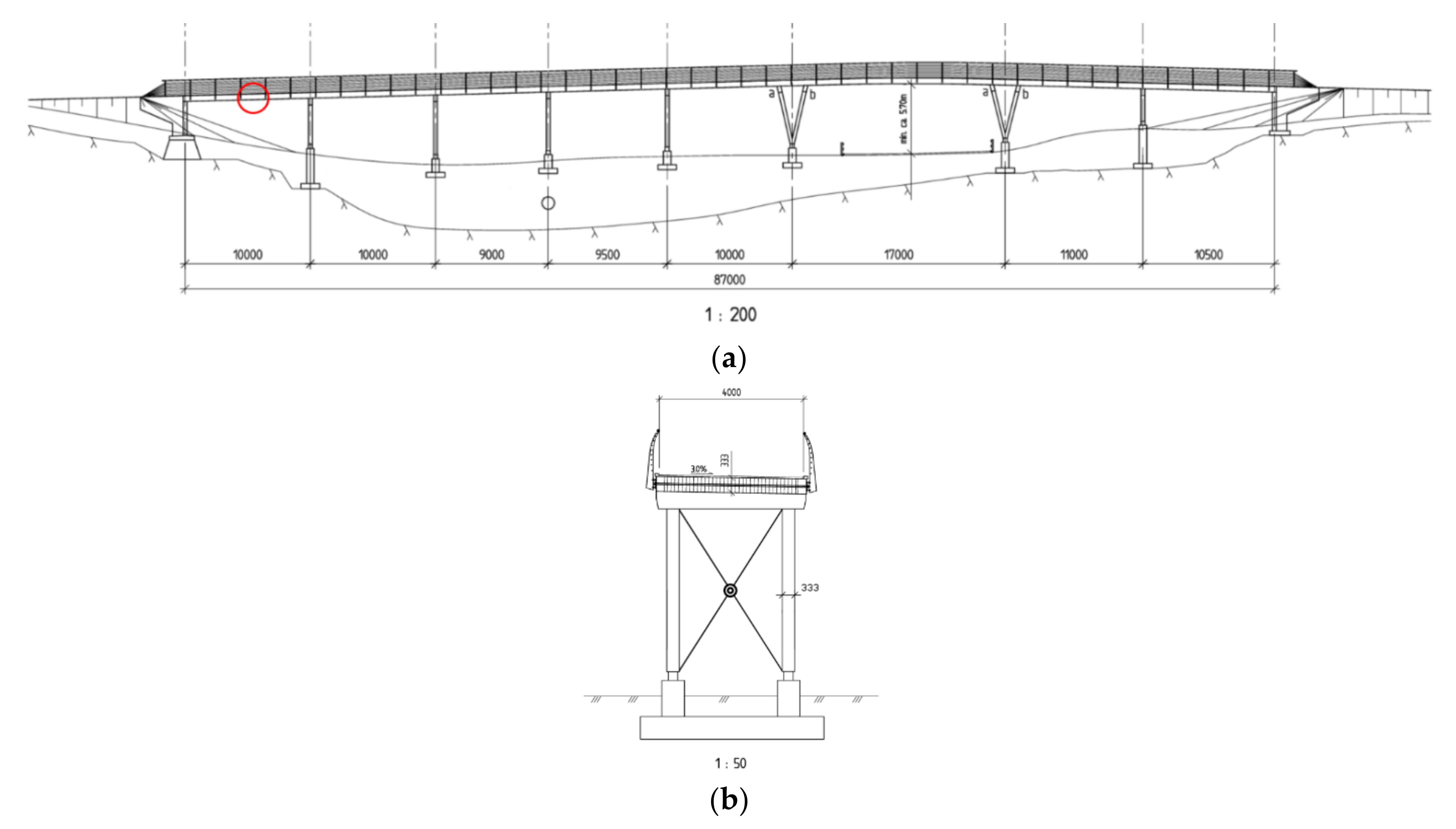
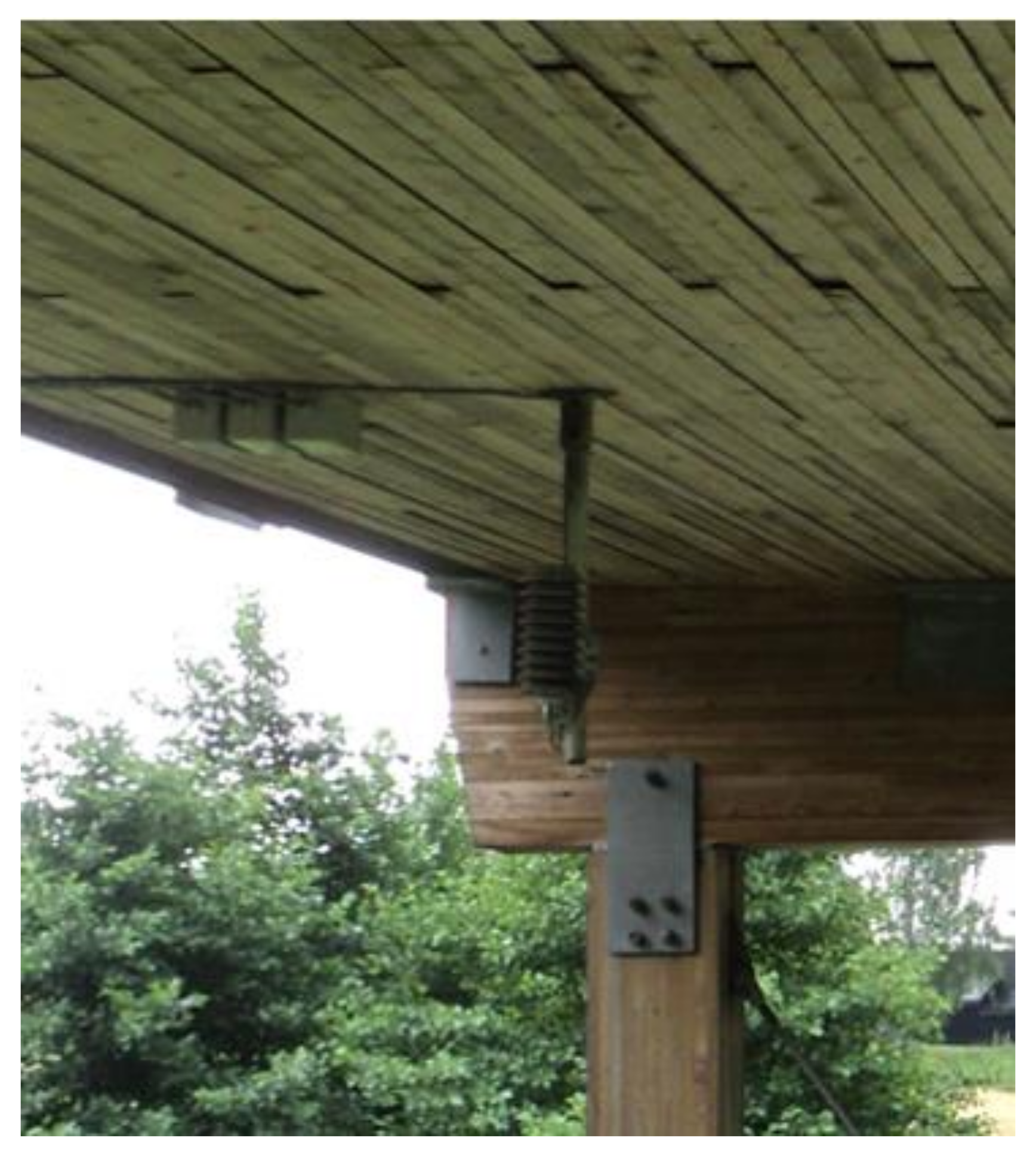
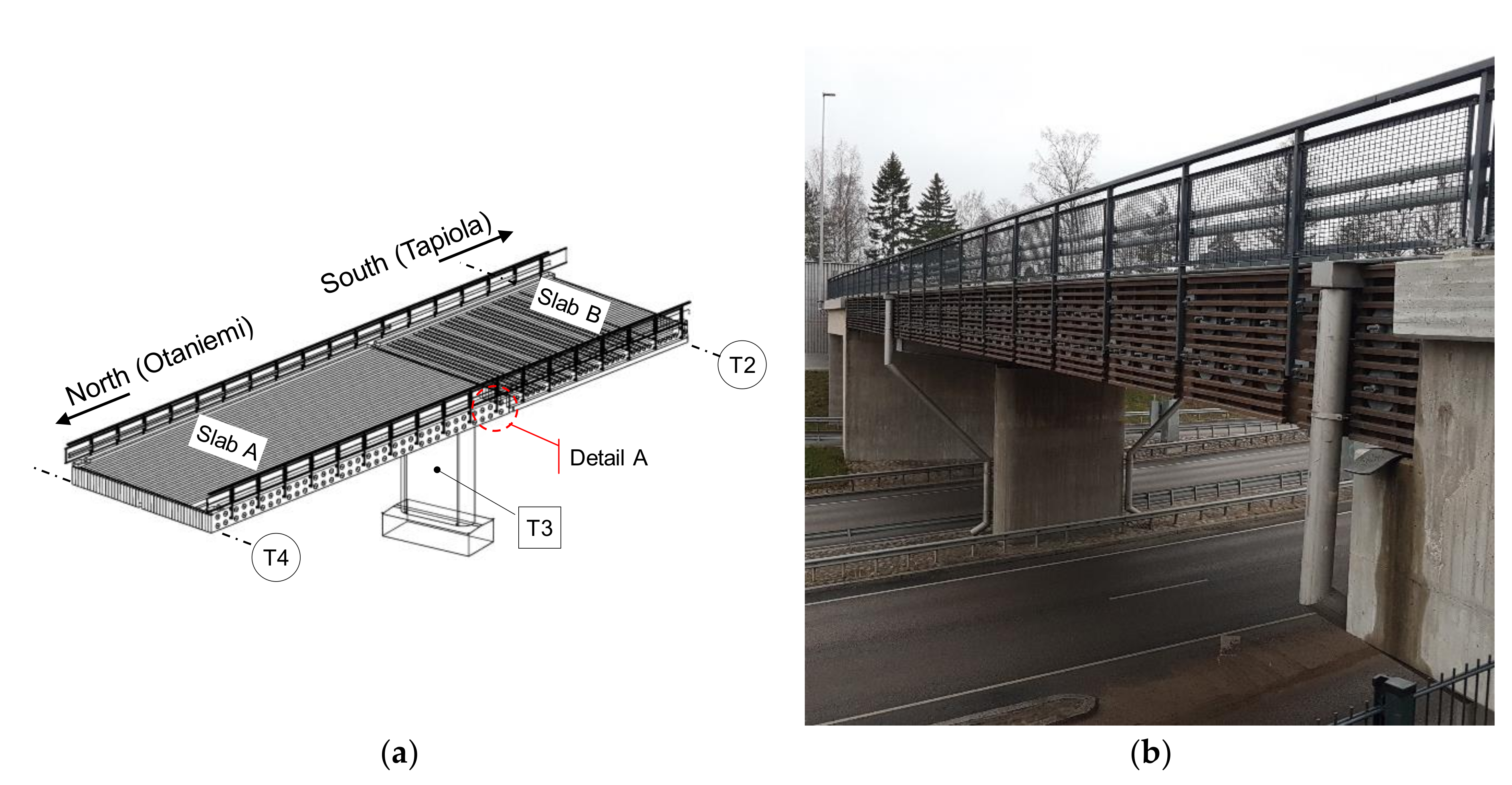
2.3. Case-Study: Sørliveien Bridge

Sørliveien Bridge (Figure 4 and Figure 5) is a pedestrian bridge built in summer 2005 in Akershus County, Norway, crossing a local road [24,25]. The owner was the Norwegian Public Road Administration. It is a slab bridge with eight spans and a total length of 87 m. The longest span is 17 m. The stress-laminated timber deck (48 × 333 mm) is composed of spruce glulam planks, which are untreated except for the edge planks of creosote-impregnated pine wood. The top layer consists of 60 mm asphalt with a moisture membrane of polymer modified bitumen (Topeka 4S) underneath. The bridge has been instrumented in August 2005 and monitored since then. The instrumentation is situated at the northern end and is logged every fourth hours.
The monitoring equipment (Figure 5) collects data about the loading of the high-strength steel bars, temperature and humidity of the wood at different depths from the surface, and temperature and humidity of the air from the weather station positioned on the bridge. The collected data is processed directly on the embedded computing unit and regularly transmitted to the central monitoring server over the internet.
Three load cells were installed to the prestressing bars loaded to 227 kN, on the northeast side of the bridge. The measurements from load cells are not discussed in this paper, because they are not directly needed for the hygro-thermal simulations. Temperature and relative humidity were measured by ten integrated humidity-temperature sensors Vaisala Humitter 50Y [27]. This type of sensor has an operating range from −40 °C to +60 °C and from 0 to 100% of the RH. Its length is 70 mm and the diameter 12 mm. Nine sensors were installed in three different depths from the bottom surface (20 mm, 166 mm and 308 mm) and three different planks, and one additional sensor was measuring the temperature and relative humidity of the ambient air.
The FEM model for the Sørliveien deck is a 3D slice of the lamella, with the width of 48 mm, height 333 mm and thickness 5 mm. The weather data in Figure 6 was the primary information needed for the hygro-thermal simulation, because the boundary conditions of the model are based on the external RH and T. The numerical analysis is carried out from August 2005 until the end of January 2010, since in this period the measurements are continuous. The initial relative humidity and temperatures are equal to those of the air (RH0 = 65%, T0 = 26 °C) and the initial moisture content in equilibrium with RH0 is MC0 = 13.3%.

2.4. Case-Study: Tapiola Bridge

The highway overpass in the Tapiola district of Espoo, Finland, was built in the Spring of 2019 and was recently opened to traffic (Figure 7). Two of its three spans are stress-laminated timber decks compressed by steel bars in the transverse direction. This short-/mid-span highway crossing serves local car and bus transportation. In the width direction, the bridge deck is composed of 46 timber beams. The widths of the beams are 0.215 m, and the heights equal to the deck thicknesses are 0.765 m for the 13.45 m span and 1.035 m for the 22.13 m span. The width of the decks is 9.89 m, which is near to its useful width 9.79 m. The basic dimensions of the bridge are listed in Table 1.
Five integrated humidity-temperature sensors, two displacement and two force sensors were installed on the bridge. The displacement sensors monitor vertical and horizontal motion, while the force sensors are measuring the tension force variation in the steel bars. In addition, the monitoring unit cabinet has two thermocouples for tracking its inside and outside temperature. The sensors are described in Table 2. Figure 8 shows the locations of the sensors. More details on the sensor locations are provided in Figure A1 and Figure A2 of Appendix B.
The sensors have wired connections to the monitoring unit. The unit itself is placed in the metal cabinet on the abutment of the bridge and it is connected to the electric grid and the internet. The devices and programmes of the unit are shown in Table 3.
Before the installation, the sensors were tested in the humidity-temperature controlled rooms at VTT Technical Research Centre of Finland Ltd (VTT). Only the temperature sensors (thermocouples), located inside and outside of the measurement enclosure were not calibrated, because they have lower precision requirements.
The force sensor calibration was performed with the test rig of VTT, and a calibration factor of 0.95 was found. The current measurement system is able to record the relative force shift/change of the pre-tension bars. Displacement sensors were not explicitly calibrated, instead the manufacturer’s instructions and precision requirements are followed [29].
The deck is protected with Valtti colour, an oil-based wood strain produced by Tikkurila [35]. According to the producer, this paint exhibits a low vapour resistance.
The FEM model for the deck is a 3D slice having a width of 107.5 mm (half of the lamination), height 1035 mm and thickness 5 mm. The numerical analysis of the Tapiola Bridge deck starts at the end of the construction time (April 2019) until October 2020, see the weather data in Figure 9, while the sensor-based monitoring started later (October 2019) and is on-going. The earlier starting of the numerical analysis demonstrates that the numerical models can assist the monitoring by predicting the hygro-thermal response of the SLTD also in the absence of measurements. The initial relative humidity and temperatures are equal to those of the air (RH0 = 65%, T0 = 0.85 °C) and the initial moisture content in equilibrium with RH0 is MC0 = 15.3%.

3. Results

3.1. Hygro-Thermal Response of the Deck of Sørliveien Bridge

The outputs of the finite element model are the temperature, the moisture content and the vapour pressure in the wood material.
Since the RH and T in wood were measured directly by the monitoring system, reference results for the validation of the numerical model were available from all of the nine integrated humidity-temperature sensors installed in the wood lamellas. For the purpose of investigation of MCs and moisture gradients near the surface of untreated wood exposed to the external climate, data measured at 20 mm from the bottom surface were selected for comparison with the numerical results.
Figure 10 shows the comparisons in terms of vapour pressures between the measured and numerical data. The directly measured RH in wood was multiplied by the saturated vapour pressure by using the same Equation (9) adopted for the numerical model. Figure 11 presents the comparison between measured and numerical values of temperatures. The results of the FEM calculation show a good correlation to the yearly variation of the monitored temperatures and measurement-based vapour pressures.
The numerical model assists the monitoring by allowing the evaluation of the MC from the bottom surface of the 3D slice until 20 mm, as shown in Figure 12. The numerical MCs close to the bottom surface are much higher than the ones at 20 mm from the surface that show small fluctuations (Figure 12a). The related moisture envelopes (minimum, maximum, average, 5th and 95th percentile), which show the trend of the moisture gradients, are presented in Figure 12b. A summary of the maximum and minimum MC values between the surface and 20 mm depth is shown in Table 4.

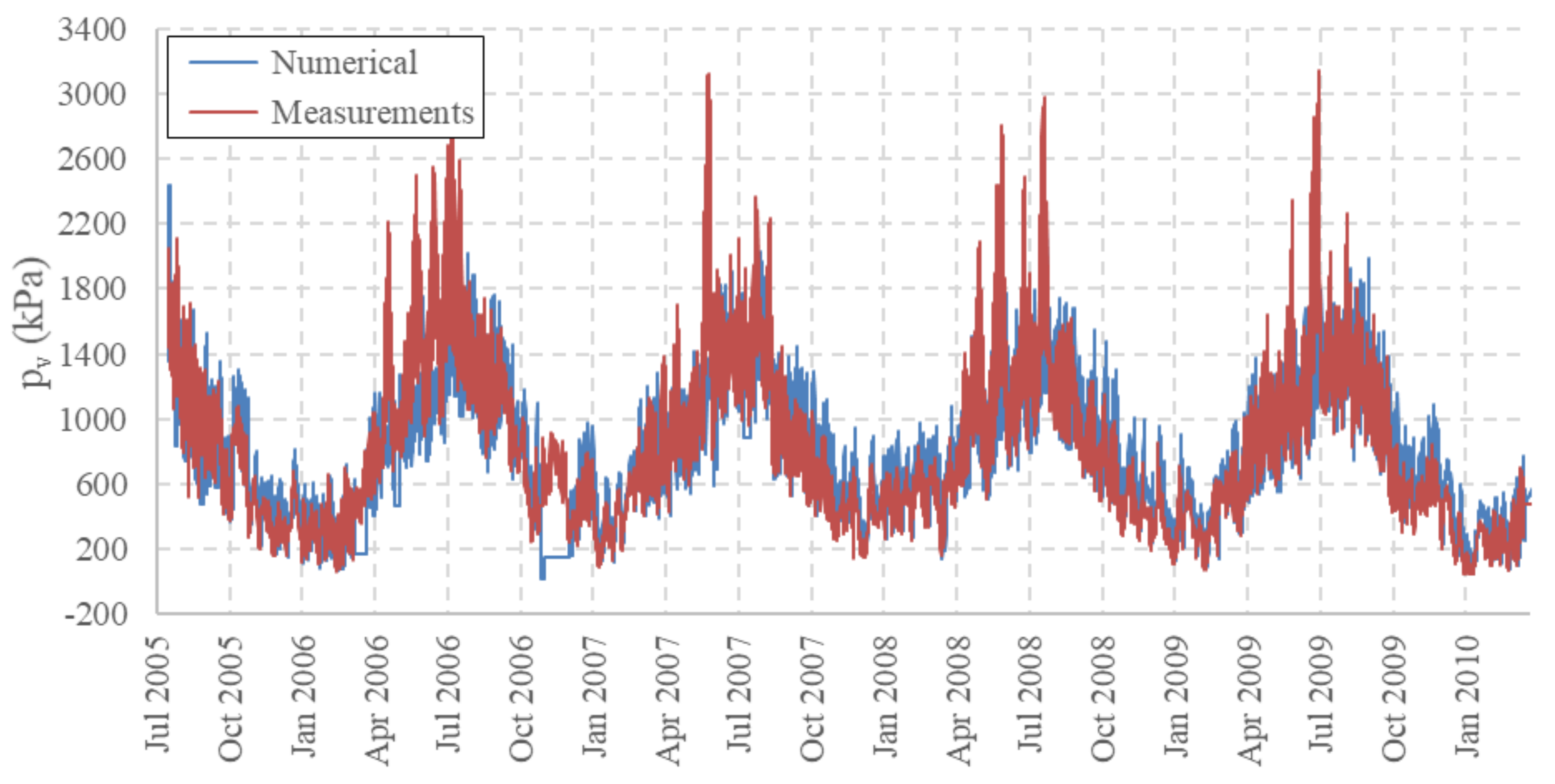
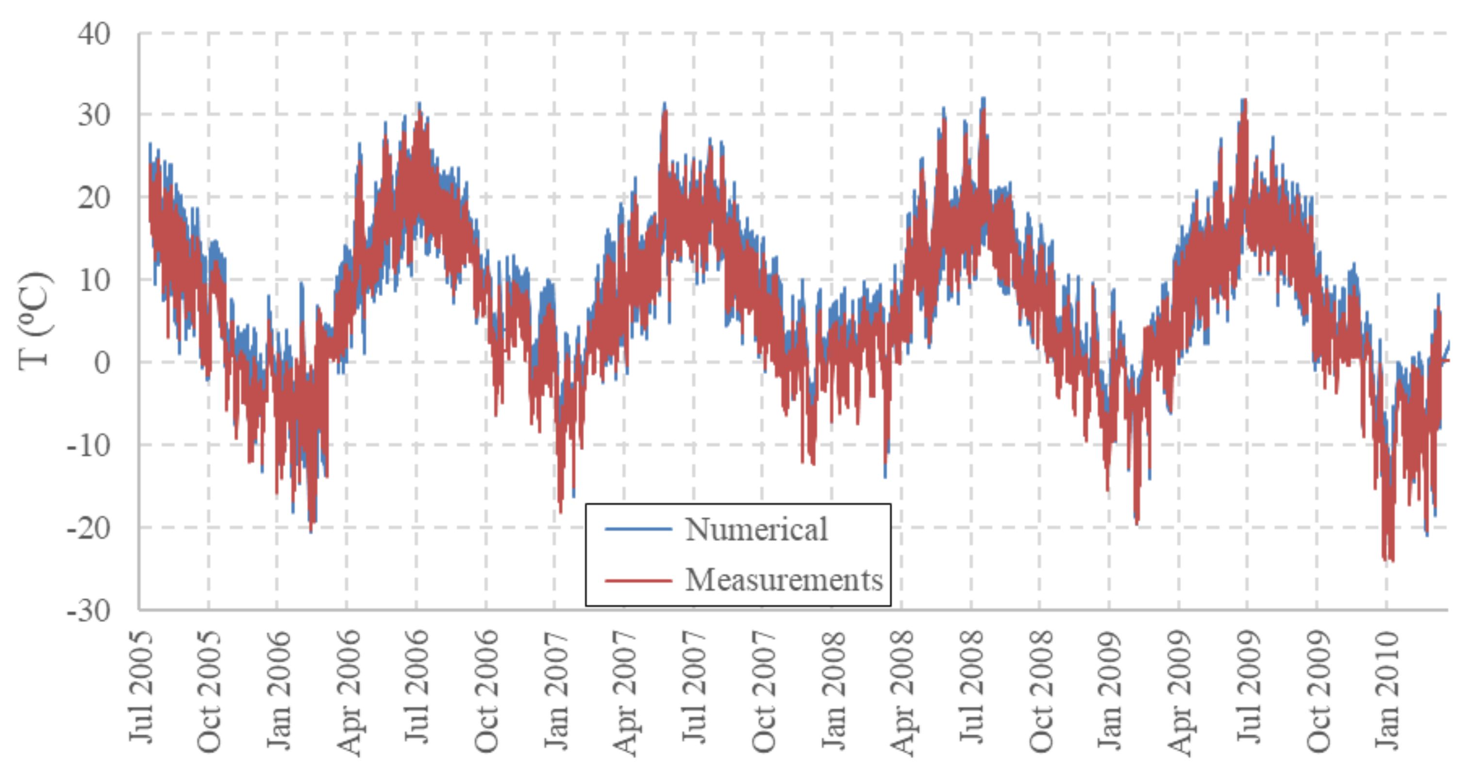
3.2. Hygro-Thermal Response of the Deck of Tapiola Bridge

In this case-study, in this case-study, the results of the FEM analysis are in good agreement with the yearly variation of the temperatures and vapour pressures monitored at 60 mm from the bottom surface in sensors KC1 and KC2 (Figure 13 and Figure 14). The larger temperatures measured in KC1 are because this sensor is located on the bridge side exposed to sun while KC2 is in the shadow. Since the model does not include the effect of solar radiation, the better comparison is with the data provided by sensor KC2 that is installed from the bottom of the deck.
The MC history at 60 mm from the bottom surface shows very small daily fluctuations while the numerical results closer to the surface are larger (Figure 15a). Figure 15b shows the minimum and maximum moisture envelopes during the monitoring time, as well as the 5th and 95th percentile from the external bottom surface to 60 mm depth. For this thick deck, a summary of the maximum and minimum MC values between the surface and 400 mm depth is shown in Table 5.

4. Discussion

The combination of the sensor-based monitoring and numerical model presented in the previous sections, allowed analysing the hygro-thermal response of the uncoated SLTD of Sørliveien Bridge in Norway and the thick painted SLTD of Tapiola Bridge in Finland. In addition to the temperature T and vapour pressure pv, the numerical model was able to provide quantitative values of the moisture content MC and the moisture gradients trends close to the surface that could be responsible of surface cracks, as shown in earlier works for large glulam beams of timber bridges [10,11,12] and in a research on the monitoring of large span timber structures [36]. In particular, we analysed the bottom part of decks which are sheltered from rain but subjected to both the continuously variable air humidity and temperature.
The uncoated deck of Sørliveien Bridge in Norway was analysed as a first case-study, and showed a relatively stable moisture behaviour after one year from the bridge erection. The main findings are listed below:
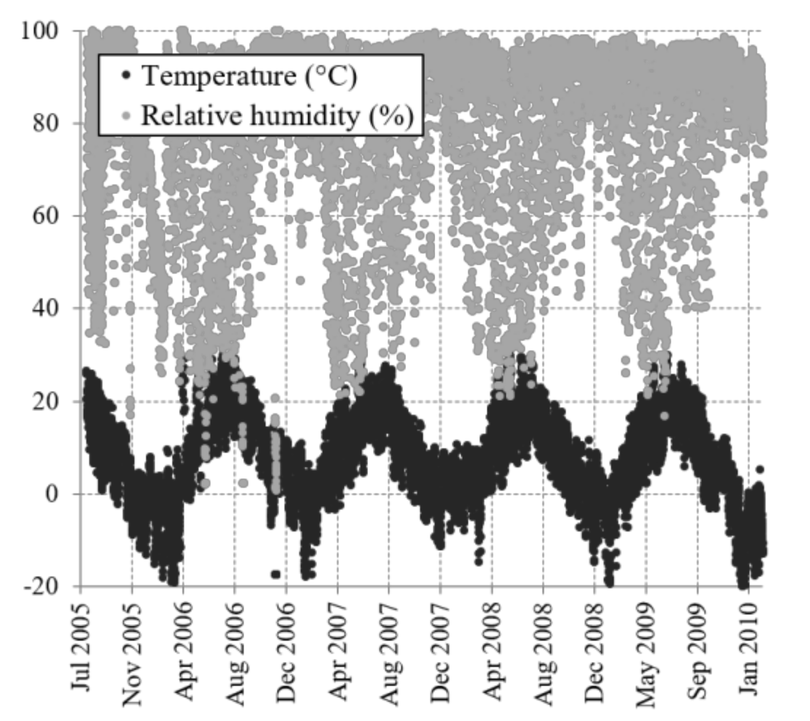
  • Referring to Table 4, the MC values on the bottom surface span in a range between 4% (reached at the beginning of summer 2006) and 25.8% (autumn 2005), are highest during the first year of the analysis and more stable during the successive years (Figure 12). The minimum and maximum MC values at 20 mm from the bottom surface are 12.5% at the beginning of the summer 2006, and 19% at the end of winter 2010. The results show that no significant changes of the average moisture content would be expected after the first year of the bridge service life, i.e., from June 2006 to January 2010.
  • High levels of MC over 20% were found only on the exposed surface at the bottom deck and in locations very close to this surface (Figure 12). These MC levels could be also critical for the wood durability [3], however the decay is a major problem mainly in the presence of liquid water due e.g., to rain and eventual water traps, and these cases were not investigated in the present work.
The painted and thick deck of Tapiola Bridge was analysed as second case-study, starting from an earlier stage after construction. The main findings are the following:
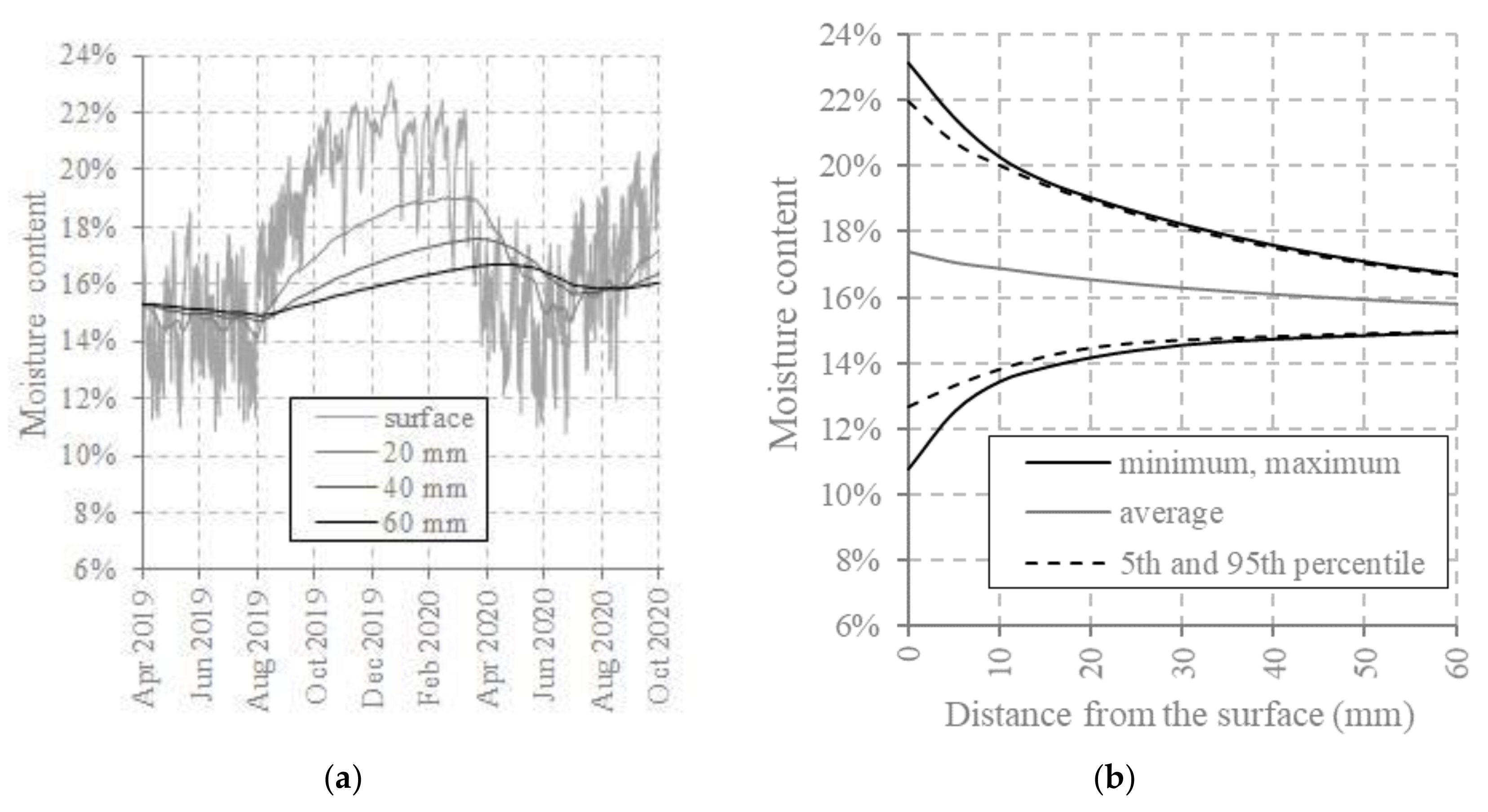
  • Referring to Table 5, the moisture contents on the bottom surface varies between 10.8%, reached at the beginning of the summer, and 23% at the beginning of the winter. In the internal locations, the maximum and minimum moisture contents are reached earlier depending on the maximum moisture penetration depth, which is about 200 mm (see Table 5). The maximum and minimum MC values in the location of the humidity-temperature sensor at 60 mm from the bottom surface are 16.7%, at the beginning of spring, and 14.9% at the end of summer.
  • High levels of MC (i.e., >20%) were found only on the exposed bottom surface and in locations very close to this surface. Compared to the MCs of Sørliveien Bridge, the peaks remained below 23% (Figure 15). This is because Tapiola Bridge is protected, even if the used paint has low vapour resistance (see Table A3 of Appendix A).
The following observations are based on the comparisons between the two case-studies:
  • Considering the MC results of Sørliveien Bridge, it could be estimated that also for Tapiola Bridge the average values of MC will not change significantly during the successive years.
  • The envelope curves shown in Figure 15b indicate similar levels of moisture gradients close to the surface as those of the Sørliveien Bridge’s deck (Figure 12b). The average MCs are around 16% up to 20 mm depth, and remain at an almost constant level up until 60 mm depth in Tapiola Bridge’s deck. Previous hygro-thermal models of SLTDs, based on single-phase moisture transport, found cupping deformations of around 16 mm and steel bar force losses of around 33% at these MC levels after 15 months [9].
The displacements and forces measured in the other sensors of the two monitoring systems can be simulated in future work by integrating the hygro-thermal analysis with a mechanical model for wood as in [9,12].
The embedded sensors and computational unit allow further expansion of the Internet of Things (IoT) network in order to efficiently exchange the monitoring data with passing vehicles and stationary objects of the road infrastructure. Moreover, combined with the results of the FEM simulation, the system can provide a comprehensive understanding of the bridge deck conditions in real time.

5. Conclusions

This paper proposed the use of an advanced multi-phase numerical model for wood below the fibre saturation point, previously introduced by some of the authors, to assist the monitoring of stress laminated timber decks by integrated humidity-temperature sensors.
The hygro-thermal simulation of a representative deck volume under Northern European climates supplements the sensor-based data. The simulation provides the distribution of the moisture content below the FSP, the temperature and the vapour pressure in the studied volume and allows to draw conclusions about the hygro-thermal response of the deck. However, the model does not include the effect of solar radiation and this is a task for future research. The modelling of the protective asphalt layer is also a topic for future work. The two analysed case-studies are sheltered from rain. To consider the effects of rain and possible water traps, the current model needs to be extended by introducing the variable concentration of free water in the lumens.
In future coupled hygro-thermo-mechanical models for SLTDs, the accurate evaluation of moisture contents is important for the prediction of moisture induced stresses which are responsible for surface cracking, cupping deformations and losses of the pre-stress force in steel bars.
The proposed method can be used to assist the monitoring techniques under Nordic climates contributing to maintenance cost reduction of timber bridge decks. FEM-assisted monitoring of bridges has a great potential to decrease the cost of instrumentation and increase safety. It can predict possible damages and communicate the results to other infrastructure components.

Author Contributions

Conceptualization, S.F., P.H., L.F.; methodology, S.F., P.H., H.B., K.K.; software, S.F., P.H., K.K.; validation, S.F., P.H., A.K.; formal analysis, S.F., P.H.; investigation, H.B., K.K.; resources, T.T.; data curation, P.H., K.K., H.B.; writing—original draft preparation, S.F., P.H.; writing—review and editing, P.H., L.F., T.T.; visualization, P.H., A.K.; supervision, S.F.; project administration, S.F.; funding acquisition, S.F., T.T. All authors have read and agreed to the published version of the manuscript.

Funding

This research was funded by WoodWisdom-Net project “Durable Timber Bridges” and by project “Delivering Fingertip Knowledge to Enable Service Life Performance Specification of Wood—Click Design”, which is supported under the umbrella of ERA-NET Cofund ForestValue by the Ministry of the Environment of Finland. ForestValue has received funding from the European Union’s Horizon 2020 research and innovation program. The Finnish Transport Infrastructure Agency (Väylävirasto) is a co-funder of the Click Design project.

Informed Consent Statement

Informed consent was obtained from all subjects involved in the study.

Data Availability Statement

The data presented in this study are available on request from the corresponding author. The data are not publicly available due to the agreements with the funding projects.

Acknowledgments

The authors wish to thank the Norwegian Public Road Administration for providing the monitoring data of Sørliveien Bridge. The Finnish Transport Infrastructure Agency (Väylävirasto) and the City of Espoo is acknowledged for supporting the monitoring of the Tapiola Bridge. The authors would like to warmly thank VTT colleagues Jukka Mäkinen, Mikko Kallio, Kalle Raunio, Pekka Halonen, Kari Korhonen for taking care of the on-going monitoring of Tapiola Bridge.

Conflicts of Interest

The authors declare no conflict of interest. Co-funder Väylävirasto (T.T.) participated in the interpretation of data, writing of the manuscript and in the decision to publish the results.

Appendix A

Table A1. Material parameters for the multi-Fickian model (all references can be found in [11]).
Water vapour diffusion tensor
D v = ξ v   2.31 · 10 5 p a t m p a t m +   p v T 273 1.81   m 2 s 1
  • Atmospheric pressure p a t m = 101325   Pa
  • Vapour pressure p v = c v R T / ( φ M H 2 O )
  • Gas constant R = 8.314   Jmol 1 K 1
  • Molecular mass of water M H 2 O = 18.02 × 10 3   kgmol 1
Components of reduction factor ξ v
ξ v L = 0.9 longitudinal
ξ v T = 0.12 transverse (*)
Bound water diffusion tensor
D b =   D 0 e x p E b R T   m 2 s 1
  • Activation energy of bound water diffusion
  • E b = 38.5 29 M C · 10 3   Jmol 1
Components of diagonal tensor D 0
D 0 L = 17.5 · 10 6   ( m 2 s 1 ) longitudinal
D 0 T = 7 · 10 6   m 2 s 1 transverse
Thermal conductivity tensor
K = ξ H G 0.2 + 0.38 M C + 0.024 Wm 1 K 1
  • Specific gravity of wood G = 0.693 G 0 / 0.653 + M C
  • G 0 = ϱ 0 / ϱ 0 w = dry wood density/water density
Components of reduction factor ξ H
ξ H L = 2.5 longitudinal
ξ H T = 1 transverse
Specific heat c w =   0.0011 T + M C 0.0323 1 + M C Jkg 1 K 1
Wood density ϱ = G 1 + M C ϱ w   kgm 3
Enthalpy of bound water
h b =   7.8955 · 10 5 4.476206 · 10 2 T + 2.274399 · 10 T 2 4.9553577 · 10 2   T 3 + 4.041035 · 10 5 T 4   Jkg 1
Enthalpy of water vapour
h v = 1.891879 × 10 6 + 2.56352 × 10 3 T 1.2360577 T 2   Jkg 1
Sorption reaction rate function
H c =   C 1 e x p C 2 c b c b l C 3   + C 4 c b < c b l C 1 e x p     C 2 2   c b c b l C 3   + C 4 c b > c b l
Constants
C 1 = 3.8 · 10 4 s 1
C 2 =   c 21 e x p c 22 R H +   c 23 e x p c 24 R H
C 3 = 80.0
C 4 = 5.94 · 10 7 s 1
c 21 = 3.579
c 22 = 2.21
c 23 = 1.591 · 10 3
c 24 = 14.98
Anderson–McCarthy model for sorption isotherms
M C b l , α = 1 f 2 α ln ln 1 R H f 1 α , α a , d
  • a and d refer to adsorption and desorption
  • f i α = j = 0 n b i j α T j ,     i 1 , 2
See Table A2
Permeances of the painted wood referred to wood temperature and air temperature:
k v w = 1 1 k w + 1 k p R T M H 2 O , k v a = 1 1 k w + 1 k p R T a M H 2 O
Thermal emission:
k T = 20 [W m−2 K−1]
See Table A3
(*) selected in this paper.
Table A2. Shape parameters for the temperature dependent adsorption and desorption functions.
αnb10α
[-]
b11α
[K−1]
b20α
[-]
b21α
[K−1]
a17.719−0.0115.0790.046
d19.739−0.017−13.4190.100
Table A3. Permeances of weak paint and uncoated wood.
PaintPermeance
[kg/m2 s Pa]
weak paint4.0 × 10−9
uncoated wood5.0 × 10−9

Appendix B

Figure A1. The locations of sensors in the side of the south-west corner of Slab A in the vicinity of the support T3 (see Figure 7a).
Applsci 11 00098 g0a1
Figure A2. Tapiola Bridge: (a) the prestressed glulam wooden Slab A of the bridge. (b) The locations of sensors in the bottom of Slab A in the vicinity of the slab’s south-west corner near the support T3 (see Figure 7a).
Applsci 11 00098 g0a2

References

  1. European Committee for Standardization. EN 1990: Eurocode: Basis of Structural Design; European Committee for Standardization: Brussels, Belgium, 2002. [Google Scholar]
  2. Obataya, E. Characteristics of aged wood and Japanese traditional coating technology for wood protection. In Proceedings of the Actes de la Journée D’étude Conserver Aujourd’hui: Les “Vieillissements” du Bois, Cité de la Musique, Paris, France, 2 February 2007. [Google Scholar]
  3. Brischke, C.; Meyer-Veltrup, L. Modelling timber decay caused by brown rot fungi. Mater. Struct. 2016, 49, 3281–3291. [Google Scholar] [CrossRef]
  4. Wacker, J. Cold Temperature Effect on Stress-Laminated Timber Bridges: A Laboratory Study; Research Paper FPL–RP–605; U.S. Department of Agriculture, Forest Service, Forest Products Laboratory: Madison, WI, USA, 2003.
  5. Scharmacher, F.; Müller, A.; Brunner, M. Asphalt surfacing on timber bridges. In Proceedings of the COST-Timber Bridges, Biel, Switzerland, 25–26 September 2014; Franke, S., Franke, B., Widmann, R., Eds.; Bern University of Applied Sciences: Bern, Switzerland, 2014. [Google Scholar]
  6. Aasheim, E. Nordic timber bridge program—An overview. In Proceedings of the International Wood Engineering Conference, New Orleans, LA, USA, 21–28 October 1996; Gopu, V.K.A., Ed.; International Wood Engineering Conference: New Orleans, LA, USA, 1996. [Google Scholar]
  7. Horn, H. Rapport Oppdrag Nr. 310332: Monitoring Five Timber Bridges in Norway—Results 2012; Norsk Treteknisk Institut: Oslo, Norway, 2013. [Google Scholar]
  8. Ministry of the Environment, Department of the Built Environment. Wood Building Programme. Available online: https://ym.fi/en/wood-building (accessed on 14 November 2020).
  9. Pousette, A.; Malo, K.; Thelandersson, S.; Fortino, S.; Salokangas, L.; Wacker, J. Durable Timber Bridges—Final Report and Guidelines; SP Report 25; Research Institutes of Sweden RISE: Skellefteå, Sweden, 2017. [Google Scholar]
  10. Fortino, S.; Genoese, A.; Genoese, A.; Nunes, L.; Palma, P. Numerical modelling of the hygro-thermal response of timber bridges during their service life: A monitoring case-study. Constr. Build. Mater. 2013, 47, 1225–1234. [Google Scholar] [CrossRef]
  11. Fortino, S.; Hradil, P.; Genoese, A.; Genoese, A.; Pousette, A. Numerical hygro-thermal analysis of coated wooden bridge members exposed to Northern European climates. Constr. Build. Mater. 2019, 208, 492–505. [Google Scholar] [CrossRef]
  12. Fortino, S.; Hradil, P.; Metelli, G. Moisture-induced stresses in large glulam beams. Case study: Vihantasalmi Bridge. Wood Mater. Sci. Eng. 2019, 14, 366–380. [Google Scholar] [CrossRef]
  13. Fragiacomo, M.; Fortino, S.; Tononi, D.; Usardi, I.; Toratti, T. Moisture-induced stresses perpendicular to grain in cross-sections of timber members exposed to different climates. Eng. Struct. 2011, 33, 3071–3078. [Google Scholar] [CrossRef]
  14. Niklewski, J.; Fredriksson, M. The effects of joints on the moisture behaviour of rain exposed wood: A numerical study with experimental validation. Wood Mater. Sci. Eng. 2019, 1–11. [Google Scholar] [CrossRef] [Green Version]
  15. Florisson, S.; Vessby, J.; Mmari, W.; Ormarsson, S. Three-dimensional orthotropic nonlinear transient moisture simulation for wood: Analysis on the effect of scanning curves and nonlinearity. Wood Sci. Technol. 2020, 54, 1197–1222. [Google Scholar] [CrossRef]
  16. Krabbenhøft, K. Moisture Transport in Wood: A Study of Physical-Mathematical Models and their Numerical Implementation. Ph.D. Thesis, Technical University of Denmark, Lyngby, Denmark, 2004. [Google Scholar]
  17. Frandsen, H.L. Selected Constitutive models for simulating the hygromechanical response of wood. Ph.D. Thesis, Department of Civil Engineering Aalborg University, Aalborg, Denmark, 2007. [Google Scholar]
  18. Eitelberger, J.; Hofstetter, K.; Dvinskikh, S.V. A multi-scale approach for simulation of transient moisture transport processes in wood below the fiber saturation point. Compos. Sci. Technol. 2011, 71, 1727–1738. [Google Scholar] [CrossRef]
  19. Konopka, D.; Kaliske, M. Transient multi-Fickian hygro-mechanical analysis of wood. Comput. Struct. 2018, 197, 12–27. [Google Scholar] [CrossRef]
  20. Huc, S.; Svensson, S.; Hozjan, T. Hygro-mechanical analysis of wood subjected to constant mechanical load and varying relative humidity. Holzforschung 2018, 72, 863–870. [Google Scholar] [CrossRef]
  21. Autengruber, M.; Lukacevic, M.; Füssl, J. Finite-element-based moisture transport model for wood including free water above the fiber saturation point. Int. J. Heat Mass Transf. 2020, 161, 120228:1–120228:21. [Google Scholar] [CrossRef]
  22. Svensson, S.; Turk, G.; Hozjan, T. Predicting moisture state of timber members in a continuously varying climate. Eng. Struct. 2011, 33, 3064–3070. [Google Scholar] [CrossRef]
  23. Thalla, O.; Stiros, S.C. Wind-Induced Fatigue and Asymmetric Damage in a Timber Bridge. Sensors 2018, 18, 3867. [Google Scholar] [CrossRef] [PubMed] [Green Version]
  24. Kepp, H.; Dyken, T. Thermal cction on timber bridges temperature variation measured in the deck of 3 timber bridges in Norway. In Proceedings of the International Conference Timber Bridges (ICTB2010), Lillehammer, Norway, 12–15 September 2010; Malo, K.A., Kleppe, O., Dyken, T., Eds.; Tapir Academic Press: Trondheim, Norway, 2010. [Google Scholar]
  25. Dyken, T.; Kepp, H. Monitoring the moisture content of timber bridges. In Proceedings of the International Conference Timber Bridges (ICTB2010), Lillehammer, Norway, 12–15 September 2010; Malo, K.A., Kleppe, O., Dyken, T., Eds.; Tapir Academic Press: Trondheim, Norway, 2010. [Google Scholar]
  26. Frandsen, H.L. Modelling of Moisture Transport in Wood: State of the Art and Analytic Discussion, 2nd ed.; Aalborg University: Aalborg, Denmark, 2005. [Google Scholar]
  27. Vaisala Oyj Home Page. Available online: https://www.vaisala.com/ (accessed on 24 November 2020).
  28. Hottinger Brüel & Kjaer GmbH Home Page. Available online: https://www.hbm.com/ (accessed on 24 November 2020).
  29. Opkon Optik Elektronik Kontrol San. Tic. Ltd. Şti Home Page. Available online: https://www.opkon.com.tr/ (accessed on 24 November 2020).
  30. Koski, K. Instrumentation of Tapiolantien Risteyssilta (Bridge); Research Report VTT-R-00837-19; Technical Research Centre of Finland: Espoo, Finland, 2019. [Google Scholar]
  31. Advantech, Co., Ltd. Home Page. Available online: https://www.advantech.com/ (accessed on 24 November 2020).
  32. National Instruments. Home Page. Available online: http://www.ni.com/ (accessed on 24 November 2020).
  33. DWS remote Control. Home Page. Available online: https://www.dwservice.net/ (accessed on 24 November 2020).
  34. Phoenix Contact. Home Page. Available online: https://www.phoenixcontact.com/ (accessed on 24 November 2020).
  35. Tikkurila Valtti Color Safety Data Sheet. Available online: https://tikkurila.com/sites/default/files/valtti-color-sds-en.pdf (accessed on 14 November 2020).
  36. Dietsch, P.; Gamper, A.; Merk, M.; Winter, S. Monitoring building climate and timber moisture gradient in large-span timber structures. J. Civil. Struct. Health Monit. 2015, 5, 153–165. [Google Scholar] [CrossRef]
Figure 1. Sørliveien Bridge. (a) Side view of the whole bridge structure. (b) Detail of the stress-laminated timber (SLT) deck protecting the bridge.
Applsci 11 00098 g001
Figure 2. Scheme of the water phases and sorption phenomena in wood. (a) Below the fibre saturation point (FSP): bound water in the wood cell walls, water vapour in the lumens and sorption rate between bound water and water vapour phases ( c ˙ b v ). (b) Above the FSP: Bound water in the wood cell walls, water vapour and free water in the lumens, sorption rates between bound water and water vapour ( c ˙ b v ) and between water vapour and bound water ( c ˙ w b ), and evaporation/condensation rate between free water and water vapour ( c ˙ w v ).
Applsci 11 00098 g002
Figure 3. Scheme of a 3D vertical slice of the timber deck for the hygro-thermal analysis. The asphalt layer is not modelled.
Applsci 11 00098 g003
Figure 4. Sørliveien Bridge in Norway. (a) Side view with location of sensors (red circle). (b) Cross section showing the SLT deck with 333 mm thickness.
Applsci 11 00098 g004
Figure 5. Sørliveien Bridge. Detail of the bottom deck with the monitoring equipment.
Applsci 11 00098 g005
Figure 6. Sørliveien Bridge. Weather data measured between 2005 and 2010.
Applsci 11 00098 g006
Figure 7. Tapiola Bridge. (a) The scheme of the transverse prestressed glulam wooden slabs of the bridge where T2, T3 and T4 indicate the support, reproduced from [30] with permission from VTT publications. Detail A is shown in Appendix B. (b) A picture with the view of the bridge.
Applsci 11 00098 g007
Figure 8. Tapiola Bridge. Photos of the sensor locations: (a) from the bottom; (b): from the lateral side. See the details about the locations of all sensors in Appendix B.
Applsci 11 00098 g008
Figure 9. Tapiola Bridge. Weather data measured between 2019 and 2020.
Applsci 11 00098 g009
Figure 10. Sørliveien Bridge. Comparison between measurement-based and numerical vapour pressures in wood at 20 mm from the bottom surface.
Applsci 11 00098 g010
Figure 11. Sørliveien Bridge. Comparison between measured and numerical temperatures in wood at 20 mm from the bottom surface.
Applsci 11 00098 g011
Figure 12. Sørliveien Bridge. Moisture content predicted by the finite element method (FEM) between the bottom surface and 20 mm depth. (a) MC vs. time. (b) Moisture envelopes (minimum, maximum, average, 5th and 95th percentile) from the external surface to 20 mm.
Applsci 11 00098 g012
Figure 13. Tapiola Bridge. Comparison between numerical temperatures in wood and measurements in sensors KC1 and KC2 at 60 mm from the surface.
Applsci 11 00098 g013
Figure 14. Tapiola Bridge. Comparison between numerical vapour pressures in wood and measurements in sensor KC2 at 60 mm from the bottom surface. In red the vapour pressure measurements in sensor KC1 at 60 mm from the lateral side exposed to the afternoon sun.
Applsci 11 00098 g014
Figure 15. Tapiola Bridge. (a) Moisture contents from the external surface of the deck until 60 mm depth. (b) Moisture envelopes (minimum, maximum, average, 5th and 95th percentile) from the external surface to 60 mm.
Applsci 11 00098 g015
Table 1. Tapiola Bridge decks.
Span13.45 m22.13 m11.8 m
Materialstress-laminated timberstress-laminated timberconcrete
Timber deck thickness0.765 m1.035 mn/a
Useful deck width9.79 m9.79 m13.13 m
Table 2. The installed sensors in Tapiola Bridge deck.
No.IDSensor TypeModel
1KC1Humidity and temperatureHMP110 [27]
2KC2Humidity and temperatureHMP110
3KC3Humidity and temperatureHMP110
4KC4Humidity and temperatureHMP110
5KC5Humidity and temperatureHMP110
6V1ForceC6A [28]
7V2ForceC6A
8D1xSlab longitudinal displacementELPC100 linear potentiometer of OPKON [29]
9D2y Slab vertical displacementELPC 100 linear potentiometer of OPKON
Table 3. The devices and software of the monitoring unit.
Industrial PC:Advantech [31]
Measurement software:Labview [32]
Remote desktop software:DWAgent [33]
Data acquisition chassis:NI cDAQ-9174 [32]
Data acquisition devices:NI 9211 (thermocouple) [32]
NI 9205 (temperature, moisture) [32]
NI 9237 (Force) [33]
Power supply: Quint Power [34]
Enclosure internal thermostat
Enclosure heater
Thermocouples
Table 4. Sørliveien Bridge. Numerical moisture content (MC) peaks at the bottom surface and 6, 12, 20 mm from the surface.
Distance from Bottom (mm)Max MC (%)DateMin MC (%)Date
025.831 October 2005426 May 2006
623.212 November 20058.927 May 2006
1221.219 January 200811.128 May 2006
201926 February 201012.57 June 2006
Table 5. Tapiola Bridge. Numerical MC peaks at the bottom surface and 20, 60, 200 and 400 mm from the surface.
Distance from Bottom (mm)Max MC (%)DateMin MC (%)Date
023.125 December 201910.825 June 2020
201915 March 202014.18 August 2019
6016.719 April 202014.910 August 2019
20015.430 September 202015.318 December 2019
40015.312 April 201915.325 June 2020
Publisher’s Note: MDPI stays neutral with regard to jurisdictional claims in published maps and institutional affiliations.

