Adaptive Semi-Active Suspension and Cruise Control through LPV Technique

Abstract

Several studies exist on topics of semi-active suspension and vehicle cruise control systems in the literature, while many of them just consider actual road distortions and terrain characteristics, these systems are not adaptive and their subsystems designed separately. This study introduces a new method where the integration of look-ahead road data in the control of the adaptive semi-active suspension, where it is possible to the trade-off between comfort and stability orientation. This trade-off is designed by the decision layer, where the controller is modified based on prehistorical passive suspension simulations, vehicle velocity and road data, while the behavior of the controller can be modified by the use of a dedicated scheduling variable. The adaptive semi-active suspension control is designed by using Linear Parameter Varying (LPV) framework. In addition to this, it proposes designing the vehicle velocity for the cruise controller by considering energy efficiency and comfort together. TruckSim environment is used to validate the operation of the proposed integrated cruise and semi-active suspension control system.

1. Introduction

Vehicle suspension has been a trending research topic for a long time due to its important role in road damage, ride comfort, vehicle safety and stability and overall performances of the vehicle. Multiple types of suspension systems such as active, passive and semi-active suspension systems are currently being studied and developed. Vehicle suspension systems can be classified in the three main categories, active, passive and semi-active according to their operation mode. The passive suspension is commonly used but limited to improve tire deformation or driving comfort. Hence, developing new type suspension be considered necessary. Active and semi-active suspension improves vehicle safety, driving comfort through minimizing effect if the road distortions and disturbances.

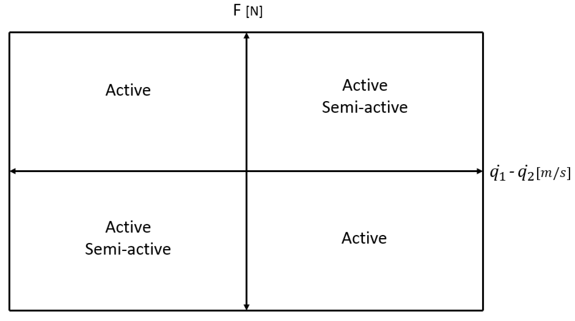
Active suspensions can store, dissipate or generate energy to the sprung and unsprung masses, although semi-active suspensions only dissipate the energy. Force-deflection speed space representation represents this difference, see Figure 1. A semi-active controller delivers forces within the two semi-active quadrants however, an active controller delivers force within the four quadrants.

The classic semi-active suspension control strategy is the skyhook damping control, which was first introduced by Reference [1]. This skyhook strategy has been widely used in the control for semi-active suspensions. This approaches aims to design an active suspension control so that the chassis is linked to the sky to reducing the vertical acceleration of the chassis and the axle independently of each other [2]. There are many studies, which have been considered the skyhook control strategy due to its simplicity to achieve comfort requirement [3,4,5,6]. While it improves ride comfort, it is limited to improve road-holding performance. The hybrid model predictive control (Hybrid MPC) method is currently widely used but it still lacks robustness properties and application is not easy [7]. ${\mathcal{H}}_{\infty }$ control approach has been carried out in many publications. This control strategy guarantees good performance in the road holding, vehicle stability and ride comfort [8,9], however, due to the fixed weighting of the performances, a dynamic control reconfiguration is not possible. Control reconfiguration is significant in terms of suspension control due to different road conditions and irregularities. Therefore, the semi-active suspension control in this study is founded on the Linear Parameter Varying (LPV) framework, which is available for the configuration by changing the scheduling variable [10,11,12]. According to the detailed literature review [13,14,15,16,17,18], they do not consider the integration of velocity design, oncoming road conditions and the trade-off between vehicle safety and driving comfort simultaneously.

This study introduces a new method where the integration of look-ahead road data in the control of the adaptive semi-active suspension. In addition to this, it proposes designing the vehicle velocity for the cruise controller by considering energy efficiency and comfort at the same time. TruckSim environment is used to validate the operation of the proposed integrated velocity and semi-active suspension control system. TruckSim environment has several sensors for the desired measurement signals and all results have been analyzed from data, which was provided by TruckSim simulation.

The paper is organized as follows—Section 2 involves energy-efficient cruise control. Section 3 presents the LPV controller synthesis and the control-oriented quarter-car model. Section 4 describes system integration and decision layer which is method of selection of scheduling variable $\rho$ depends on GPS based road data and look-ahead cruise control. Section 5 demonstrates the operation of the proposed method in high-fidelity TruckSim simulation environment with real road data. Finally, concluding remarks are presented in Section 6.

2. Energy Efficient Cruise Control

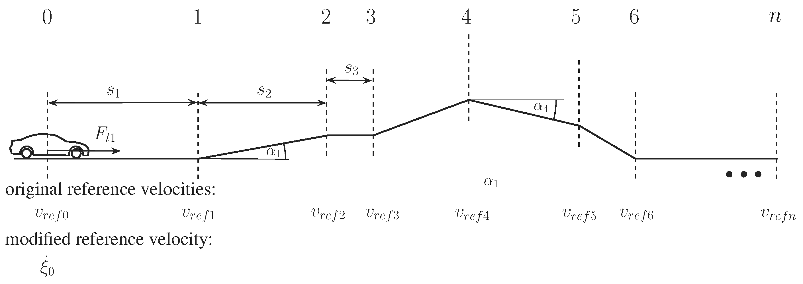
Reducing energy consumption by improving the driving style has drawn a lot of attention nowadays. Many assistance systems have been developed to derive energy-efficient driving styles and provide suggestions by human-machine interfaces. However, it is really hard for the driver to follow such suggestions perfectly. Thus, efficient cruise- control should be used for further vehicle technologies. The cruise control system automatically modifies a steady speed of a vehicle as set by the driver by setting the longitudinal control forces. Generally, adaptive cruise control systems are considered only the instantaneous effect of the road conditions, since they do not have information about onward road sections. But it is important to consider oncoming road sections The algorithm which performs look-ahead control has been already presented in a previous study [19]. As it is shown in Figure 2, the look-ahead distance L is divided into n number of road sections with $n+1$ number of points.

The rate of accelerations of the vehicle is considered between these points in order to make them constant. Thus, vehicle movement can be expressed as $s_1={\dot{\xi }}_0({\dot{\xi }}_1-{\dot{\xi }}_0)/\ddot{\xi }+({\dot{\xi }}_1-{{\dot{\xi }}_0)}^2/2\ddot{\xi }$, where ${\dot{\xi }}_0$ and ${\dot{\xi }}_1$ are the vehicle’s velocity at the initial point and at the first point respectively, $s_1$ is the distance between points and $\ddot{\xi }+(F_l-F_d)/m$ is the acceleration of the vehicle, where m is the mass of the vehicle, $F_l$ and $F_d$ are traction and disturbance force, respectively. Thus, the velocity of the first section point is calculated as following:

$${\dot{\xi }}_1^2={\dot{\xi }}_0^2+2{\dot{\xi }}_{s_1}+{\dot{\xi }}_0^2+\frac{2}{m}{s}_1(F_{l1}-F_{d1}),$$

(1)

where, ${\dot{\xi }}_1^2$ is velocity of the first section and defined as the reference velocity (${v^2}_{ref,1}$). This velocity relationship also applies for the next section as ${\dot{\xi }}_2^2={\dot{\xi }}_1^2+2{\dot{\xi }}_{s_2}$

Equation (2) is used to calculate the velocity of the vehicle for nth section point by using similar expression to Equation (1).

$${\dot{\xi }}_n^2={\dot{\xi }}_0^2+\frac{2}{m}\left(s_1{F}_{l1}-\sum _{i=1}^n{s}_i{F}_{di}\right)={v^2}_{ref,n},$$

(2)

where, $F_{di}$ is disturbance force and $F_{l1}$ is control force. Tracking the momentary value of the velocity also important and it can be considered in the following:

$${\dot{\xi }}_0^2\to {v^2}_{ref,0}.$$

(3)

Because of the collision risk, considering the preceding velocity on the lane is necessary:

$${\dot{\xi }}_0^2\to {v^2}_{lead}.$$

(4)

In the next step, weights($\gamma$) are applied to both road slope and reference velocity in Equation (2), while additional weights Q and W are applied in Equations (3) and (4), respectively. The all weights are sum up to one. The weight ${\gamma }_i$ expresses the rate of the road conditions, Q determines the tracking requirement of the reference velocity and W represents velocity tracking of the preceding vehicle, lead in order to avoid a collision. After consideration of the weights in the formulation, the following formula is written:

$${\dot{\xi }}_0^2+\frac{2}{m}{s}_1(1-Q-W)F_{l1}-\frac{2}{m}{s}_1(1-Q-W)F_{d1,o}=\vartheta ,$$

(5)

where

$$\vartheta =Q{v}_{ref,0}^2+\sum _{i=1}^n{\gamma }_i{v}_{ref,i}^2+\frac{2}{m}\sum _{i=1}^n(s_i{F}_{di,r}\sum _{j=i}^n{\gamma }_j).$$

(6)

It is assumed that speed limits and slope angles are known for each road section endpoints and optimal velocity is calculated by the following formula:

$$\lambda =\sqrt{\vartheta -2s_1(1-Q)({\ddot{\xi }}_0+g\sin \alpha )},$$

(7)

where $F_{di,r}=mgsin{\alpha }_i$ is the road disturbance force at each section point originated from the slopes on the look-ahead distance and $s_i$$i\in [1,n]$ is the road segment length with $L=\sum s_i$, $v_{ref,i}$ stands for the reference speed at every section endpoint. Q and ${\gamma }_i$ are used to scale the importance of the look-ahead and actual speed limits with following constraint: ${\gamma }_1+{\gamma }_2+\dots +{\gamma }_n+Q=1.$

There are two optimization problems which must be solved at the same time to meet the desired goals: both deviations from speed limits and longitudinal control force must be minimized. The first concentration is the energy efficiency which is fulfilled by the minimization of the longitudinal control force:

$$F_{l1}^2\to min.$$

The criterion the speed limit and road inclinations are considered by using appropriately chosen weights. The performance is met by the transformation of the quadratic form into the linear programming using the fmincon optimization algorithm. This is a nonlinear task, due to its weights. The optimization algorithm fmincon finds the minimum of a constrained nonlinear multivariable function. Therefore, a quadratic optimization problem is solved by Equation (8) with the following limitations:

$$0\le \overline{Q},{\overline{\gamma }}_i\le 1,\overline{Q}+\sum \overline{{\gamma }_i}=1$$

$${\overline{F}}_{l1}^2={({\beta }_0(\overline{Q})+{\beta }_1(\overline{Q}){\overline{\gamma }}_1+\dots +{\beta }_n(\overline{Q}){\overline{\gamma }}_n)}^2\to min.$$

(8)

In the next step, minimization in deviations from the speed limits is needed and it can be minimized by Equation (9).

$$|v_{ref,0}-{\dot{\xi }}_0[\to min.$$

(9)

Note that optimal solution for this latter criterion is to choose $\breve{Q}=1$ and ${\breve{\gamma }}_i=0$, $i\in [1,n]$.

The adequate balance between the conflicting performances is set by introducing two further performance weight $0\le R_1\le 1$ and $0\le R_2\le 1$, with the constraint $R_1+R_2=1$. Here, performance weight $R_1$ is related to the relationship of energy optimal operation of the look-ahead cruise controller, while $R_2$ is connected to the importance of minimizing the total travel time. These performance weights are applied as follows:

$$\begin{array}{cccc}Q\hfill & \hspace{1em}& \hspace{1em}& =R_1\overline{Q}+R_2\breve{Q}=1-R_1(1-\overline{Q})\end{array}$$

(10a)

$$\begin{array}{cc}\hfill {\gamma }_i& =R_1{\overline{\gamma }}_i+R_2{\breve{\gamma }}_i=R_1{\overline{\gamma }}_i,i\in \{1,\dots ,n\},\end{array}$$

(10b)

where $\overline{Q}$, ${\overline{\gamma }}_i$ are weights of the energy optimal solution and $\breve{Q}$ and ${\breve{\gamma }}_i$ are the weights of the time-optimal result.

3. Modeling and Control Synthesis of the Suspension System

A number of studies have already been developed related to the active and semi-active suspension system based on the quarter-car model with different methods. The methods such as ${\mathcal{H}}_{\infty }$ and linear-quadratic suspension control can provide guarantee good performance in both vehicle stability and passenger comfort but due to their fixed weighting of performance property, a dynamic control configuration is not possible. Hence, the Linear Parameter Varying (LPV) framework is a good solution for the dynamic control configuration to have road adaptation capabilities. Here, the semi-active suspension control is founded on the Linear Parameter Varying (LPV) framework, as already introduced in the previous studies [20,21].

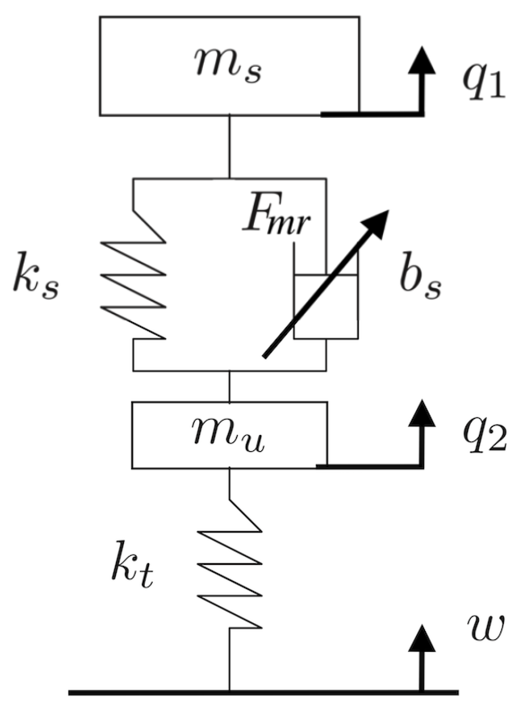
A model of the used two-degree-of-freedom quarter-car model that is more useful for researches is shown in Figure 3.

The dynamic model of the quarter-car semi-active suspension system and the actuator is written as follows:

$$\begin{array}{cc}\hfill m_s\ddot{q_1}+b_s(\dot{q_1}-\dot{q_2})+k_s(q_1-q_2)+F_{mr}& =0\hfill \end{array}$$

(11a)

$$\begin{array}{cc}\hfill m_u\ddot{q_2}+b_s(\dot{q_2}-\dot{q_1})+k_s(q_2-w)+k_s(q_2-q_1)-F_{mr}& =0,\hfill \end{array}$$

(11b)

where the actuator dynamics is approximated as

$${\dot{F}}_{mr}=-\frac{1}{\tau }{F}_{mr}+\frac{1}{\tau }u.$$

(12)

Here, $m_s$ and $m_u$ represent the quarter vehicle’s sprung mass and the unsprung mass, $k_t$ and $k_s$ state the stiffness of tire and spring, $b_s$ is the damping rate of the shock absorber, while $u=F$ is the control input of the system and $F_{mr}$ is the control force generated by the actuator. Note, that $q_1$ and $q_2$ are the vertical displacement of the sprung mass and the unsprung mass, while w expresses road disturbance.

The state vector x is selected as $x={\left[\begin{array}{ccccc}{x}_1& x_2& x_3& x_4& x_5\end{array}\right]}^T$, in which the components are shown in Equation (13).

$$\begin{array}{c}\hfill x_1=q_1\\ \hfill x_2=q_2\\ \hfill x_3=\dot{q_1}\\ \hfill x_4=\dot{q_2}\\ \hfill x_5=F_{mr},\end{array}$$

(13)

where $q_1$ and $q_2$ are vertical displacement of sprung and unsprung masses, $\dot{q_1}$ and $\dot{q_2}$ are vertical velocity of sprung and unsprung masses.

Thereafter, the system is given with Equation (11) is transformed into state-space representation form as follows:

$$\begin{array}{cc}\hfill \dot{x}& =Ax+B_{1}w+B_{2}u\hfill \end{array}$$

(14a)

$$\begin{array}{cc}\hfill z& =C_{1}x+D_{11}w+D_{12}u\hfill \end{array}$$

(14b)

$$\begin{array}{cc}\hfill y& =C_{2}x+D_{21}w+D_{22}u.\hfill \end{array}$$

(14c)

The main idea in order to find matrices is arranging the Equation (11) according to state vector components, performance vector components and the measured signal. Then, results are arranged according to Equation (14). and coefficient of the $x,w,u$ are clarified. These the coefficients($A,B_1,B_2,C_1,C_2,D_{11},D_{12},D_{21},D_{22}$) give us the matrices for the control design. These matrices are found below:

A = $\left[\begin{array}{ccccc}0& 0& 1& 0& 0\\ 0& 0& 0& 1& 0\\ -\frac{k_s}{m_s}& \frac{k_s}{m_s}& -\frac{b_s}{m_s}& \frac{b_s}{m_s}& -\frac{1}{m_s}\\ \frac{k_s}{m_u}& -\frac{k_s}{m_u}-\frac{k_t}{m_u}& \frac{b_s}{m_u}& -\frac{b_s}{m_u}& \frac{1}{m_u}\\ 0& 0& 0& 0& -\frac{1}{\tau }\end{array}\right]$

B1 = ${\left[\begin{array}{ccccc}0& 0& 0& \frac{k_t}{m_u}& 0\end{array}\right]}^T$, B2 = ${\left[\begin{array}{ccccc}0& 0& 0& 0& \frac{1}{\tau }\end{array}\right]}^T$, B = $\left[\begin{array}{cc}B1& B2\end{array}\right]$

C1 = $\left[\begin{array}{ccccc}-\frac{k_s}{m_s}& \frac{k_s}{m_s}& -\frac{b_s}{m_s}& \frac{b_s}{m_s}& -\frac{1}{m_s}\\ 1& -1& 0& 0& 0\\ 0& 1& 0& 0& 0\\ 0& 0& 0& 0& 1\end{array}\right]$, C2 = $\left[\begin{array}{ccccc}1& -1& 0& 0& 0\end{array}\right]$, C = $\left[\begin{array}{c}C1\\ C2\end{array}\right]$

$D_{11}$ = ${\left[\begin{array}{cccc}0& 0& -1& 0\end{array}\right]}^T$, $D_{12}$ = ${\left[\begin{array}{cccc}0& 0& 0& 0\end{array}\right]}^T$, $D_{21}$ = $\left[\begin{array}{c}0\end{array}\right]$, $D_{22}$ = $\left[\begin{array}{c}1\times {10}^{-10}\end{array}\right]$, D = $\left[\begin{array}{cc}{D}_{11}& D_{12}\\ D_{21}& D_{22}\end{array}\right]$

Table 1. Parameters of the suspension.

Parameters (Symbols)	Front Suspension	Rear Suspension	Unit
sprung mass($m_s$)	214	336	kg
unsprung mass ($m_u$)	40	40	kg
suspension stiffness ($k_s$)	30	60	kN/m
tire stiffness ($k_t$)	220	220	kN/m
damping ($b_s$)	50	50	N/m/s
time constant ($\tau$)	0.01	0.01	s

shows the nominal parameters of the quarter-car model for the rear and front suspension.

In this study, the unmodelled dynamics $\Delta$ are also considered with $\left|\Delta ({\omega }_1)\right|=0.25$ at low frequencies and $\left|\Delta ({\omega }_2)\right|=1$ at high frequencies, and is assumed to be stable with the norm condition ${∥\Delta ∥}_{\infty }<1$.

It is necessary to define the performance specifications in order to achieve a desired trade-off between ride comfort and road holding, while also taking control force into consideration. The acceleration of sprung mass of the vehicle must be minimized for the sake of increasing passenger comfort with the following optimization criterion:

$$z_1=\ddot{q_1}\to 0.$$

Stability of the vehicle is guaranteed with the minimization of the suspension deflection:

$$z_2=(q_1-q_2)\to 0.$$

In order to decrease variations of side force to guarantee stability, the dynamic tire load must be minimized with the optimization criterion:

$$z_3=(q_2-w)\to 0.$$

To avoid actuator saturation, the control force must also be considered with the optimization criterion:

$$z_4=F\to 0.$$

These performances are inserted in a performance vector

$$z={\left[\begin{array}{cccc}{z}_1& z_2& z_3& z_4\end{array}\right]}^T.$$

The measured signal is the relative displacement between the masses, that is, $y=x_1-x_2$. The control input u is the vertical force generated by the MR damper, with the dynamics listed in (12).

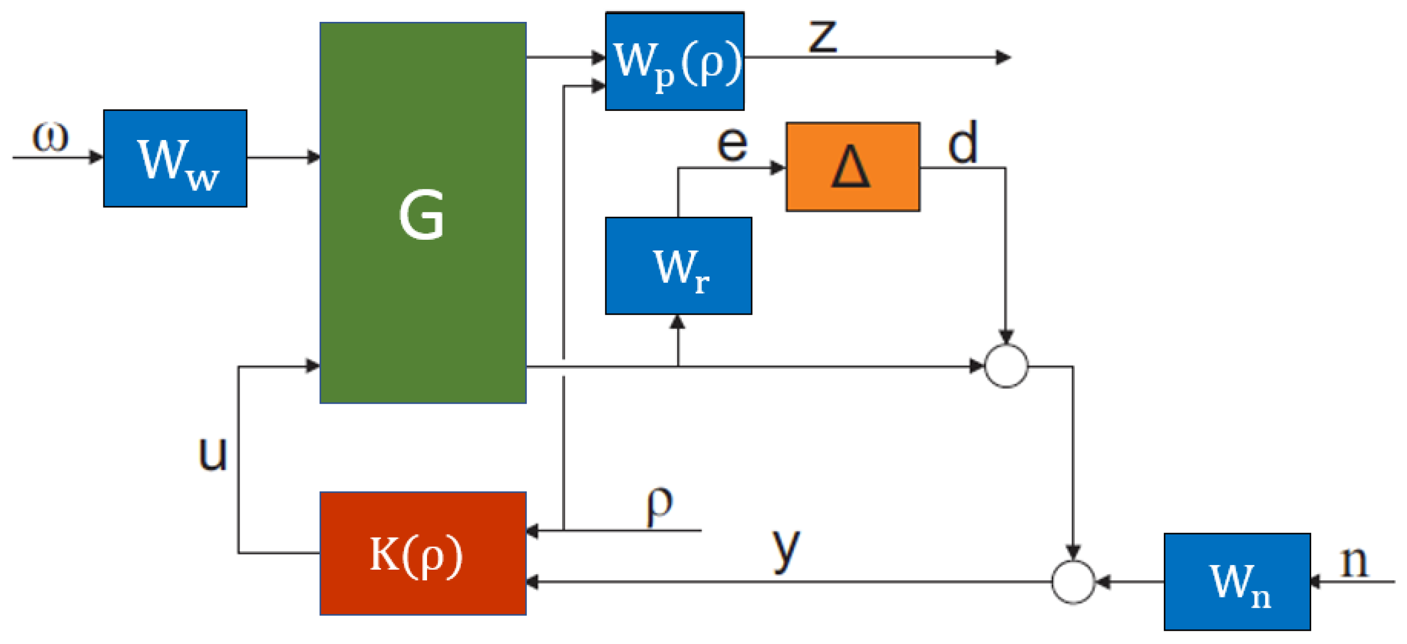
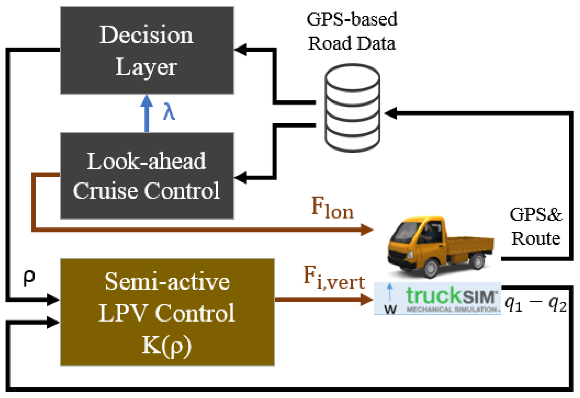
The presented high-level controller is founded on a weighting strategy formulated through a closed-loop architecture shown in Figure 4.

Here, G expresses the quarter-car control-oriented model defined in (14), K denotes the designed Linear Parameter Varying (LPV) controller characterized with the scheduling variable $\rho$ responsible for control reconfiguration, u is the control input, y is the measured output, n is the measurement noise, z represents the performance outputs and w is the road disturbance.

The uncertainties of the quarter-car model are considered with a weighting function of $W_r$ and $\Delta$. The weighting functions need to be considered as penalty functions, hence weights should be large where small signals are desired and vice versa. The goal of weighting function $W_n$ is to represent sensor noises with n measurement noise. The weighting function $W_w$ denotes the road disturbances with w road disturbance.

Weighting functions for performances $W_p$ is responsible to keep performances which are the sprung mass acceleration ($W_{p_a}$), suspension deflection ($W_{p_d}$), tire deformation ($W_{p_t}$) and control input ($W_{p_u}$) small over the required frequency range. $W_{p_a}$ represents passanger comfort, $W_{p_d}$ denotes directional stability and $W_{p_t}$ presents dynamic tire load.

Since the predefined performance designations may collide with each other, performance weighting functions $W_p$ need to be designed in a way that a relevant trade-off can be guaranteed between them. Additionally, to guarantee control reconfiguration in case one of the predefined performances becomes more important due to estimated future road conditions, a scheduling variable $\rho$$\in [0.01,0.99]$ is introduced to shape weighting function $W_{p_a}$, $W_{p_d}$ and $W_{p_t}$. Hence, these performance weighting functions related to passenger comfort and road holding are selected in a second-order proportional form as follows:

$$\begin{array}{cc}\hfill W_{p_a}& =\rho \frac{{\alpha }_{1}s+1}{T_{1}s+1}\hfill \end{array}$$

(15a)

$$\begin{array}{cc}\hfill W_{p_d}& =(1-\rho )\frac{{\alpha }_{2}s+1}{T_{2}s+1}\hfill \end{array}$$

(15b)

$$\begin{array}{cc}\hfill W_{p_t}& =(1-\rho )\frac{{\alpha }_{2}s+1}{T_{2}s+1},\hfill \end{array}$$

(15c)

where ${\alpha }_{1,2,3}$ and $T_{1,2,3}$ are designed parameters. Note, that weighting functions $W_{p_d}$, $W_{p_u}$, $W_r$, $W_n$ and $W_w$ are all given in similar linear and proportional form without containing the scheduling variable $\rho$.

The LPV performance problem is to choose a parameter-varying controller, which guarantees quadratic stability for the closed-loop system while the induced ${\mathcal{L}}_2$ norm from the disturbance $\omega$ to the performances z is smaller than the value $\gamma$, as described in Reference [22]. Therewith, the minimization task is given as:

$$\begin{array}{c}\hfill \underset{K}{inf}\underset{\varrho \in {\mathcal{F}}_{\mathcal{P}}}{sup}\underset{{∥w∥}_2\ne 0,w\in {\mathcal{L}}_2}{sup}\frac{{∥z∥}_2}{{∥w∥}_2}\le \gamma .\end{array}$$

(16)

The solution of an LPV problem is directed by the set of infinite-dimensional LMIs being satisfied for all $\rho \in {\mathcal{F}}_{\mathcal{P}}$, thus it is a convex problem. In practice, this problem is set up by gridding the parameter space and solving the set of LMIs that hold on the subset of ${\mathcal{F}}_{\mathcal{P}}$, see Reference [23]. The existence of a controller that solves the quadratic LPV $\gamma$-performance problem can be expressed as the feasibility of a set of the LMIs that can be solved numerically. The closed-loop LPV system is exponentially stable with its ${\mathcal{L}}_2-$gained less than $\gamma$, if there exists an $X(\rho )>0$ satisfying the following linear matrix inequality for all $\rho$, where $x^{T}X(\rho )x$ is a parameter-dependent Lyapunov function for the closed-loop system for all $\rho$ if a solution exists. The proof of the existence of the solution is available in study of Reference [24].

$$\left[\begin{array}{ccc}{A}_{cl}^{T}X+X{A}_{cl}^T+d/dt(X)& X{C}_{cl}& {\gamma }^{-1}{C}^T\\ B_{cl}^{T}X& -I& {\gamma }^{-1}{D}_{cl}^T\\ {\gamma }^{-1}{C}_{cl}& {\gamma }^{-1}{D}_{cl}& -I.\end{array}\right]$$

The result of the presented design is a reconfigurable LPV controller, $\rho =1$ stands where passenger comfort is preferred, whereas $\rho =0$ represents a controller considering stability and road holding of the vehicle, see Figure 5. When $\rho$ is between these edge values, a combination of performances is guaranteed by the controller.

Since the modeled MR damper has limitations on the control input force $u=F$, a semi-optimal solution is given as follows:

$$F=\left\{\begin{array}{c}{F}_{opt},\mathrm{if}\dot{q_1}(\dot{q_1}-\dot{q_2})>0\\ F_{pas},\mathrm{if}\dot{q_1}(\dot{q_1}-\dot{q_2})<0\end{array},\right.$$

(17)

where $F_{opt}$ is optimal force and $F_{pas}$ is passive suspension force.

4. System and Decision Integration Method

In this section, the system integration and decision layer with the method of selecting scheduling variable $\rho$ depending on GPS-based road data and look-ahead cruise control are described. The integration of the vertical and longitudinal control system is shown in Figure 6. There are various outputs that the controlled vehicle provides, however suspension deflection, GPS position, and prehistoric road data from these outputs are used in the integration of this system. GPS based road database consists of information about road conditions for each coordinate. According to GPS data, current oncoming road conditions can be known by using a GPS based road database. This information on road conditions is used for the decision layer and look-ahead cruise control. The look-ahead cruise control algorithm generates optimal velocity for the decision layer and longitudinal force($F_{lon}$) for the controlled vehicle, while a semi-active LPV controller generates damping force($F_{i,vert}$) for each wheel of the controlled vehicle by using suspension deflection measurement input and the value of the scheduling variable $\rho$.

Here, the decision logic layer is responsible for selecting $\rho$ based on road data, previous measurements and the calculated optimal velocity $\lambda$.

Multiple passive suspension simulations have been evaluated with different road types, velocities and $\rho$ values to analyze the performance results. The root mean square (RMS) value of these performances are calculated as below:

$$\begin{array}{c}\hfill {\mathcal{P}}^{va}=\sqrt{\frac{1}{T_a}{\int }_0^{T_a}{a}^2(t)dt}\\ \hfill {\mathcal{P}}^{td}=\sqrt{\frac{1}{T_t}{\int }_0^{T_t}{t_d}^2(t)dt},\end{array}$$

(18)

where $a(t)$ is the time-weighted acceleration, $t_d(t)$ is the time-weighted tire deformation, $T_a$ and $T_t$ is the number of acceleration and tire deformation values.

Table 2. Passive suspension simulation results.

Road Type	Velocity (km/h)	Vertical Acceleration(${\mathcal{P}}^{\mathbf{va}}$) $\left[{\mathit{\zeta }}^{\mathbf{va}}\right]$	Tire Deformation(${\mathcal{P}}^{\mathbf{td}}$) $\left[{\mathit{\zeta }}^{\mathbf{td}}\right]$
10cm bump	20	0.116 [8.7]	0.0006 [5.4]
	40	0.221 [16.6]	0.0013 [11.8]
	60	0.428 [32.3]	0.0024 [21.8]
	80	0.537 [40.5]	0.0039 [35.4]
Multiple bumps	20	0.370 [27.9]	0.0110 [100]
	40	0.431 [32.5]	0.0017 [15.4]
	60	0.466 [35.2]	0.0029 [26.3]
	80	0.444 [33.5]	0.0041 [37.2]
Sine-sweep	20	0.431 [32.5]	0.007 [63.6]
	40	0.751 [56.6]	0.002 [21.8]
	60	1.122 [84.6]	0.003 [27.2]
	80	1.326 [100]	0.011 [100]

shows the RMS values of vertical accelerations and tire deformations of passive suspension simulations for 10cm bump, multiple bumps, sine-sweep road types with different vehicle velocities. Note, that scaled vertical acceleration and tire deformation values are also calculated. These scaled performance values are calculated as follows:

$${\zeta }_{i,j}^k=\frac{{\mathcal{P}}_{i,j}^k}{{\mathcal{P}}_{max}^k},$$

(19)

where $\zeta$ is the scaled value, $\mathcal{P}$ states RMS value of the performance, k $\in [va,td]$, where $va$ is the vertical acceleration performance, $td$ is the tire deformation performance, i denotes the road type, j expresses the velocity of the vehicle.

It is assumed that the speed limit is 80 km/h for the vehicle, thus maximum velocity is 80 km/h in these passive suspension simulations.

The selection of the scheduling variable depends on the results of performances with the passive suspension system. The scaled performance value is compared to each velocity and road type. Equation (20) calculates the scheduling variable according to the relationship between performances as follows:

$$\rho =\left\{\begin{array}{cc}\frac{{\zeta }_{i,j}^{va}}{{\zeta }_{i,j}^{va}+{\zeta }_{i,j}^{td}}\hfill & \mathrm{if}{\zeta }_{i,j}^{va}>{\zeta }_{i,j}^{td}\hfill \\ 1-\frac{{\zeta }_{i,j}^{td}}{{\zeta }_{i,j}^{va}+{\zeta }_{i,j}^{td}}\hfill & \mathrm{if}{\zeta }_{i,j}^{td}>{\zeta }_{i,j}^{va}\hfill \\ 0.5\hfill & \mathrm{if}{\zeta }_{i,j}^{td}={\zeta }_{i,j}^{va}.\hfill \end{array}\right.$$

(20)

Here, the magnitude of the scaled values of vertical acceleration and tire deformation have significant importance to select the corresponding formula for the scheduling variable. As described in Section 3, the scheduling variable, $\rho =1$ stands where passenger comfort is preferred, whereas $\rho =0$ represents a controller considering stability and road holding of the vehicle. Thus, formulation of the scheduling variable is different for the case where ${\zeta }_{i,j}^{td}$ is greater than ${\zeta }_{i,j}^{va}$ and for the case where ${\zeta }_{i,j}^{va}$ is greater than ${\zeta }_{i,j}^{td}$. In the latter case scheduling variable is closer to ’1’, where controller works comfort-oriented. In the former case, scheduling variable is closer the ’0’, where controller works safety-oriented. For instance, let the road type be the sine-sweep irregularity and the vehicle velocity 60 km/h. Here, ${\zeta }_{sine-sweep,60}^{td}=27.2$ and ${\zeta }_{sine-sweep,60}^{va}=84.6$, thus ${\zeta }_{i,j}^{va}>{\zeta }_{i,j}^{td}$ case is fulfilled and first equation is used in (20). The calculated scheduling variable in this example is $\rho =0.75$, thus the behavior of the suspension is chosen to be more comfort oriented than stability oriented. The selected scheduling variables for the simulation are shown in

Table 3. Selected scheduling variable.

Road Type	Location (m)	Selected $\mathit{\rho }$
Multiple bumps	200	0.52
10 cm bump	950	0.6
10 cm bump	2000	0.54
Multiple bumps	2200	0.47
Sine-sweep	2650	0.5

, while a detailed description of irregularities and simulation route will be explained in Section 5.

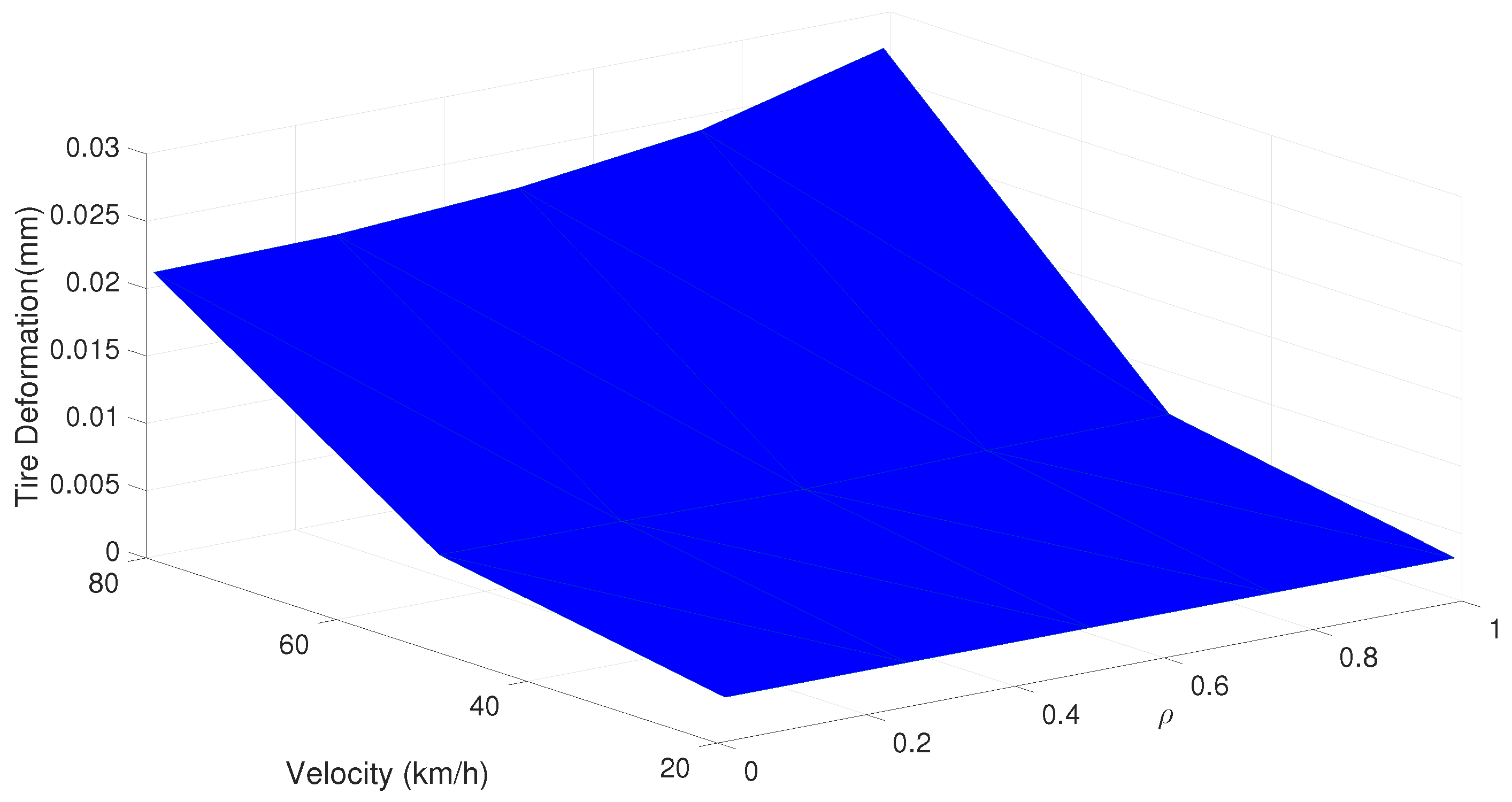
Note, that multiple simulations have been evaluated with the semi-active suspension to anaylze the scheduling variable-performance-velocity relationship, while one of these results are visualized in Figure 7. This figure shows the tire deformation surface map of a 10 cm bump road. It is well demonstrated that tire deformation is larger with higher velocities, while tire deformation decreases as $\rho$ approaches zero.

5. Simulation Results

A compact utility truck is selected for the simulation with independent rear and the front suspension and half a tonne of payload. Parameters of the simulated truck are shown in

Table 4. Vehicle parameters.

Parameter	Value	Unit
Truck mass ($m_t$)	760	kg
Payload mass ($m_p$)	500	kg
Distance from C.G to front axle ($l_1$)	0.55	m
Distance from C.G to rear axle ($l_2$)	1.375	m
Track width (b)	1.26	m
Height of COG ($h_{COG}$)	0.813	m
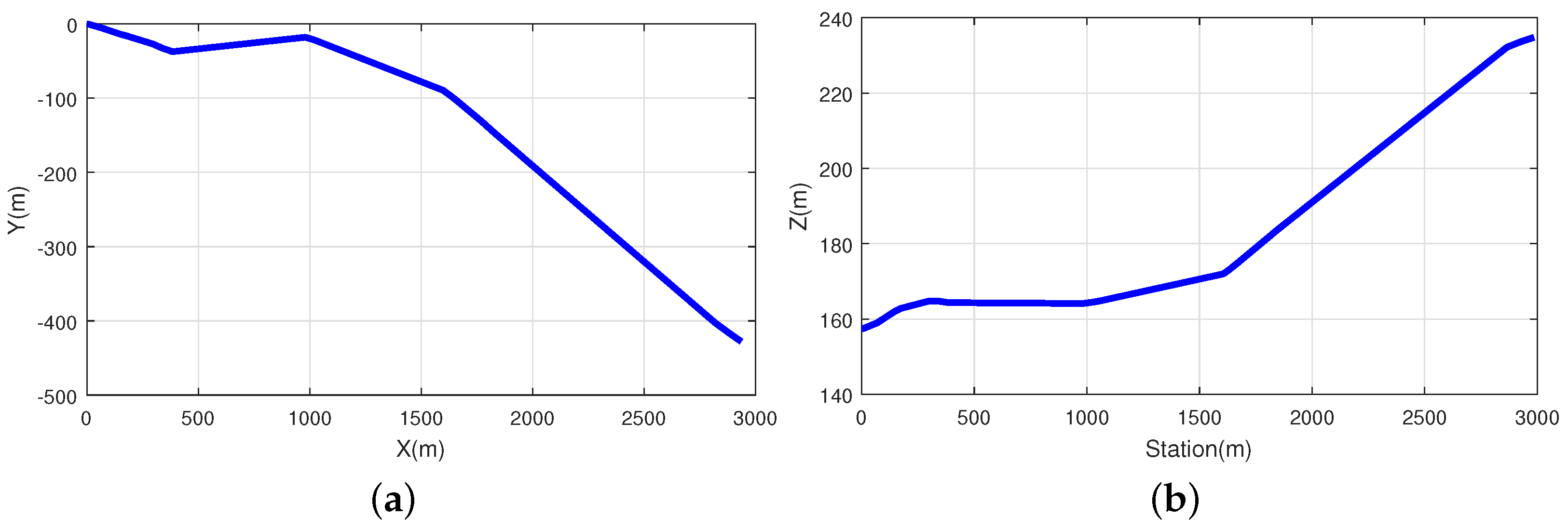
Maximal suspension deflection ($d_{max}$)	70	mm

. The simulation route is a highway based on real geographical and speed limit data, see Figure 8a and integrated to the TruckSim environment, see Figure 8b.

In order to demonstrate the effectiveness of the proposed method two different simulations have been performed and compared, one with the utility truck having conventional semi-active suspension and another with an adaptive semi-active suspension control. Note, that only a 3 km section of the route has been considered, with the road geometry shown in Figure 9b. The figures in this section have been plotted with the travel distance for the simulated vehicle and its performance results that were provided by Trucksim. 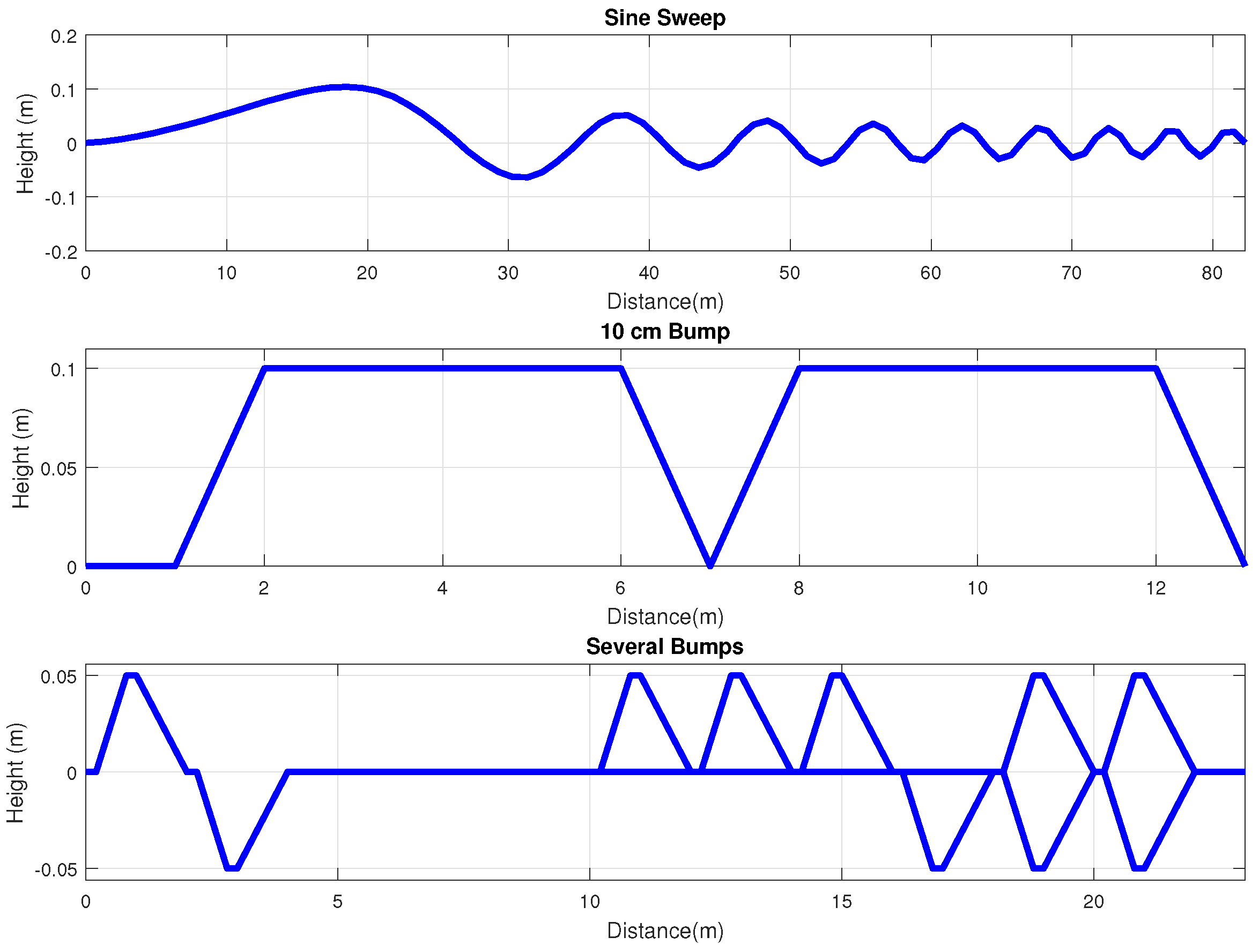As it is shown in Figure 9b, there are three major curves in the selected road section around 400 m, 1000 m and 1700 m. Moreover, there are also three different kinds of road irregularities to simulate different road distortion, see Figure 10. First, in 2 different locations in the road 200 m and 2200 m there are bumps and potholes following each other differently for the left to the right side of the lane, having a height and depth of 50 mm. This road type is a kind of road irregularity that represents the effect of driving over a speed bump, which is common in urban areas. Next, after in 2 different locations around 950 m and 2000 m, there are left and right side bumps following each other having 100 mm of height. This road irregularity represents bad road quality with discontinuities in the asphalt. Finally, at 2650 m there is a longitudinal sinusoidal road irregularity with growing frequency, putting extreme stress on the suspension system of the simulated vehicle. This kind of road surface is typical at bus stops, where the frequent braking of heavy road vehicles roll up the asphalt.

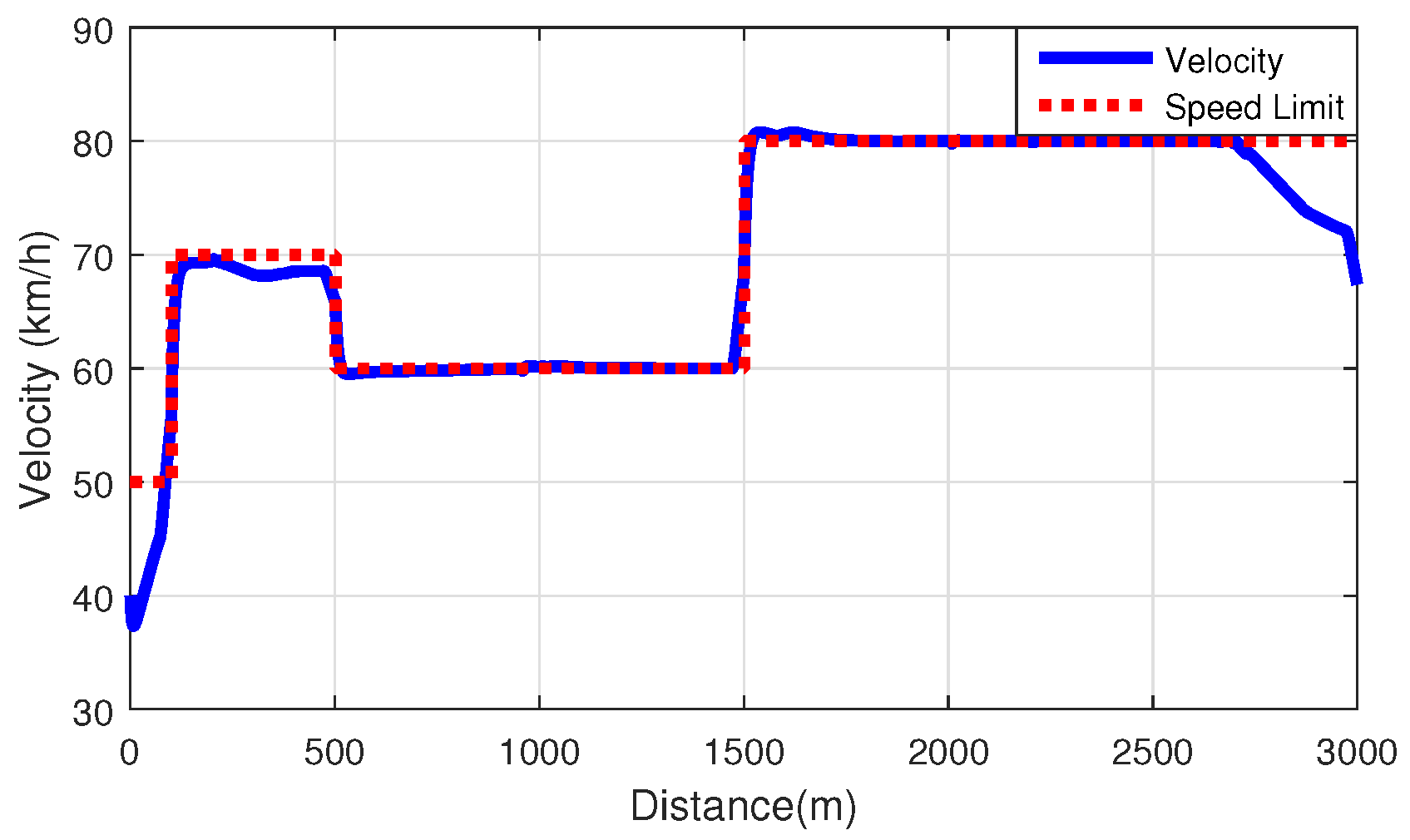
As shown in Figure 11, the real speed limit changes on the route, and both vehicles calculate its corresponding optimal velocity based on the energy-efficient look-ahead method. According to road distortions and velocity provided by the look-ahead controller, the decision layer selects a different value for the scheduling variable.

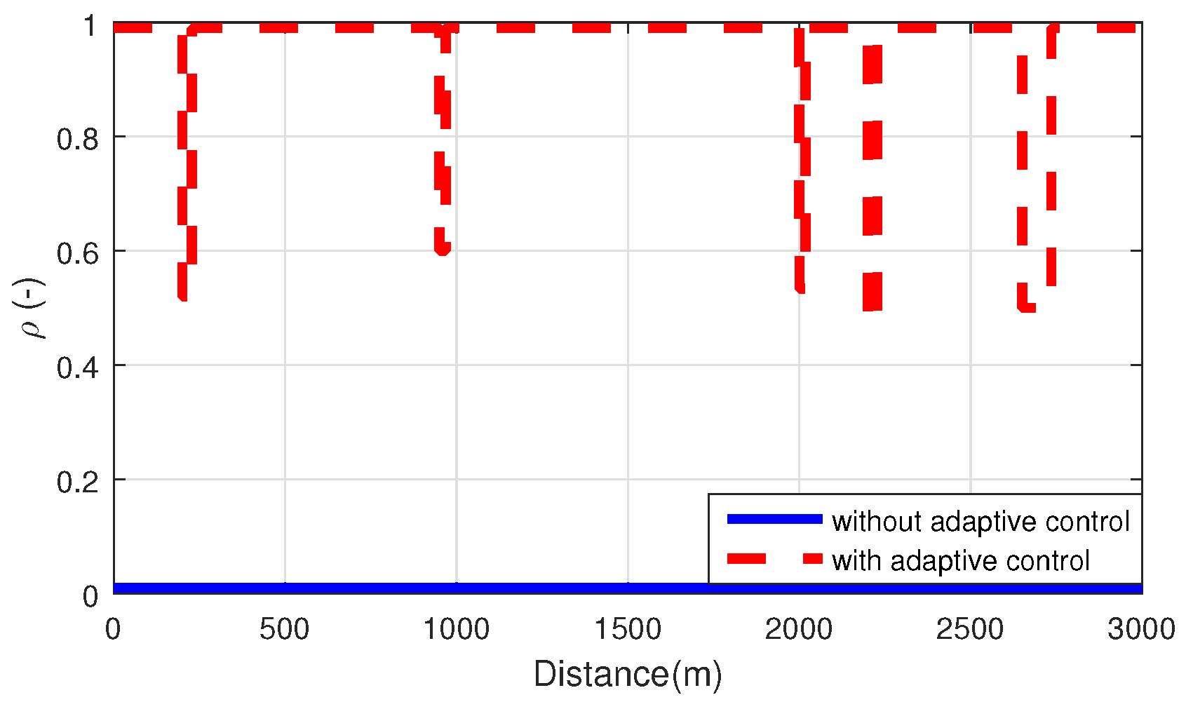
Figure 12 shows selected scheduling variable, where selection process was mentioned in Section 4 for the adaptive control simulation and constant scheduling variable for comparison. Selected $\rho \cong 0.52$ for the first several bumps at 200 m, $\rho \cong 0.6$ for the 10 cm bump at 950 m, $\rho \cong 0.54$ for the second 10 cm bump at 2000 m, $\rho \cong 0.47$ for second several bumps which is at 2200 m and for the sine sweep which is at 2650 m, $\rho \cong 0.5$.

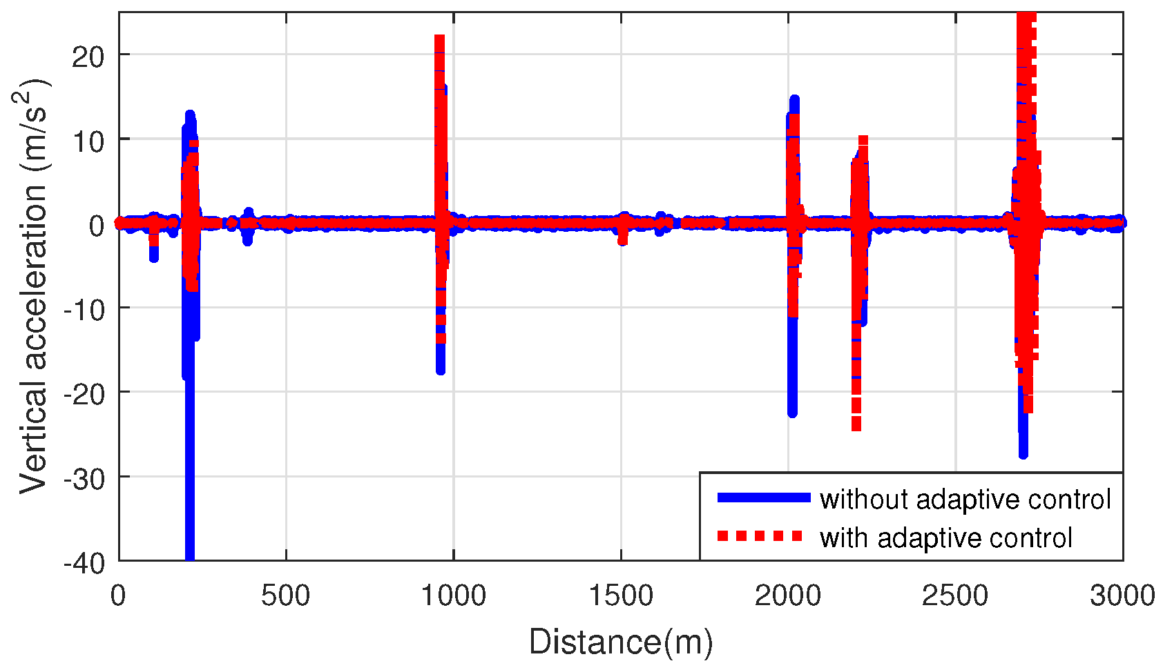
The performances are compared for the two simulated vehicles. In Figure 13 it can be seen that vertical acceleration performance has been improved both in flat road and at the road distortions. The biggest change is in the first several bumps distortion, while the change for the sine sweep road category between adaptive and non-adaptive control is not as significant. The reason for this phenomenon is that at the sine sweep road category scheduling variable is closer to zero.

Although longitudinal and lateral accelerations are not performances, these values also decreased with the introduced adaptive control, see Figure 14.

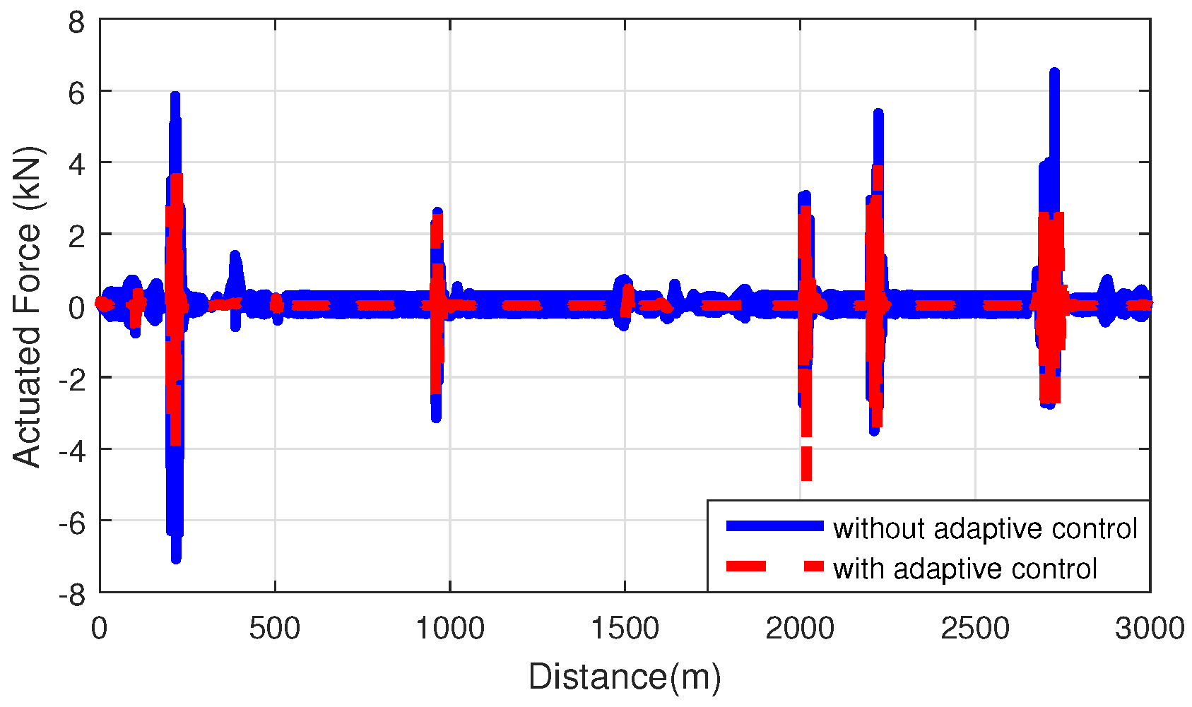
Another performance is to minimize actuated force for each damper in the semi-active suspension control design, while it is also needed to reduce actuated force in adaptive control. It is possible to see that actuated force is also decreased with adaptive semi-active suspension control. Figure 15 shows actuated force for the front left damper.

It has been shown that amount of the suspension deflection has been reduced with the introduced adaptive suspension system in both flat road and road distortions, see Figure 16, while the change at the flat road is smaller than at the road distortions. The biggest change in the suspension deflection is at the sine sweep road distortion for all four suspensions.

Although not as much as other performances, the amount of the tire deformation also has been decreased with the proposed adaptive suspension system at both flat road and road distortions, see Figure 17. There is a change at the several bumps and 10 cm bumps distortions, while the change at the sine sweep distortion cannot be seen. Here, the change in tire deformation of rear wheels is bigger for the whole road.

6. Conclusions

This paper proposed a new method with the integration of look-ahead road data in the control of the adaptive semi-active suspension, where it is possible to design a trade-off between comfort and stability with the decision layer. The model of the two-degree-of-freedom quarter-car model has been used for the modeling of the suspension system. The decision algorithm calculates the most efficient scheduling variable for the LPV controller by finding the best trade-off between riding comfort and vehicle safety. In the meantime, it proposes designing the vehicle velocity for the cruise controller by considering energy efficiency and comfort at the same time. The effectiveness of the proposed method has been validated in Trucksim environment with comparing two different simulations, one with conventional semi-active suspension control and another with an adaptive semi-active suspension control. The results of the simulations show that the performances of vertical acceleration, tire deformation and suspension deflection have been improved with the proposed adaptive suspension and cruise control system. Actuated forces have the greatest difference between these two methods and the smallest difference is in the tire deformation performance. A significant change in the acceleration performances is one of the evidence, which shows the introduced method is more efficient. Apart from all these, optimal velocity based on the energy-efficient look-ahead method follows the real speed limit, which changes on the route.

Future studies should aim to replicate results in more road categories and irregularities. Automated real-time road category detection and classification are also really important for similar researches, thus this assumption might be addressed in future studies.