Article

Adaptive Control for a Biological Process under Input Saturation and Unknown Control Gain via Dead Zone Lyapunov Functions

by
Alejandro Rincón
1,2,
Fredy E. Hoyos
3,* and
John E. Candelo-Becerra
4
1
Grupo de Investigación en Desarrollos Tecnológicos y Ambientales—GIDTA, Facultad de Ingenieria y Arquitectura, Universidad Católica de Manizales, Carrera 23 No. 60-63, Manizales 170002, Colombia
2
Grupo de Investigación en Microbiología y Biotecnología Agroindustrial—GIMIBAG, Instituto de Investigación en Microbiología y Biotecnología Agroindustrial, Universidad Católica de Manizales, Carrera 23 No. 60-63, Manizales 170002, Colombia
3
Facultad de Ciencias, Escuela de Física, Universidad Nacional de Colombia, Sede Medellín, Carrera 65 No. 59A, 110, Medellín 050034, Colombia
4
Departamento de Energía Eléctrica y Automática, Facultad de Minas, Universidad Nacional de Colombia, Sede Medellín, Carrera 80 No. 65-223, Robledo, Medellín 050041, Colombia
*
Author to whom correspondence should be addressed.
Appl. Sci. 2021, 11(1), 251; https://doi.org/10.3390/app11010251
Submission received: 27 November 2020 / Revised: 21 December 2020 / Accepted: 23 December 2020 / Published: 29 December 2020

Abstract

:
In this work, substrate control of a biological process with unknown varying control gain, input saturation, and uncertain reaction rate is addressed. A novel adaptive controller is proposed, which tackles the combined effect of input saturation and unknown varying control gain with unknown upper and lower bounds. The design is based on dead zone radially unbounded Lyapunov-like functions, with the state backstepping as control framework. The convergence of the modified tracking error and the boundedness of the updated parameters are ensured by means of the Barbalat’s lemma. As the first distinctive feature, a new second-order auxiliary system is proposed that tackles the effect of saturated input and the unknown varying control gain with unknown upper and lower bounds. As the second distinctive feature, the modified tracking error converges to a compact set whose width is user-defined, so that it does not depend on bounds of either external disturbances, model terms, or model coefficients. The convergence region of the current tracking error is determined for the closed loop system subject to the formulated controller and the proposed auxiliary system. Finally, numerical simulation illustrates the performance of the proposed controller.

1. Introduction

Automatic control of biological processes based on non-adaptive schemes is commonly affected by model uncertainty: (i) uncertain time varying coefficients of the reaction rates, (ii) uncertain time varying reaction yields, (iii) uncertain concentrations, and (iv) varying and uncertain or noisily measured inflow substrate concentration [1,2,3]. Adaptive control can achieve output stabilization despite these model uncertainties. Indeed, it can guarantee asymptotic convergence of the tracking error and boundedness of its updated parameters [4,5,6,7].
In addition to the effects of model uncertainty, control of biological process can be affected by actuator saturation in the case that integral action is used, for instance, the case with update laws [8,9]. Indeed, in adaptive control design, updated parameters may change excessively [10]. One strategy for tackling the effect of input saturation in control design of nonlinear systems is the augmented error signal (AES). In adaptive controllers with AES strategy, it is ensured that (i) closed loop signals are bounded and excessive increase of updated parameters is avoided and (ii) the modified tracking error asymptotically converges to a compact set of small size [10,11,12]. An early incorporation of the AES strategy to Lyapunov-based adaptive control is presented in [10]. The tracking error signal is substituted by the modified tracking error, which is the sum of the tracking error and a filter in terms of the input error Δ u , which is the difference between the constrained and unconstrained input signals [10,11,12]. In the case of high order nonlinear systems, the backstepping strategy is commonly used, and the auxiliary system is defined as a nth order filter in terms of Δ u [11,12,13].
In adaptive backstepping control design, the input saturation is usually tackled by using the AES strategy [12,14]. However, accounting for unknown varying control gain is not common in these designs. In [12], a general nonlinear time-delay system of nth order is considered, and an output feedback backstepping is designed. Moreover, the model of a two-stage chemical reactor with recirculation is considered as a second-order particular case. However, the controller design assumes the control gain as constant and perfectly known. In [15], a CSTRconsisting of a second-order SISO model is considered, in which only the output is known. The used anti-windup compensator amounts to the auxiliary system of the AES strategy. However, the controller design assumes that the control gain is perfectly known. In [14], a nth order system with unknown nonlinear control gain is considered. The unknown nonlinear nature of the control gain is tackled by using the Nussbaum gain strategy. However, the width of the convergence region of the modified tracking error depends on unknown model coefficients and terms. In summary, in the aforementioned AES-based robust adaptive backstepping control designs, the modified tracking error converges to a compact set whose width depends on the bounds of either external disturbances, model terms or model parameters [11,12,14]. This implies that such bounds must be known to achieve a user-defined magnitude of the steady value of the modified tracking error.
In this study, a modified/new robust adaptive backstepping controller is developed for a second-order SISO nonlinear system, tackling the effect of input saturation and unknown varying control gain with unknown upper and lower bounds. The design is based on dead zone radially unbounded forms, and a new auxiliary system is proposed. The asymptotic convergence of the modified tracking error is proved by using the Barbalat’s lemma, accounting for the unknown varying control gain, the saturated input, and the formulated controller. It is ensured that the regular tracking error converges to a residual set of user-defined width, for the case that the input saturation eventually ceases. The main contributions of this study with respect to adaptive backstepping control designs for systems with input saturation are listed below.
  • The proposed auxiliary system is robust against varying and unknown control gain with unknown upper and lower bounds. This is in contrast to common adaptive backstepping control designs (see in [12,15]) where the auxiliary system considers the control gain as constant and unknown.
  • The modified tracking error converges to a compact set whose width is user-defined, so that it does not depend on the bounds of either external disturbances, model terms, system states, or model parameters. This is in contrast to common adaptive backstepping control designs (see in [12,15]) and also those that use the Nussbaum gain strategy (see in [14]) where the width of the convergence region of the modified tracking error depends on such kind of bounds.
  • The convergence region of the tracking error is determined for the closed loop system under the formulated controller with the proposed auxiliary system.
The work is organized as follows. In Section 2, the model of the biological process, the reference model, and the statement of the control goal are presented. In Section 3, the controller is designed and the stability properties of the closed loop states are determined. In Section 4, a simulation example is presented. In Section 5, the conclusions are drawn.

2. Model Description, Reference Model and Control Goal

2.1. Model Description

The second order nonlinear SISO model of an hydroponic culture described in Appendix A is
d x 1 d t = a 1 x 2 a 2 x 1 r x 1
d x 2 d t = a 3 1 x 3 ( x 1 x 2 ) + a 4 x 3 x 2 + b v
d x 3 d t = Q e Q i Q l o s s + v
where
b = P a d x 2 x 3 , a 1 = Q i / V u , a 2 = Q e / V u , a 3 = Q e , a 4 = Q l o s s x 1 = P e , x 2 = P i , x 3 = V l , v = Q a d ,
P e is the nutrient concentration in the upper CSTR, P i is the nutrient concentration in the lower CSTR, V l is the volume of the lower CSTR, V u is the volume of the upper CSTR, and Q e is the flow that leaves the upper CSTR and enters the lower CSTR; Q i is the flow that leaves the lower CSTR and enters the upper CSTR; Q a d is the flow of addition of fresh nutrient solution to the mixing tank; and P a d is the nutrient concentration of the Q a d flow. The state x 1 is the output to be controlled, whereas the inlet flowrate Q a d is chosen as control input, it is non-negative and its upper bound is determined by the operational limit of the pump. Therefore, the relationship between the constrained control signal (denoted as v) and the unconstrained control signal (denoted as u) is
v = u m a x if u > u m a x u if u [ u m i n u m a x ] u m i n if u < u m i n
The following assumptions are considered:
Assumption 1.
The state variables x 1 and x 2 , x 3 are bounded for v bounded, and satisfy x 1 R + , x 2 R + , x 3 R + .
Assumption 2.
a 1 , a 2 , a 3 , a 4 are constant, a 2 , a 3 , a 4 are unknown whereas a 1 is known.
Assumption 3.
The reaction rate r x 1 satisfies one of the following: (i) it is unknown, non-negative, and r x 1 μ ¯ 1 r ¯ x 1 , where μ ¯ 1 is unknown, positive, constant, whereas r ¯ x 1 is a known continuous function of x 1 with well-defined d r ¯ x 1 / d x 1 ; (ii) it is a known continuous function of x 1 , with well-defined d r x 1 / d x 1 ; in this case, r x 1 = μ ¯ 1 r ¯ x 1 with r ¯ x 1 = r x 1 , μ ¯ 1 = 1 holds true.
Assumption 4.
The values of x 1 , x 2 are known, whereas x 3 is noisily measured: x 3 m = x 3 + δ x 3 , where x 3 m is the noisy measurement and δ x 3 is the measurement noise.
Assumption 5.
There is lack of knowledge on the control gain b according to one of the following conditions: (i) b = b δ b m , where b m is known, and possibly varying, and bounded for x 1 , x 2 , x 3 bounded, whereas b δ is unknown, varying, and satisfies: μ ¯ l b | b δ | μ ¯ u b , where μ ¯ l b , μ ¯ u b are constant, positive and unknown; (ii) b is unknown, varying, and satisfies μ ¯ l b | b | μ ¯ u b , where μ ¯ l b , μ ¯ u b are unknown positive constants; in this case, b can be expressed as b = b δ b m , b m = 1 , b δ = b , so that b δ is unknown, varying and satisfies μ ¯ l b | b δ | μ ¯ u b . In both conditions, b = b δ b m , where b m is known, whereas b δ is unknown, varying and satisfies μ ¯ l b | b δ | μ ¯ u b ; so that | b | μ ¯ u b | b m | .

2.2. Reference Model

The use of a reference model allows to obtain the expected transient plant response (rise time, settling time, overshoot). The reference model is defined as [16,17]
y d = a m 1 / 2 ( p + a m 1 / 2 ) a m 1 / 2 ( p + a m 1 / 2 ) W r e f
where y d is the desired output; W r e f is the command signal, which is user-defined and bounded; a m is a positive constants defined by the user, which determine the speed of convergence of the signal y d towards W r e f ; and p = d / d t is the differential operator. Due to the above characteristics, the signals y d , y ˙ d , y ¨ d are bounded and known. The reference model (5) can be rewritten as
d 2 y d d t 2 + a m 1 d y d d t + a m 1 2 4 y d = a m 1 2 4 W r e f
or, equivalently,
d y d d t = a m 1 2 y d + a m 1 2 y d o d y d o d t = a m 1 2 y d o + a m 1 2 W r e f

2.3. Control Goal

Consider (i) the plant model (1) to (3), subject to input constraint (4) and Assumptions 1 to 5; (ii) the tracking error e = x 1 y d , where x 1 is the output, and y d is the desired output, whose characteristics are mentioned in Section 2.2; (iii) the residual set Ω e o = { e : | e | C b } , whose width C b is positive, constant and user-defined. The goal of the controller design is to formulate a control law for v such that (Gi) the tracking error e converges asymptotically to the residual set Ω e o , (Gii) the control law and the update laws are bounded under closed loop operation, so that excessive parameter increase is avoided; (Giii) the control law, the update law and the auxiliary system involve no discontinuous signals.
Remark 1.
The condition Giii is stated because the presence of discontinuous signals in the control law may lead to input chattering, and problems of existence and uniqueness of closed loop trajectories, and consequently, Filippov theory is needed, as discussed in [18,19].

3. Control Design and Stability Analysis

In this section, the proposed robust adaptive controller is developed for the model described in Section 2, which involves input constraint, unknown varying control gain, and unknown model parameters.

3.1. Controller Design

The controller design uses Lyapunov theory, with the adaptive backstepping strategy as framework. New states z 1 and z 2 are defined as function of x 1 , x 2 , and updated parameters. Furthermore, an overall Lyapunov function V is defined as the sum of V z 1 , the dead zone Lyapunov function for z 1 ; V z 2 , the dead zone Lyapunov function for z 2 ; and a Lyapunov function for each parameter updating error. Differential equations are defined for the new states, and the time derivatives of the Lyapunov functions are defined. The mechanisms for the updated parameters and the control input u are chosen such that d V / d t is negative semi-definite, thus implying the asymptotic convergence of z 1 . Other important features of the developed procedure are
  • a new auxiliary system of second order is proposed, whose input includes the control signal error Δ u , which is the difference between the constrained and the unconstrained control signals;
  • a modified tracking error z 1 is defined as the sum of the regular tracking error and the state of the auxiliary system;
  • the definition the z i states is based on the adaptive state backstepping method;
  • dead zone radially unbounded quadratic forms are used instead of current quadratic forms; and
  • a new treatment of the b Δ u term is proposed, including a new parameterization of the unknown model parameters, and the formulation of a new auxiliary system.
In a basic adaptive backstepping control design, the z 1 state would be defined as the tracking error, z 1 = x 1 y d . In contrast, we define z 1 by adding ψ 1 to the tracking error:
z 1 = x 1 y d ψ 1
where the ψ 1 state is the output of a stable second order linear filter whose input contains the input error Δ u , the difference between the non-saturated and the saturated input signals. The controller design is aimed at driving z 1 to Ω z 1 , Ω z 1 = z 1 : | z 1 | C b . The advantages of the definition of z 1 (6) and the controller design based on z 1 instead of the tracking error e are (i) excessive increase of the updated parameters is avoided and (ii) the convergence region of the tracking error e = x 1 y d in presence of input saturation can be determined. The time derivative of Equation (6) is
z ˙ 1 = x ˙ 1 y ˙ d ψ ˙ 1
Incorporating the x ˙ 1 expression (1) yields
z ˙ 1 = a 1 x 2 a 2 x 1 r x 1 y ˙ d ψ ˙ 1
Let
V z 1 = ( 1 / 3 ) ( z 1 C b ) 3 for z 1 C b 0 for z 1 ( C b , C b ) ( 1 / 3 ) ( 1 ) ( z 1 + C b ) 3 for z 1 C b
This truncated Lyapunov function is inspired on that of [20,21]. Early versions of dead zone Lyapunov functions are presented in [17,22,23]; versions for backstepping-based controllers in [21,24], and other versions in [20,25,26]. The use of the dead zone Lyapunov function (9) allows designing the adaptive controller, tackling the presence of unknown varying terms or parameters, and avoiding the use of discontinuous signals. The main properties of V z 1 (9) are
V z 1 = 0 for z 1 [ C b , C b ] V z 1 > 0 for z 1 [ C b , C b ] V z 1 is continuous with respect to z 1 , and it is bounded for z 1 bounded
The above properties and a stable dynamics of V z 1 imply the convergence of z 1 to Ω z 1 , Ω z 1 = z 1 : | z 1 | C b , as is shown in the convergence theorem in Section 3.2.
Differentiating (9) with respect to time yields
V ˙ z 1 = f z 1 z ˙ 1
f z 1 = d V z 1 d z 1 = ( z 1 C b ) 2 for z 1 C b 0 for z 1 ( C b , C b ) ( 1 ) ( z 1 + C b ) 2 for z 1 C b
Incorporating the expression for z ˙ 1 (8) into Equation (10) and arranging yields
V ˙ z 1 = k 1 b | f z 1 | k 1 f z 1 2 + f z 1 a 1 x 2 + f z 1 k 1 f z 1 y ˙ d ψ ˙ 1 a 2 x 1 r x 1 + k 1 b s i g n ( f z 1 )
where k 1 b | f z 1 | was incorporated in order to provide robustness and | f z 1 | was expressed as | f z 1 | = f z 1 s i g n ( f z 1 ) , which would imply the presence of the signal s i g n ( f z 1 ) in the definition of z 2 and would hamper the determination of z ˙ 2 . Thus, notice that from the definition of f z 1 (11) it follows that
| f z 1 | = f z 1 s a t z 1 where
s a t z 1 = z 1 C b 2 | z 1 | C b for z 1 ( C b , C b ) s g n ( z 1 ) otherwise
d s a t z 1 d z 1 = 2 C b 1 | z 1 | C b for z 1 ( C b , C b ) 0 otherwise
Using (13) in (12) instead of | f z 1 | = f z 1 s i g n ( f z 1 ) , yields
V ˙ z 1 = k 1 b | f z 1 | k 1 f z 1 2 + f z 1 a 1 x 2 + f z 1 k 1 f z 1 y ˙ d ψ ˙ 1 a 2 x 1 r x 1 + k 1 b s a t z 1
To obtain the required right hand side of d V z 1 / d t , the effect of the term f z 1 a 1 x 2 + f z 1 k 1 f z 1 y ˙ d ψ ˙ 1 a 2 x 1 r x 1 + k 1 b s a t z 1 should be tackled by adequate definition of the new state z 2 . However, a 2 is unknown and r x 1 is unknown, and its upper bound comprises and unknown constant μ ¯ 1 . Therefore, the term f z 1 ( a 2 x 1 r x 1 ) should be expressed in terms of updated parameters and parameter estimation error. Recall from Assumption 3 that r x 1 μ ¯ 1 r ¯ x 1 or r x 1 = μ ¯ 1 r ¯ x 1 , therefore
f z 1 ( r x 1 ) μ ¯ 1 r ¯ x 1 | f z 1 |
The term f z 1 ( a 2 x 1 r x 1 ) can be parameterized accounting for (17) and (13):
f z 1 ( a 2 x 1 r x 1 ) φ 1 θ 1 f z 1
φ 1 = [ x 1 , s a t z 1 r ¯ x 1 ] , θ 1 = [ a 2 , μ ¯ 1 ]
As the parameter vector θ 1 is unknown, we express it in terms of an updated parameter vector and a parameter updating error as follows. Let θ ˜ 1 = θ ^ 1 θ 1 , where θ ˜ 1 , θ ^ 1 are the parameter estimation error and the updated parameter, being θ ^ 1 provided by an updating mechanism defined later. Thus, θ 1 can be expressed as θ 1 = θ ^ 1 θ ˜ 1 . Substituting into Equation (18) yields f z 1 ( a 2 x 1 r x 1 ) φ 1 θ ^ 1 f z 1 φ 1 θ ˜ 1 f z 1 . Substituting this into Equation (16) yields
V ˙ z 1 k 1 b | f z 1 | k 1 f z 1 2 + f z 1 a 1 x 2 + f z 1 φ 1 θ ^ 1 + k 1 f z 1 y ˙ d ψ ˙ 1 + k 1 b s a t z 1 φ 1 θ ˜ 1 f z 1
The dynamics of V z 1 is affected by the following terms: (i) the term k 1 b | f z 1 | k 1 f z 1 2 is negative and it provides stability; (ii) the term φ 1 θ ˜ 1 f z 1 , which is later tackled by defining a quadratic form for θ ˜ 1 , as can be noticed in the boundedness and convergence theorems in Section 3.2; and (iii) the term f z 1 a 1 x 2 + f z 1 φ 1 θ ^ 1 + k 1 f z 1 y ˙ d ψ ˙ 1 + k 1 b s a t z 1 , which is later tackled by adequate definition of the new state z 2 , so that this term equals f z 1 z 2 and (20) yields
V ˙ z 1 k 1 b | f z 1 | k 1 f z 1 2 + f z 1 z 2 φ 1 θ ˜ 1 f z 1 where
z 2 = a 1 x 2 + ( k 1 f z 1 y ˙ d ψ ˙ 1 ) + k 1 b s a t z 1 + φ 1 θ ^ 1
The effect of the term f z 1 z 2 can be tackled by adequate dynamics of V z 1 and V z 2 , such that V ˙ z 1 + V ˙ z 2 involves the term k f z 1 2 k f z 2 2 , being f z 2 a saturation function of z 2 and V z 2 a quadratic function of f z 2 . To this end, the required dynamics of z 2 is generated next.
Differentiating z 2 (22) with respect to time yields
z ˙ 2 = a 1 x ˙ 2 + k 1 d f z 1 d z 1 z ˙ 1 y ¨ d ψ ¨ 1 + k 1 b d s a t z 1 d z 1 z ˙ 1 + φ ˙ 1 θ ^ 1 + φ 1 θ ^ ˙ 1
The auxiliary state ψ 1 and its time derivatives are provided by the auxiliary system, whose general structure consists of a second order linear filter whose input W ψ involves the input error Δ u :
ψ ˙ 1 = K ψ 1 ψ 1 + ψ 2
ψ ˙ 2 = K ψ 2 ψ 2 + W ψ
where the term W ψ , which will be defined later, is used to cancel the effect of the Δ u term, which is the difference between the saturated and non-saturated input signals. From (24), (25) it follows that ψ ¨ 1 = K ψ 1 2 ψ 1 ( K ψ 1 + K ψ 2 ψ 2 ) + W ψ . Substituting this expression and the expressions for z ˙ 1 (7), x ˙ 1 (1) and x ˙ 2 (3) into Equation (23) and arranging yields
z ˙ 2 = k 2 f z 2 + a 1 a 3 x 1 x 2 x 3 + a 1 a 4 x 2 x 3 + B 1 d ( a 2 x 1 r x 1 ) + B 1 e + a 1 b v + ( 1 ) W ψ
where
B 1 d = k 1 d f z 1 d z 1 + k 1 b d s a t z 1 d z 1 + B 1 b
B 1 e = B 1 d a 1 x 2 + k 1 d f z 1 d z 1 + k 1 b d s a t z 1 d z 1 ( 1 ) ( y ˙ d + ψ ˙ 1 ) + ( 1 ) K ψ 1 2 ψ 1 + ( K ψ 1 + K ψ 2 ) ψ 2 + B 10 + φ θ ^ ˙ 1 + k 2 f z 2 B 1 b = ( 1 ) θ ^ 1 , 1 + s a t z 1 d r ¯ x 1 d x 1 θ ^ 1 , 2 + r ¯ x 1 d s a t z 1 d z 1 θ ^ 1 , 2 B 10 = r ¯ x 1 d s a t z 1 d z 1 y ˙ d ψ ˙ 1 θ ^ 1 , 2 where d f z 1 d z 1 = 2 ( z 1 C b ) for z 1 C b 0 for z 1 ( C b , C b ) ( 2 ) ( z 1 + C b ) for z 1 C b
and d s a t z 1 / d z 1 is defined in Equation (15). Let
V z = V z 1 + V z 2
V z 2 = ( 1 / 2 ) ( z 2 C b ) 2 for z 2 C b 0 for z 2 ( C b , C b ) ( 1 / 2 ) ( z 2 + C b ) 2 for z 2 C b
The main properties of V z 2 are
V z 2 = 0 for z 2 [ C b , C b ] V z 2 > 0 for z 2 [ C b , C b ] V z 2 is continuous with respect to z 2 , and it is bounded for z 2 bounded
The above properties and a stable dynamics of V z 2 imply the convergence of z 2 to Ω z 2 , Ω z 2 = z 2 : | z 2 | C b , as shown in the convergence theorem in Section 3.2.
Differentiating V z 2 with respect to time yields
V ˙ z 2 = f z 2 d z 2 d t ,
f z 2 = d V z 2 d z 2 = z 2 C b for z 2 C b 0 for z 2 ( C b , C b ) z 2 + C b for z 2 C b
Incorporating the expression for z ˙ 2 (26) into Equation (31) and arranging yields
V ˙ z 2 = k 2 f z 2 2 + f z 2 a 1 a 3 x 1 x 2 x 3 + a 1 a 4 x 2 x 3 + B 1 d ( a 2 x 1 r x 1 ) + B 1 e + f z 2 a 1 b v + ( 1 ) W ψ
Differentiating V z in (29) with respect to time yields V ˙ z = V ˙ z 1 + V ˙ z 2 . Substituting the expressions for V ˙ z 1 (21) and V ˙ z 2 (33) yields
V ˙ z C b | f z 1 | + f z 1 z 2 k 1 f z 1 2 k 2 f z 2 2 φ 1 θ ˜ 1 f z 1 + f z 2 a 1 a 3 x 1 x 2 x 3 + a 1 a 4 x 2 x 3 + B 1 d ( a 2 x 1 r x 1 ) + B 1 e + f z 2 a 1 b v + ( 1 ) W ψ
To obtain the required right hand side of d V z / d t , the terms
f z 1 z 2 + f z 2 a 1 a 3 x 1 x 2 x 3 + a 1 a 4 x 2 x 3 + B 1 d ( a 2 x 1 r x 1 ) + B 1 e
should be rewritten and tackled by means of proper definition of W ψ and the control law.
In the f z 1 z 2 term, the z 2 signal must be expressed in terms of f z 2 , because the controller design is based on the dead zone functions f z 1 and f z 2 rather than z 1 and z 2 . From definition (32), it follows that f z 2 = z 2 + δ ,
δ = C b for z 2 C b 0 for z 2 ( C b , C b ) C b for z 2 C b
therefore, z 2 = f z 2 δ and | δ | C b . Therefore, f z 1 z 2 = f z 1 f z 2 δ f z 1 . Substituting into Equation (34) yields
V ˙ z C b | f z 1 | δ f z 1 k 1 f z 1 2 k 2 f z 2 2 φ 1 θ ˜ 1 f z 1 + f z 2 f z 1 + a 1 a 3 x 1 x 2 x 3 + a 1 a 4 x 2 x 3 + B 1 d ( a 2 x 1 r x 1 ) + B 1 e + f z 2 a 1 b v + ( 1 ) W ψ
so that the error term δ leads to the undesired uncertainty term δ f z 1 in Equation (35). The property | δ | C b implies that δ f z 1 C b | f z 1 | , which is canceled by the already existing term C b | f z 1 | , so that C b | f z 1 | δ f z 1 0 , and Equation (35) yields
V ˙ z k 1 f z 1 2 k 2 f z 2 2 φ 1 θ ˜ 1 f z 1 + f z 2 f z 1 + a 1 a 3 x 1 x 2 x 3 + a 1 a 4 x 2 x 3 + B 1 d ( a 2 x 1 r x 1 ) + B 1 e + f z 2 a 1 b v + ( 1 ) W ψ
Therefore, the term C b | f z 1 | incorporated in Equation (12) is necessary for counteracting the effect of the error term δ resulting from f z 2 = z 2 + δ .
In order to facilitate the design of the control law for u, the constrained input signal v is expressed in terms of the unconstrained input signal u and the input error Δ u , and the effect of Δ u is later canceled by the input of the auxiliary system, W ψ . Let
Δ u = v u hence
v = u + Δ u
Substituting (38) into (36), yields
V ˙ z k 1 f z 1 2 k 2 f z 2 2 φ 1 θ ˜ 1 f z 1 + f z 2 f z 1 + a 1 a 3 x 1 x 2 x 3 + a 1 a 4 x 2 x 3 + B 1 d ( a 2 x 1 r x 1 ) + B 1 e + a 1 f z 2 b u + a 1 f z 2 b Δ u + f z 2 ( 1 ) W ψ
The effect of the term a 1 f z 2 b Δ u should be canceled by an adequate choice of W ψ , but this is hampered by the uncertainty on the control gain b. To this end, b is expressed in terms of an updated parameter and a parameter updating error. Recall from assumption 5 that | b | μ ¯ u b | b m | . Therefore,
a 1 f z 2 b Δ u μ u b a 1 | f z 2 b m Δ u |
As the upper bound μ ¯ u b is unknown, it is expressed in terms of updated parameter and parameter updating error. Let θ ˜ u b = θ ^ u b μ ¯ u b , where θ ˜ u b , θ ^ u b are a parameter estimation error and an updated parameter, and θ ^ u b is provided by an updating mechanism defined later. From the above definition it follows that μ ¯ u b = θ ^ u b θ ˜ u b . Substituting into Equation (40) and arranging, yields
a 1 f z 2 b Δ u θ ^ u b a 1 | f z 2 b m Δ u | a 1 | f z 2 b m Δ u | θ ˜ u b
Substituting into Equation (39), yields
V ˙ z k 1 f z 1 2 k 2 f z 2 2 φ 1 θ ˜ 1 f z 1 + f z 2 f z 1 + a 1 a 3 x 1 x 2 x 3 + a 1 a 4 x 2 x 3 + B 1 d ( a 2 x 1 r x 1 ) + B 1 e + a 1 f z 2 b u + θ ^ u b a 1 | f z 2 b m Δ u | a 1 | f z 2 b m Δ u | θ ˜ u b + f z 2 ( 1 ) W ψ
Thus, the right hand side of d V z / d t is affected by the following terms: (i) the term θ ^ u b a 1 | f z 2 b m Δ u | , which is later tackled by properly choosing W ψ , and (ii) the term a 1 | f z 2 b m Δ u | θ ˜ u b , which is later tackled by defining the quadratic form for θ ˜ u b . To this end, if | f z 2 | is expressed as | f z 2 | = f z 2 s i g n ( f z 2 ) , the resulting expression of W ψ would contain the s i g n ( f z 2 ) signal, so that chattering might occur. Therefore, we notice from definition (32) that
| f z 2 | = f z 2 s a t z 2 where
s a t z 2 = + 1 for z 2 C b ( 1 / C b ) z 2 for z 2 ( C b , C b ) 1 for z 2 C b
Therefore, (41) leads to
a 1 f z 2 b Δ u + f z 2 ( 1 ) W ψ f z 2 θ ^ u b s a t z 2 a 1 | b m Δ u | W ψ a 1 | f z 2 b m Δ u | θ ˜ u b
we choose
W ψ = a 1 θ ^ u b s a t z 2 | b m Δ u |
substituting into Equation (24), (25) gives the auxiliary system
ψ ˙ 1 = K ψ 1 ψ 1 + ψ 2
ψ ˙ 2 = K ψ 2 ψ 2 + a 1 θ ^ u b s a t z 2 | b m Δ u |
K ψ 1 > 1 / 2 , K ψ 2 > 1 / 2
where s a t z 2 is defined in (44). Substituting (46) into Equation (45) yields a 1 f z 2 b Δ u + f z 2 ( 1 ) W ψ a 1 | f z 2 b m Δ u | θ ˜ u b . Substituting this into (42) gives
V ˙ z k 1 f z 1 2 k 2 f z 2 2 φ θ ˜ 1 f z 1 + f z 2 a 1 a 3 x 1 x 2 x 3 + a 1 a 4 x 2 x 3 + B 1 d ( r x 1 a 2 x 1 ) + f z 1 + B 1 e + a 1 f z 2 b δ b m u | a 1 f z 2 b m Δ u | θ ˜ u b
The term
f z 2 a 1 a 3 x 1 x 2 x 3 + a 1 a 4 x 2 x 3 + B 1 d ( r x 1 a 2 x 1 ) + f z 1 + B 1 e
should be canceled by the input signal u appearing in the term a 1 f z 2 b δ b m u , but this is hampered by the lack of knowledge on (i) a 3 , μ l b , a 4 , a 2 and (ii) the control gain term b δ and its lower bound μ ¯ l b . Therefore, we need to express these terms as function of b δ , updated parameters and parameter updating errors. To begin, the term comprising x 1 x 2 can be expressed as
f z 2 a 1 a 3 x 1 x 2 x 3 μ l b a 1 | f z 2 ( x 1 x 2 ) | x 3 m θ 3 , θ 3 = a 3 μ l b 1 + m a x ( δ x 3 ) m i n ( x 3 )
Let θ ˜ 3 = θ ^ 3 θ 3 , where θ ˜ 3 and θ ^ 3 are a parameter updating error and an updated parameter, respectively, and θ ^ 3 is provided by an updating mechanism defined later. From the above definition it follows that θ 3 can be expressed as θ 3 = θ ^ 3 θ ˜ 3 . Substituting into Equation (49) and using property μ l b | b δ | from Assumption 5, yields
f z 2 a 1 a 3 x 1 x 2 x 3 a 1 | b δ f z 2 ( x 1 x 2 ) | x 3 m θ ^ 3 μ l b a 1 | f z 2 ( x 1 x 2 ) | x 3 m θ ˜ 3
In a similar way
f z 2 a 1 a 4 x 3 x 2 a 1 | b δ x 2 f z 2 | x 3 m θ ^ 4 μ l b a 1 | x 2 f z 2 | x 3 m θ ˜ 4 where θ ˜ 4 = θ ^ 4 θ 4
f z 2 B 1 d ( r x 1 ) | b δ f z 2 B 1 d | r ¯ x 1 θ ^ r x 1 μ l b | f z 2 B 1 d | r ¯ x 1 θ ˜ r x 1 where θ ˜ r x 1 = θ ^ r x 1 θ r x 1
f z 2 B 1 d ( a 2 x 1 ) | b δ f z 2 B 1 d x 1 | θ ^ 2 μ l b | f z 2 B 1 d x 1 | θ ˜ 2 where θ ˜ 2 = θ ^ 2 θ 2
f z 2 ( f z 1 + B 1 e ) | b δ f z 2 ( f z 1 + B 1 e ) | θ ^ i l b μ l b | f z 2 ( f z 1 + B 1 e ) | θ ˜ i l b where θ ˜ i l b = θ ^ i l b 1 / μ l b
Notice that the expressions (50)–(54) contain | f z 2 | . If it is expressed as | f z 2 | = f z 2 s i g n ( f z 2 ) , the resulting control law would contain the s i g n ( f z 2 ) signal, so that input chattering might occur. Thus, we use the expression (43), so that
| b δ f z 2 | = b δ f z 2 s g n ( b δ ) s a t z 2
Substituting (50)–(54) into Equation (48) and using (55), yields
V ˙ z k 1 f z 1 2 k 2 f z 2 2 φ 1 θ ˜ 1 f z 1 + b δ f z 2 s g n ( b δ ) s a t z 2 a 1 | x 1 x 2 | x 3 m θ ^ 3 + a 1 x 2 x 3 m θ ^ 4 + | B 1 d | r ¯ x 1 θ ^ r x + | B 1 d x 1 | θ ^ 2 + | f z 1 + B 1 e | θ ^ i l b + a 1 b m u μ l b | f z 2 | a 1 | x 1 x 2 | x 3 m θ ˜ 3 μ l b a 1 | f z 2 | | x 2 | x 3 m θ ˜ 4 μ l b | f z 2 B 1 d | r ¯ x 1 θ ˜ r x 1 μ l b | f z 2 B 1 d x 1 | θ ˜ 2 μ l b | f z 2 ( f z 1 + B 1 e ) | θ ˜ i l b | a 1 f z 2 b m Δ u | θ ˜ u b
Thus, the right hand side of d V z / d t is affected by the following terms: (i) the term k 1 f z 1 2 k 2 f z 2 2 which leads to convergence of f z 1 2 and f z 2 2 to zero, as shown in the convergence theorem in Section 3.2; (ii) the terms involving θ ˜ 1 , θ ˜ 3 , θ ˜ 4 , θ ˜ r x 1 , θ ˜ 2 , θ ˜ i l b , θ ˜ u b , which are later tackled by properly defining their quadratic forms and the update laws, what is shown later in the analysis of d V / d t ; and (iii) the remaining term
b δ f z 2 s g n ( b δ ) s a t z 2 a 1 | x 1 x 2 | x 3 m θ ^ 3 + a 1 x 2 x 3 m θ ^ 4 + | B 1 d | r ¯ x 1 θ ^ r x + | B 1 d x 1 | θ ^ 2 + | f z 1 + B 1 e | θ ^ i l b
which is tackled by properly defining the control law, so that the u signal cancels it:
b δ f z 2 s g n ( b δ ) s a t z 2 a 1 | x 1 x 2 | x 3 m θ ^ 3 + a 1 x 2 x 3 m θ ^ 4 + | B 1 d | r ¯ x 1 θ ^ r x + | B 1 d x 1 | θ ^ 2 + | f z 1 + B 1 e | θ ^ i l b + a 1 b m u = 0
Solving (57) for u yields
u = 1 b m a 1 s g n ( b δ ) s a t z 2 a 1 | x 1 x 2 | x 3 m θ ^ 3 + | B 1 d | r ¯ x 1 θ ^ r x 1 + | B 1 d x 1 | θ ^ 2 + | f z 1 + B 1 e | θ ^ i l b + a 1 | x 2 | x 3 m θ ^ 4 with k 1 b = C b
Remark 2.
From the control law (58), it follows that the value of the control signal u depends on (i) the nutrient concentration in the upper CSTR, that is, x 1 = P e ; (ii) the nutrient concentration in the lower CSTR, that is, x 2 = P i , (iii) the measurement of the liquid volume in the lower CSTR, that is, x 3 m = V l m ; (iv) the reaction rate term r ¯ x 1 and d r ¯ x 1 / d x 1 , which are functions of x 1 ; and (v) the desired output y d and its time derivative d y d / d t , provided by Equation (5). Therefore, the input signal v also depends on x 1 , x 2 , x 3 , y d , as it is a saturation function of u according to expression (4).
Remark 3.
In practical implementation of the developed controller, the flow valve manipulates the flow of nutrient solution Q a d , using the signal v (4) and the control law (58), so as to drive z 1 to Ω z 1 , Ω z 1 = z 1 : | z 1 | C b and z 2 to Ω z 2 , Ω z 2 = z 2 : | z 2 | C b . Also, as v depends on x 1 , x 2 , x 3 according to Remark 2, the flow valve uses their measurement.
Remark 4.
A closed loop is generated by the application of the developed controller, because the saturated signal v depends on x 1 , x 2 , x 3 according to remark 2, and x 1 , x 2 and x 3 depend on v according to model (1)–(3).
Substituting u (58) into Equation (57) yields
V ˙ z k 1 f z 1 2 k 2 f z 2 2 φ 1 θ ˜ 1 f z 1 μ l b | f z 2 | a 1 | x 1 x 2 | x 3 m θ ˜ 3 μ l b a 1 | f z 2 | | x 2 | x 3 m θ ˜ 4 μ l b | f z 2 B 1 d | r ¯ x 1 θ ˜ r x 1 μ l b | f z 2 B 1 d x 1 | θ ˜ 2 μ l b | f z 2 ( f z 1 + B 1 e ) | θ ˜ i l b | a 1 f z 2 b m Δ u | θ ˜ u b
In order to tackle the effect of the parameter updating errors in V ˙ z , the overall Lyapunov function is defined as
V ( x ¯ ) = V z + V θ ,
where V θ is the sum of the quadratic forms for the parameter updating errors, and it is defined as
V θ = ( 1 / 2 ) θ ˜ 1 Γ 1 1 θ ˜ 1 + ( 1 / 2 ) μ l b γ 3 1 θ ˜ 3 2 + ( 1 / 2 ) μ l b γ 4 1 θ ˜ 4 2 + ( 1 / 2 ) μ l b γ r x 1 1 θ ˜ r x 1 2 + ( 1 / 2 ) μ l b γ 2 1 θ ˜ 2 2 + ( 1 / 2 ) μ l b γ i l b 1 θ ˜ i l b 2 + ( 1 / 2 ) γ u b 1 θ ˜ u b 2
The vector of closed loop state variables is x ¯ = z 1 , z 2 , θ ˜ 1 , θ ˜ 3 , θ ˜ 4 , θ ˜ r x 1 , θ ˜ 2 , θ ˜ i l b , θ ˜ u b . Differentiating (60) with respect to time yields
V ˙ = V ˙ z + V ˙ θ
Differentiating V θ (61) with respect to time yields
V ˙ θ = θ ˜ 1 Γ 1 θ ^ ˙ 1 + μ l b γ 3 1 θ ˜ 3 θ ^ ˙ 3 + μ l b γ 4 1 θ ˜ 4 θ ^ ˙ 4 + μ l b γ r x 1 1 θ ˜ r x 1 θ ^ ˙ r x 1 + μ l b γ 2 1 θ ˜ 2 θ ^ ˙ 2 + μ l b γ i l b 1 θ ˜ i l b θ ^ ˙ i l b + γ u b 1 θ ˜ u b θ ^ ˙ u b
Substituting (63) and (59) into Equation (62) yields
V ˙ k 1 f z 1 2 k 2 f z 2 2 φ 1 θ ˜ 1 f z 1 μ l b | f z 2 | a 1 | x 1 x 2 | x 3 m θ ˜ 3 μ l b a 1 | f z 2 | | x 2 | x 3 m θ ˜ 4 μ l b | f z 2 B 1 d | r ¯ x 1 θ ˜ r x 1 μ l b | f z 2 B 1 d x 1 | θ ˜ 2 μ l b | f z 2 ( f z 1 + B 1 e ) | θ ˜ i l b | a 1 f z 2 b m Δ u | θ ˜ u b + θ ˜ 1 Γ 1 θ ^ ˙ 1 + μ l b γ 3 1 θ ˜ 3 θ ^ ˙ 3 + μ l b γ 4 1 θ ˜ 4 θ ^ ˙ 4 + μ l b γ r x 1 1 θ ˜ r x 1 θ ^ ˙ r x 1 + μ l b γ 2 1 θ ˜ 2 θ ^ ˙ 2 + μ l b γ i l b 1 θ ˜ i l b θ ^ ˙ i l b + γ u b 1 θ ˜ u b θ ^ ˙ u b
In order to cancel the effect of the term
φ 1 θ ˜ 1 f z 1 μ l b | f z 2 | a 1 | x 1 x 2 | x 3 m θ ˜ 3 μ l b a 1 | f z 2 | | x 2 | x 3 m θ ˜ 4 μ l b | f z 2 B 1 d | r ¯ x 1 θ ˜ r x 1 μ l b | f z 2 B 1 d x 1 | θ ˜ 2 μ l b | f z 2 ( f z 1 + B 1 e ) | θ ˜ i l b | a 1 f z 2 b m Δ u | θ ˜ u b
the update laws are chosen as
θ ^ ˙ 1 = Γ 1 φ 1 f z 1
θ ^ ˙ r x 1 = γ r x 1 | B 1 d | r ¯ x 1 | f z 2 |
θ ^ ˙ 3 = γ 3 a 1 | x 1 x 2 | x 3 m | f z 2 |
θ ^ ˙ i l b = γ i l b | f z 1 + B 1 e | | f z 2 |
θ ^ ˙ u b = γ u b a 1 | b m Δ u | | f z 2 |
θ ^ ˙ 4 = γ 4 a 1 | x 2 | x 3 m | f z 2 |
θ ^ ˙ 2 = γ 2 | B 1 d | | x 1 f z 2 |
where Γ 1 is 2 × 2 diagonal matrix whose diagonal entries are user-defined, positive, and constant, whereas γ r x 1 , γ 3 , γ i l b , γ u b , γ 4 , and γ 2 are user-defined positive constants.
Substituting the update laws (65) to (71) into Equation (64) and arranging yields
V ˙ k 1 f z 1 2 k 2 f z 2 2
Remark 5.
The formulated controller comprises (i) the control law (58); (ii) the update laws (65) to (71); and (iii) the auxiliary system (47a), (47b). The signals involved therein are (i) z 1 (6), f z 1 (11), s a t z 1 (14), z 2 (22), f z 2 (32), s a t z 2 (44), φ 1 (19), B 1 d (27), B 1 e (28); (ii) the desired output y d , provided by model (5), according to subSection 2.2; (iii) the input error Δ u (37), which involves u (58) and v (4), (iv) the constants k 1 , k 2 , K ψ 1 > 1 / 2 , K ψ 2 > 1 / 2 , which are user-defined and positive; (v) the user-defined positive constant C b , which is the width of the residual set Ω e o defined in Section 2.3; and (vi) the constant k 1 b = C b .
Remark 6.
In the controller development, a new treatment of the b Δ u term is proposed, and the main tasks of this treatment are (i) the term b Δ u f z 2 is expressed in terms of its upper bound (40); (ii) as such upper bound is unknown, it is expressed in terms of parameter updating error and update parameter (41); and (iii) the update law (69) is defined so as to obtain adequate time derivative of the overall Lyapunov-like function.
Remark 7.
The resulting auxiliary system (47a), (47b) is quite different with respect to the current ones (see [11,12,13]): it involves a saturation-like function of the z 2 signal; it involves the updated parameter θ ^ u b , which is function of f z 2 and Δ u ; the Δ u signal is in absolute value.
Remark 8.
The modified tracking error z 1 asymptotically converges to the compact set Ω z 1 , whose width C b is user-defined, so that it does not depend on the bonds of external disturbances, model coefficients, or model terms. Consequently, the convergence of z 1 is achieved without requiring knowledge on these bounds. This is in contrast to common robust adaptive backstepping designs (see [11,12,14]), where the convergence region depends on such kind of bounds, so that the convergence of the modified error to a compact set of user-defined size requires the knowledge on such bounds.
Remark 9.
Some remarkable features of the formulated controller are (i) the control law, the update laws and the auxiliary system are function of modified error z 1 instead of the regular tracking error e = x 1 y d , and (ii) saturation functions of the tracking error are used instead of discontinuous functions, in order to avoid undesired chattering.

3.2. Boundedness and Convergence Analysis

Theorem 1
(Boundedness of the closed loop signals). Consider the model (1) to (3), subject to input constraint (4) and Assumptions 1 to 5. If the control law (58), update laws (65) to (71) and auxiliary system (47a), (47b) are applied, then (Ti) the signals z 1 , z 2 , θ ^ 1 , θ ^ 3 , θ ^ 4 , θ ^ r x 1 , θ ^ 2 , θ ^ i l b , θ ^ u b are bounded; (Tii) the signals b m u , b m Δ u are bounded.
Proof. 
Arranging and integrating Equation (72), yields
V + k 1 t o t f z 1 d t + k 2 t o t f z 2 d t V ( x ¯ t o )
Therefore, V ( x ¯ ) V ( x ¯ t o ) , so that V L . In view of (60), one further obtains V z L , V θ L . Further, considering definitions of V z (29), V z 1 (9), V z 2 (30) one obtains z 1 L , z 2 L . Further, considering V θ L and definition (61), it follows that θ ^ 1 , θ ^ 3 , θ ^ 4 , θ ^ r x 1 , θ ^ 2 , θ ^ i l b , θ ^ u b are bounded. This completes the proof of Ti.
Considering Equation (58), and the boundedness of all the closed loop signals involved therein, one obtains that b m v is bounded. Further, considering definition (37), the bounded nature of v and b m stated in assumption 2.5, it follows that b m Δ u is bounded. This completes the proof of Tii. □
Theorem 2
(Convergence of signals z 1 , z 2 and e). Consider the model (1) to (3), subject to input constraint (4) and Assumptions 1–5. If the control law (58), update laws (65) to (71) and auxiliary system (47a), (47b) are applied, then (Ti) the signal z 1 converges asymptotically to Ω z 1 , Ω z 1 = z 1 : | z 1 | C b ; (Tii) the signal z 2 converges asymptotically to Ω z 2 , Ω z 2 = z 2 : | z 2 | C b ; (Tiii) if Δ u vanishes, then e = x 1 y d converges asymptotically to Ω e o , Ω e o = e : | e | C b ; (Tiv) e = x 1 y d converges asymptotically to Ω e ,
Ω e = e : | e | C b + 1 2 k o β 2 ( K ψ 2 1 / 2 ) sup 0 s t ( W ψ 2 ) W ψ = θ ^ u b b m Δ u
k o = 2 min { K ψ 1 1 / 2 , β 1 ( K ψ 2 1 / 2 ) }
where β 1 , β 2 are constants that satisfy 1 = β 1 + β 2 , β 1 ( 0 , 1 ) , β 2 ( 0 , 1 ) .
Proof. 
From Equation (73) it follows that
k 1 t o t f z 1 d t V ( x ¯ t o ) , k 2 t o t f z 2 d t V ( x ¯ t o )
so that f z 1 L 1 . Applying the Barbalat’s lemma [27], yields lim t + f z 1 2 = 0 . Furthermore, considering the definition of f z 1 (11), it follows that z 1 converges asymptotically to Ω z 1 . This completes the proof of Ti. From Equation (76) if follows that f z 2 L 1 . Applying the Barbalat’s lemma [27], yields lim t + f z 2 2 = 0 . Furthermore, considering the definition of f z 2 (32), it follows that z 2 converges asymptotically to Ω z 2 . This completes the proof of Tii.
From the definition of z 1 (6), it follows that e = x 1 y d can be expressed as
e = z 1 + ψ 1
From Equations (47a) and (47b), it follows that if Δ u vanishes, then ψ 1 and ψ 2 converge to zero. From (77), accounting for the convergence of z 1 to Ω z 1 , it follows that e converges asymptotically to Ω e o . This completes the proof of Tiii.
We choose the quadratic form
V ψ = ( 1 / 2 ) ψ 1 2 + ( 1 / 2 ) ψ 2 2
Differentiating with respect to time, yields V ˙ ψ = ψ 1 ψ ˙ 1 + ψ 2 ψ ˙ 2 . Substituting the auxiliary system (47a), (47b) and arranging, yields V ˙ ψ = K ψ 1 ψ 1 2 + ψ 1 ψ 2 K ψ 2 ψ 2 2 + ψ 2 W ψ . Factorizing, yields
V ˙ ψ ( K ψ 1 1 / 2 ) ψ 1 2 β 1 ( K ψ 2 1 / 2 ) ψ 2 2 + 1 4 β 2 ( K ψ 2 1 / 2 ) W ψ 2
Arranging yields
V ˙ ψ k o V ψ + 1 4 β 2 ( K ψ 2 1 / 2 ) sup 0 s t ( W ψ 2 )
where k o is a positive constant (75). Therefore,
V ψ V ψ o e k o t + 1 4 k o β 2 ( K ψ 2 1 / 2 ) sup 0 s t ( W ψ 2 )
Using the definition of V ψ (78), we get
| ψ 1 | 2 V ψ o e k o t + 1 2 k o β 2 ( K ψ 2 1 / 2 ) sup 0 s t ( W ψ 2 )
From this it follows that ψ 1 converges asymptotically to Ω ψ 1 ,
Ω ψ 1 = ψ 1 : | ψ 1 | 1 2 k o β 2 ( K ψ 2 1 / 2 ) sup 0 s t ( W ψ 2 )
From Equation (77), the above result and result Ti, it follows that e = x 1 y d converges asymptotically to the compact set Ω e (74). This completes the proof of Tiv. □
Remark 10.
The parameter updating errors are bounded despite input saturation, so that excessive increase of updated parameters is avoided.
Remark 11.
From result Tiv of Theorem 2, it can be observed that the bound of the steady tracking error can be made small by choosing large values of K ψ 1 , K ψ 2 .

4. Simulation Example
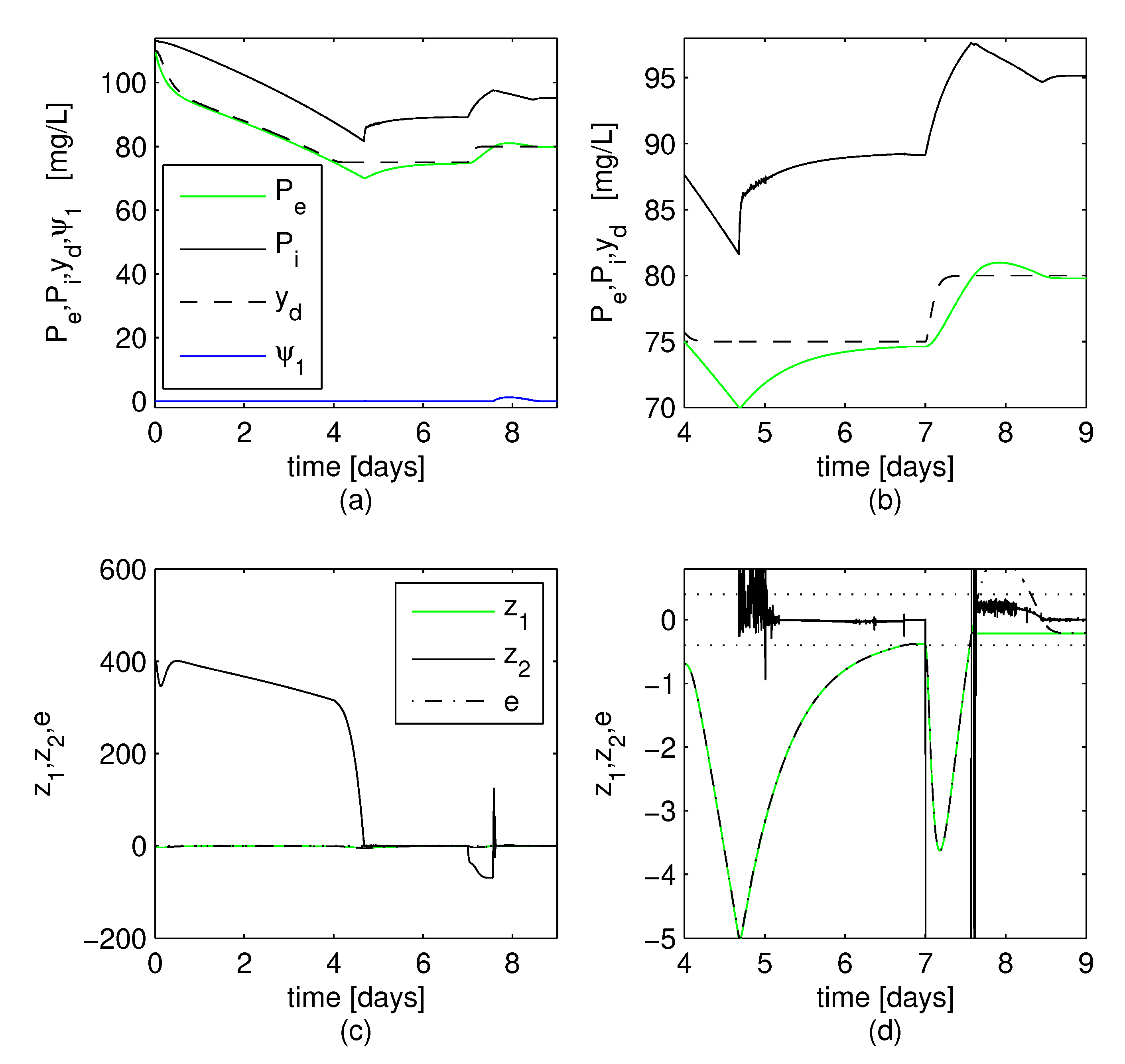
Consider the aeroponic system described in Appendix A whose model is given by Equations (1)–(3), with input constraint (4), Assumptions 1–5, and control goal and desired output y d stated in Section 2.2 and Section 2.3. The control law, the update laws, the auxiliary system, and their parameters and signals are stated in Remark 5. At what follows, the values of x 1 , x 2 and x 3 are generated through the model (1) to (3) with specific parameter values. These values of x 1 , x 2 and x 3 are used by the controller, but the model parameters and upper or lower bounds are not.
The input saturation values are u m i n = 0 and
u m a x = 350 L / day for t 7 days 10.944 L / day otherwise .
The input value Q a d = 0 is used until x 1 reaches the value 70 mg/L, so that the controller is started at t = 4 days. The parameters of the reference model (5) are chosen as a m 1 = 40 and
W r e f = 75 mg / L for t 7 days 80 mg / L otherwise ,
whereas the desired width of the convergence region is chosen to be C b = 0.4 . The user-defined parameters of the control law, update laws and auxiliary system are chosen as
k 1 = 8 for t 7 days 2 otherwise ,
k 2 = 0.005 , k ψ 1 = 20 > 1 / 2 , k ψ 2 = 20 > 1 / 2 , γ 1 , 1 = 8 × 10 4 , γ 1 , 2 = 0.008 , γ r x 1 = 4 × 10 7 , γ 3 = 0.004 , γ i l b = 4 × 10 7 , γ u b = 4 × 10 9 , γ 4 = 4 × 10 4 .
We consider the measurement noise for x 3 in the control gain b, such that b satisfies the first condition of assumption 2.5, with
b m = P a d x 2 x 3 m , b δ = x 3 m x 3
Due to the controller starting at t = 4 days and the change of W r e f at t = 7 days, the system behavior is separated in the time intervals [ 4 7 ) and [ 7 ) days. For t [ 4 7 ) days:
  • all the closed loop signals are bounded (see Figure 1, Figure 2 and Figure 3).
  • the signal z 1 is near Ω z 1 at initial time ( z 1 t o 0.7 ) , it enters Ω z 1 at 6.72 days and it remains inside until t = 7 days (Figure 1d).
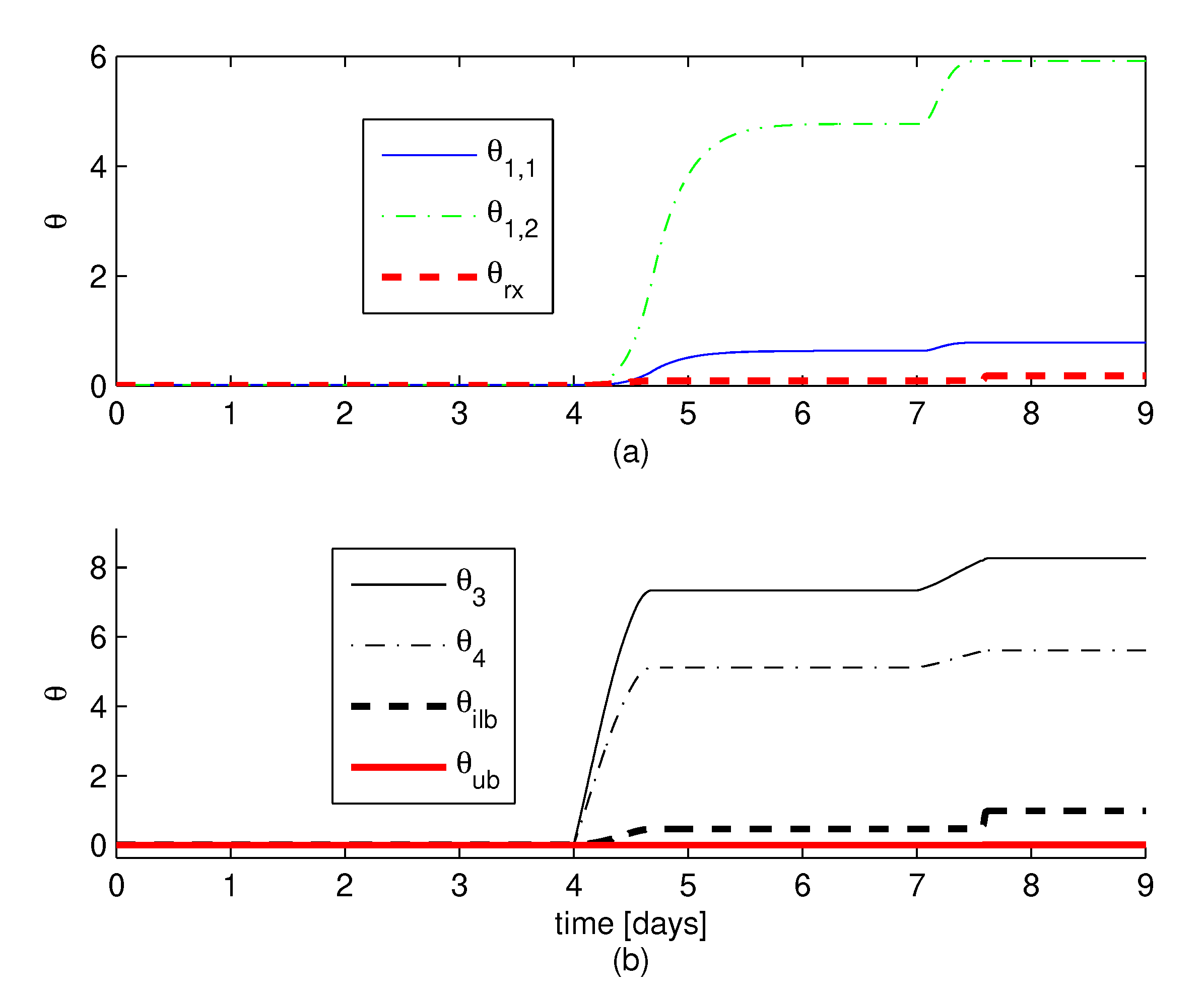
  • the updated parameters remain bounded, and its change is not excessive; θ ^ 1 , 1 , θ ^ 1 , 2 change when z 1 Ω z 1 , and remain constant otherwise (Figure 3).
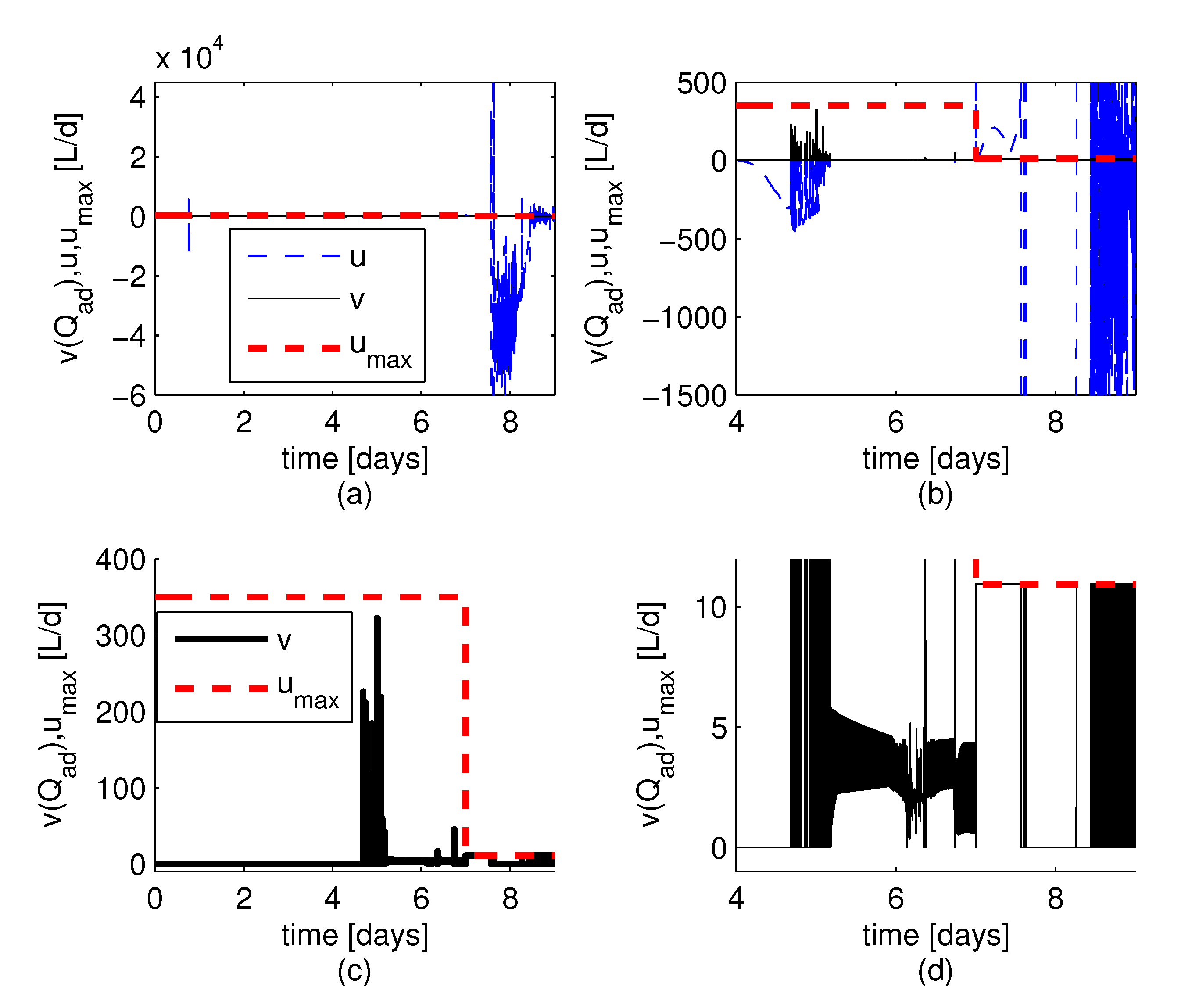
  • input signal v: for t [ 4 5.09 ] [ 6.52 6.6 ] days it exhibits reiterated saturation at its lower bound, with only one moment of saturation at its upper bound (at t = 4.89 days approx); during other moments it exhibits changing behavior (Figure 2c,d).
For t 7 days:
  • all the closed loop signals are bounded (see Figure 1, Figure 2 and Figure 3).
  • the signal z 1 is inside Ω z 1 at t = 7 days ( z 1 t o 0.39 ) , it leaves, it enters Ω z 1 at 7.55 days approx. and it remains inside afterwards (Figure 1d).
  • the updated parameters remain bounded, θ ^ 1 , 1 , θ ^ 1 , 2 are constant when z 1 Ω z 1 , and the other updated parameters are constant when z 2 Ω z 2 (Figure 3).
  • input signal v: for t [ 7.0 7.57 ] days, it remains saturated at its upper bound; for t ( 7.57 8.44 ] days, it exhibits saturation at its lower bound with some few saturation at its upper bounds; for t > 8.44 days, it exhibits reiterated saturation at both its upper and lower bounds (Figure 2c,d).

5. Conclusions

In this paper, an adaptive backstepping controller was developed for a second order plant model subject to unknown model parameters, unknown reaction rate, unknown varying control gain, and input saturation. The controller provides important contributions to adaptive control design for second-order models with input saturation:
  • It tackles the combined effect of constrained control input and unknown varying control gain with unknown bounds. To this end, a new auxiliary system is proposed.
  • The modified tracking error asymptotically converges to a compact set whose width is user-defined and it does not depend on bounds of either external disturbances, model terms or parameters. Recall that in common robust backstepping designs, the tracking error converges to a compact set whose width depends on such kind of bounds, so that these bounds are required in order to obtain the expected width.
Other important features of the controller and closed loop system are
  • the model coefficients, and upper and lower bounds of model terms are not required to be known, except a 1 ;
  • the exact value of the reaction rate term r x 1 is not required to be known;
  • the control gain b is varying and unknown, although it can be expressed as b = b δ b x , where b x is known and b δ is unknown;
  • discontinuous functions are not used in the control law, update laws and auxiliary system; instead, saturation type functions are used; and
  • the boundedness of the updated parameters is ensured in the presence of input saturation, so that excessive parameter increase is avoided.
Significant improvements were made to the control design in order to tackle the unknown varying nature of the control gain b and the input saturation. Dead zone radially unbounded functions were used. As the gain b appears in the b Δ term, the design of the auxiliary system must be modified.
The developed controller design can be applied to other second order nonlinear systems as the mathematical manipulations are provided.

Author Contributions

Conceptualization, A.R.; methodology, A.R.; validation, F.E.H. and J.E.C.-B.; formal analysis, A.R., F.E.H., and J.E.C.-B.; investigation, A.R.; writing—original draft preparation, A.R.; writing–review and editing, A.R., F.E.H., and J.E.C.-B.; visualization, F.E.H. and J.E.C.-B. All authors have read and agreed to the published version of the manuscript.

Funding

The work of A. Rincón was supported by Universidad Católica de Manizales. The work of F.E. Hoyos and J.E. Candelo-Becerra was supported by Universidad Nacional de Colombia—Sede Medellín.

Conflicts of Interest

The authors declare no conflict of interest.

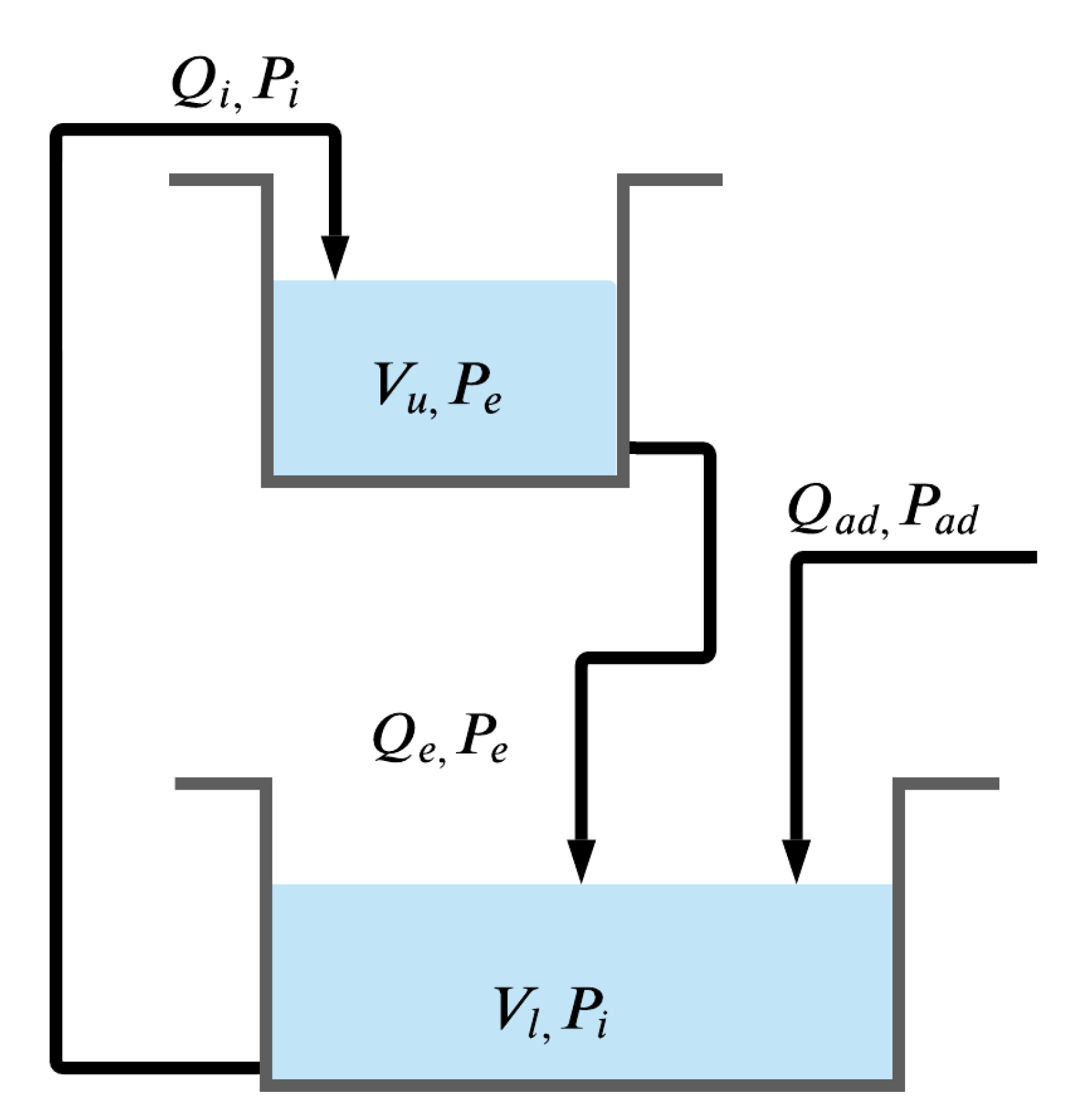
Appendix A. Hydroponic System and Formulation of the Mass Balance Model

The hydroponic system of the work in [28] comprises three vertical cultivation beds with grown tomatoes, a nutrient solution tank (mixing tank), a closed nutrient solution circulation system, and a lighting system. An electric pump drives a fraction of the nutrient solution from the mixing tank to the cultivation beds, and the drainage solution is conveyed back to the mixing tank. The mixing tank is eventually replenished with new nutrient solution in order to maintain a high EC, near 1.5 mS/cm. The nutrient solution in the mixing tank exhibits decrease of electrical conductivity (EC) and concentration of major ions during time periods with no addition of fresh nutrient solution, whereas there is an increase of EC during addition of nutrient solution [28].
We consider the control of concentration of some major ion in the cultivation bed, by manipulation of the flow of fresh nutrient solution to the mixing tank ( Q a d ) , considering constant flows Q i and Q e . To this end, the mass balance model is developed for the concentration of some general nutrient ion, but in the simulation example the N O 3 N ion is considered, because its behavior is quite similar to that of the electrical conductivity (EC). We consider the mixing tank, the cultivation beds with plants, the flow of addition of fresh nutrient solution to the mixing tank, and the flows of nutrient solution between the mixing tank and the cultivation beds. We assume that the system can be represented by two linked continuous stirred tank reactors (CSTR), see Figure A1:
  • The upper CSTR corresponds to the nutrient solution in the cultivation beds. The nutrient concentration is denoted as P e , the water volume is denoted as V u , the rate of nutrient removal is denoted as r x 1 , and the evapotranspiration rate is denoted as Q E T . Nutrient removal occurs via sorption and plant uptake. We assume that the water volume V u is constant.
  • The lower CSTR corresponds to the nutrient solution in the mixing tank. The nutrient concentration is denoted as P i and the water volume is denoted as V l . The nutrient solution mixes with the incoming flow, which is in turn the flow leaving the upper CSTR. We assume that V l is varying because of water evaporation losses and varying nature of flow Q a d .
Figure A1. Schematic diagram of the CSTR-based model for the hydroponic system.
Applsci 11 00251 g0a1
In addition, Q i is the flowrate that leaves the lower CSTR and enters the upper CSTR, and Q e is the flowrate that leaves the upper CSTR and enters the lower CSTR. The outflow ( Q e ) is lower than the inflow ( Q i ) , due to evapotranspiration and constant nature of volume V u . We assume that flows Q i and Q e are constant. The development of the mass balance model gives as result the model (1) to (3).
This model with the reaction rate expression
r x 1 = μ m x P e K + P e + μ o
was fitted to the experimental data of N O 3 N shown in [28], time interval 20–33 days, which corresponds to stage II (adaptation). This was performed by minimization of the squares of the errors between experimental and simulated values of N O 3 N ( P i ) [29]. The obtained model parameters are a 1 = 3.55 days 1 , a 2 = 3.485 days 1 , a 3 = 3.254 L/day, a 4 = 0.1066 L/day, P a d = 110 mg/L, μ m x = 1051.6 mg/(Ld), K = 1509.8 mg/L, and μ o = 6.903 mg/(Ld).

References

  1. Schaum, A.; Alvarez, J.; Garcia-Sandoval, J.P.; Gonzalez-Alvarez, V.M. On the dynamics and control of a class of continuous digesters. J. Process Control 2015, 34, 82–96. [Google Scholar] [CrossRef]
  2. Battista, H.D.; Jamilis, M.; Garelli, F. Global stabilisation of continuous bioreactors: Tools for analysis and design of feeding laws. Automatica 2018, 89, 340–348. [Google Scholar] [CrossRef]
  3. Battista, H.D.; Picó, J.; Picó-Marco, E. Nonlinear PI control of fed-batch processes for growth rate regulation. J. Process Control 2012, 22, 789–797. [Google Scholar] [CrossRef]
  4. Dalal, P.; Roy, S.; Chopda, V.; Gomes, J.; Rathore, A.S. Comparison and implementation of different control strategies for improving production of rHSA using Pichia pastoris. J. Biotechnol. 2019, 290, 33–43. [Google Scholar]
  5. Lara-Cisneros, G.; Femat, R.; Dochain, D. An extremum seeking approach via variable-structure control for fed-batch bioreactors with uncertain growth rate. J. Process Control 2014, 24, 663–671. [Google Scholar] [CrossRef]
  6. Nuñez, S.; Garelli, F.; Battista, H.D. Closed-loop growth-rate regulation in fed-batch dual-substrate processes with additive kinetics based on biomass concentration measurement. J. Process Control 2016, 44, 14–22. [Google Scholar] [CrossRef]
  7. Petre, E.; Selisteanu, D.; Sendrescu, D. Adaptive and robust-adaptive control strategies for anaerobic wastewater treatment bioprocesses. Chem. Eng. J. 2013, 217, 363–378. [Google Scholar] [CrossRef]
  8. Bastin, G.; Dochain, D. On-Line Estimation and Adaptive Control of Bioreactors; Elsevier: Amsterdam, The Netherlands, 1990. [Google Scholar]
  9. Méndez-Acosta, H.O.; Campos-Delgado, D.U.; Femat, R.; González-Alvarez, V. A robust feedforward/feedback control for an anaerobic digester. Comput. Chem. Eng. 2005, 29, 1613–1623. [Google Scholar] [CrossRef]
  10. Polycarpou, M.; Farrell, J.; Sharma, M. On-line approximation control of uncertain nonlinear systems: Issues with control input saturation. In Proceedings of the American Control Conference, Denver, CO, USA, 4–6 June 2003; pp. 543–548. [Google Scholar]
  11. Gao, S.; Ning, B.; Dong, H. Fuzzy dynamic surface control for uncertain nonlinear systems under input saturation via truncated adaptation approach. Fuzzy Set. Syst. 2016, 290, 100–117. [Google Scholar] [CrossRef]
  12. Min, H.; Xu, S.; Ma, Q.; Zhang, B.; Zhang, Z. Composite-observer-based output-feedback control for nonlinear time-delay systems with input saturation and its application. IEEE Trans. Ind. Electron. 2018, 65, 5856–5863. [Google Scholar] [CrossRef]
  13. Lin, D.; Wang, X.; Yao, Y. Fuzzy neural adaptive tracking control of unknown chaotic systems with input saturation. Nonlinear Dynam. 2012, 67, 2889–2897. [Google Scholar] [CrossRef]
  14. Askari, M.R.; Shahrokhi, M.; Talkhoncheh, M.K. Observer-based adaptive fuzzy controller for nonlinear systems with unknown control directions and input saturation. Fuzzy Set. Syst. 2017, 314, 24–45. [Google Scholar] [CrossRef]
  15. Nassira, Z.; Mohamed, C.; Essounbouli, N. Adaptive neural-network output feedback control design for uncertain CSTR system with input saturation. In Proceedings of the 2018 International Conference on Electrical Sciences and Technologies, CISTEM, Algiers, Algeria, 29–31 October 2019. [Google Scholar]
  16. Astrom, K.J.; Wittenmark, B. Adaptive Control; Addison-Wesley Publising Company: Reading, MA, USA, 1995. [Google Scholar]
  17. Slotine, J.; Li, W. Applied Nonlinear Control; Prentice-Hall Inc.: Englewood Cliffs, NJ, USA, 1991. [Google Scholar]
  18. Polycarpou, M.M.; Ioannou, P.A. On the existence and uniqueness of solutions in adaptive control systems. IEEE Trans. Automat. Control 1993, 38, 474–479. [Google Scholar] [CrossRef]
  19. Polycarpou, M.M.; Ioannou, P.A. A robust adaptive nonlinear control design. Automatica 1996, 32, 423–427. [Google Scholar] [CrossRef]
  20. Rincon, A.; Piarpuzán, D.; Angulo, F. A new adaptive controller for bio-reactors with unknown kinetics and biomass concentration: Guarantees for the boundedness and convergence properties. Math. Comput. Simulat. 2015, 112, 1–13. [Google Scholar] [CrossRef]
  21. Zhou, J.; Zhang, C.; Wen, C. Robust adaptive output control of uncertain nonlinear plants with unknown backlash nonlinearity. IEEE T. Automat. Control 2007, 52, 503–509. [Google Scholar] [CrossRef]
  22. Koo, K. Stable adaptive fuzzy controller with time-varying dead-zone. Fuzzy Set. Syst. 2001, 121, 161–168. [Google Scholar] [CrossRef]
  23. Wang, X.; Su, C.; Hong, H. Robust adaptive control of a class of nonlinear systems with unknown dead-zone. Automatica 2004, 40, 407–413. [Google Scholar] [CrossRef]
  24. Su, C.; Feng, Y.; Hong, H.; Chen, X. Adaptive control of system involving complex hysteretic nonlinearities: A generalised Prandtl–Ishlinskii modelling approach. Int. J. Control 2009, 82, 1786–1793. [Google Scholar] [CrossRef]
  25. Wang, Q.; Su, C. Robust adaptive control of a class of nonlinear systems including actuator hysteresis with Prandtl–Ishlinskii presentations. Automatica 2006, 42, 859–867. [Google Scholar] [CrossRef]
  26. Ranjbar, E.; Yaghubi, M.; Suratgar, A.A. Robust adaptive sliding mode control of a MEMS tunable capacitor based on dead-zone method. Automatika 2020, 61, 587–601. [Google Scholar] [CrossRef]
  27. Ioannou, P.; Sun, J. Robust Adaptive Control; Prentice-Hall PTR: Upper Saddle River, NJ, USA, 1996. [Google Scholar]
  28. Lee, J.Y.; Rahman, A.; Azam, H.; Kim, H.S.; Kwon, M.J. Characterizing nutrient uptake kinetics for efficient crop production during Solanum lycopersicum var. cerasiforme Alef. growth in a closed indoor hydroponic system. PLoS ONE 2017, 12, e0177041. [Google Scholar] [CrossRef] [PubMed]
  29. Mutolsky, H.; Christopoulos, A. Fitting Models to Biological Data Using Linear and Nonlinear Regression; GraphPad Software: San Diego, CA, USA, 2003. [Google Scholar]
Figure 1. Simulation results for the system signals under the formulated controller. (a) Time course of the states P e , P i , desired output y d , and auxiliary signal ψ 1 . (b) Detail of the time course of P e , P i , and y d . (c) Time course of the modified tracking error z 1 , signal z 2 and tracking error e. (d) Detail of the signals z 1 , z 2 , and e; the horizontal dotted lines represent C b and C b .
Applsci 11 00251 g001
Figure 2. Simulation results for the system signals under the formulated controller. (a) Time course of the non-saturated input u and the saturated input v. (b) Detail of the time course of signals u and v. (c) Time course of the saturated input v. (d) Detail of the signal v.
Applsci 11 00251 g002
Figure 3. Simulation results for the system signals under the formulated controller. (a) Time course of the updated parameters θ ^ 1 , 1 , θ ^ 1 , 2 , θ ^ r x . (b) Time course of the updated parameters θ ^ 3 , θ ^ 4 , θ ^ i l b , θ ^ u b .
Applsci 11 00251 g003
Publisher’s Note: MDPI stays neutral with regard to jurisdictional claims in published maps and institutional affiliations.

