Predicting the Risk of Chronic Kidney Disease (CKD) Using Machine Learning Algorithm


Abstract
1. Introduction
2. Materials and Methods
2.1. Dataset
2.2. Regression Methods
2.2.1. Random Forest
2.2.2. XGBoost
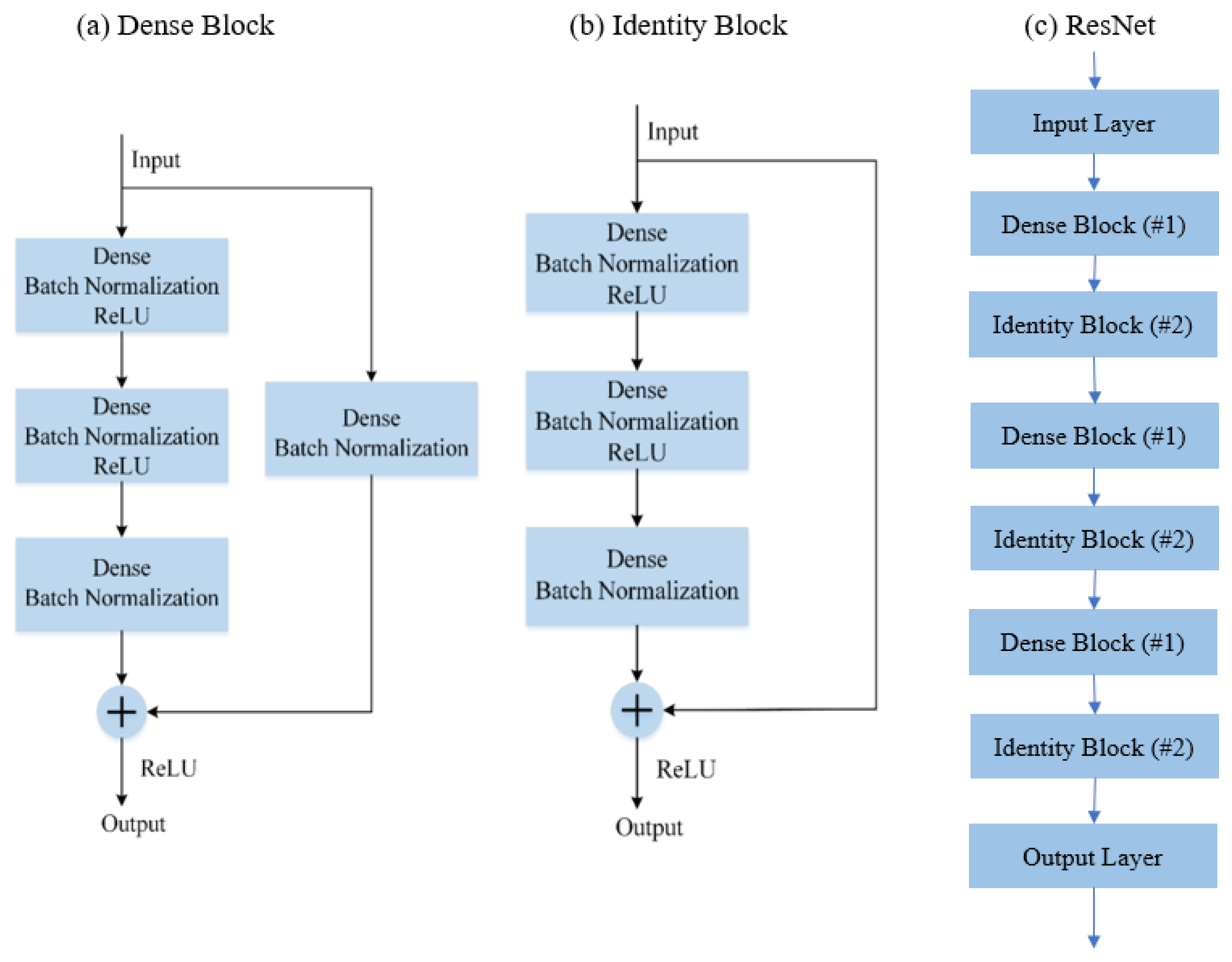
2.2.3. RestNet
3. Proposed Methodology
3.1. Preprocessing Method
- (i)
- Some samples have missing values on some attributes. As we already have a large data, 8654 samples with one or more missing attributes are removed.
- (ii)
- There are some data with very large values of creatinine. Those samples are from patients at a late stage of renal failure. These subjects are not targets of this work, and therefore such data are classed as outlier data as far as training our target model is concerned. We removed 1234 samples with a value of creatinine higher than 2.5 mL/min.
- (iii)
- In the original data, the attribute of Sex and SMK_STATE are not suitable for numerical coding. We changed them into one-hot coding format. We remove original variables and replace them with new binary variables where 0 is the value when the category is false and 1 when it is true. For example, sex is replaced by Male and Female, two attributes. For a Male subject, Male attribute is assigned a value “1” and female as “0”.
3.2. Undersampling for Data Balancing
3.2.1. Extremely Unbalanced Data
3.2.2. Details about Undersampling
3.3. Cost-Sensitive MSE Loss Function
- (a)
- Calculate the range of target variable (Range) and minimum value of target variable (Min).
- (b)
- Split the data into 10 subsets depending on Range. For example, samples with target variable larger than (0.2 × Range + Min) and smaller than (0.3 × Range + Min) belong to subset_3.
- (c)
- After the first training epoch, calculate the mean error of each subset, which is named the .
- (d)
- Calculate the mean value of for 10 subsets, which is the .
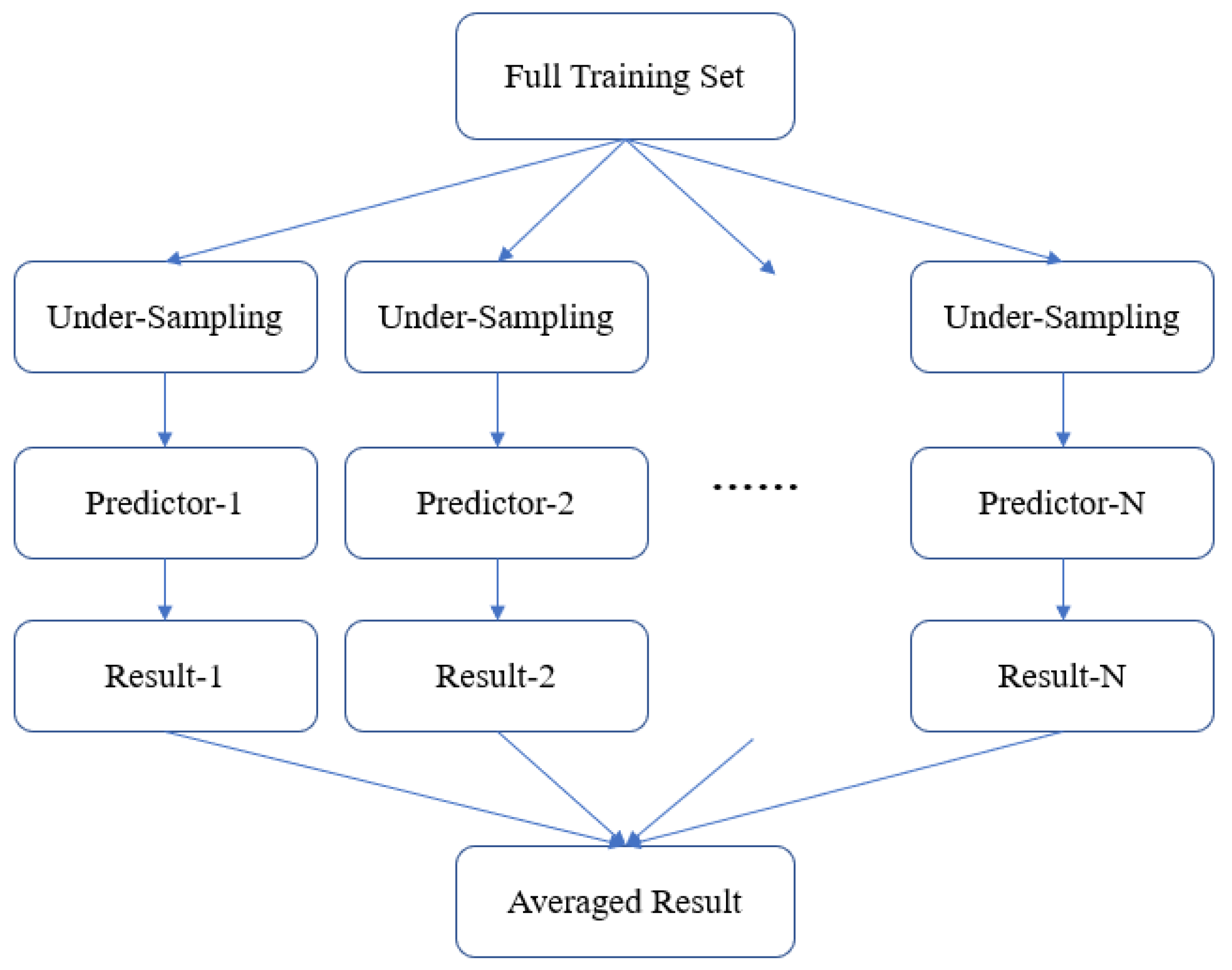
3.4. Model Ensemble Strategy
4. Experiments and Results
4.1. Evaluation Method
4.2. Experiments with Different Undersampling Strategies
4.3. Experiments with Different Regression Algorithms
4.4. Experiments with Cost-Sensitive Loss Function
4.5. Experiments with Model Ensemble
4.6. Prediction the Risk of CKD
5. Conclusions and Future Work
Author Contributions
Funding
Data Availability Statement
Conflicts of Interest
References
- Stevens, P.E.; Levin, A. Evaluation and management of chronic kidney disease: Synopsis of the kidney disease: Improving global outcomes 2012 clinical practice guideline. Ann. Intern. Med. 2013, 158, 825–830. [Google Scholar] [CrossRef] [PubMed]
- Bikbov, B.; Perico, N.; Remuzzi, G. Disparities in chronic kidney disease prevalence among males and females in 195 countries: Analysis of the Global Burden of Disease 2016 Study. Nephron 2018, 139, 313–318. [Google Scholar] [CrossRef] [PubMed]
- Couser, W.G.; Remuzzi, G.; Mendis, S.; Tonelli, M. The contribution of chronic kidney disease to the global burden of major noncommunicable diseases. Kidney Int. 2011, 80, 1258–1270. [Google Scholar] [CrossRef] [PubMed]
- National Institute of Diabetes and Digestive and Kidney Diseases. Chronic Kidney Disease Tests and Diagnosis; National Institute of Diabetes and Digestive and Kidney Diseases: Bethesda, MD, USA, 2016.
- Yarnoff, B.O.; Hoerger, T.J.; Simpson, S.K.; Leib, A.; Burrows, N.R.; Shrestha, S.S.; Pavkov, M.E. The cost-effectiveness of using chronic kidney disease risk scores to screen for early-stage chronic kidney disease. BMC Nephrol. 2017, 18, 85. [Google Scholar] [CrossRef] [PubMed]
- Kuo, C.C.; Chang, C.M.; Liu, K.T.; Lin, W.K.; Chiang, H.Y.; Chung, C.W.; Ho, M.R.; Sun, P.R.; Yang, R.L.; Chen, K.T. Automation of the kidney function prediction and classification through ultrasound-based kidney imaging using deep learning. NPJ Digit. Med. 2019, 2, 1–9. [Google Scholar] [CrossRef] [PubMed]
- Basak, S.; Alam, M.M.; Rakshit, A.; Al Marouf, A.; Majumder, A. Predicting and Staging Chronic Kidney Disease of Diabetes (Type-2) Patient Using Machine Learning Algorithms. Int. J. Innov. Technol. Explor. Eng. 2019, 8. [Google Scholar] [CrossRef]
- Kumar, M. Prediction of chronic kidney disease using random forest machine learning algorithm. Int. J. Comput. Sci. Mob. Comput. 2016, 5, 24–33. [Google Scholar]
- Rady, E.H.A.; Anwar, A.S. Prediction of kidney disease stages using data mining algorithms. Inform. Med. Unlocked 2019, 15, 100178. [Google Scholar] [CrossRef]
- Chimwayi, K.B.; Haris, N.; Caytiles, R.D.; Iyengar, N.C.S. Risk Level Prediction of Chronic Kidney Disease Using Neuro-Fuzzy and Hierarchical Clustering Algorithm (s). Int. J. Multimedia Ubiq. Eng. 2017, 12, 23–36. [Google Scholar] [CrossRef]
- Almansour, N.A.; Syed, H.F.; Khayat, N.R.; Altheeb, R.K.; Juri, R.E.; Alhiyafi, J.; Alrashed, S.; Olatunji, S.O. Neural network and support vector machine for the prediction of chronic kidney disease: A comparative study. Comput. Biol. Med. 2019, 109, 101–111. [Google Scholar] [CrossRef]
- Salekin, A.; Stankovic, J. Detection of chronic kidney disease and selecting important predictive attributes. In Proceedings of the 2016 IEEE International Conference on Healthcare Informatics (ICHI), Chicago, IL, USA, 4–7 October 2016. [Google Scholar]
- Almasoud, M.; Ward, T.E. Detection of chronic kidney disease using machine learning algorithms with least number of predictors. Int. J. Soft Comput. Its Appl. 2019, 10. [Google Scholar] [CrossRef]
- Rubini, L.; Jerlin. Department of Computer Science and Engineering, Algappa University: TamilNadu. 2015. Available online: http://archive.ics.uci.edu/ml/datasets/Chronic_Kidney_Disease (accessed on 8 June 2020).
- Liaw, A.; Wiener, M. Classification and regression by randomForest. R News 2002, 2, 18–22. [Google Scholar]
- Chen, T.; Guestrin, C. Xgboost: A scalable tree boosting system. In Proceedings of the 22nd ACM Sigkdd International Conference on Knowledge Discovery and Data Mining, San Francisco, CA, USA, 13–17 August 2016; pp. 785–794. [Google Scholar]
- Chen, D.; Hu, F.; Nian, G.; Yang, T. Deep Residual Learning for Nonlinear Regression. Entropy 2020, 22, 193. [Google Scholar] [CrossRef] [PubMed]
- Friedman, J.H. Greedy function approximation: A gradient boosting machine. Ann. Stat. 2001, 1189–1232. [Google Scholar] [CrossRef]
- Buda, M.; Maki, A.; Mazurowski, M.A. A systematic study of the class imbalance problem in convolutional neural networks. Neural Netw. 2017, 106, 249–259. [Google Scholar] [CrossRef] [PubMed]


| Ser | Variable | Type | Class | Description |
|---|---|---|---|---|
| 1 | Sex | Categorical | Predictor | |
| 2 | Age | Numerical | Predictor | |
| 3 | Waist | Numerical | Predictor | |
| 4 | Listen_left | Categorical | Predictor | hearing impairment or not |
| 5 | Listen_right | Categorical | Predictor | hearing impairment or not |
| 6 | Vision_left | Numerical | Predictor | |
| 7 | Vision_right | Numerical | Predictor | |
| 8 | BP_HIGH | Numerical | Predictor | systolic pressure |
| 9 | BP_LWST | Numerical | Predictor | diastolic pressure |
| 10 | BLDS | Numerical | Predictor | fasting blood sugar |
| 11 | TOT_CHOLE | Numerical | Predictor | total cholesterol |
| 12 | TRIGLYCERIDE | Numerical | Predictor | triglycerides |
| 13 | HDL_CHOLE | Numerical | Predictor | high-density lipoprotein cholesterol |
| 14 | LDL_CHOLE | Numerical | Predictor | low-density lipoprotein cholesterol |
| 15 | HMG | Numerical | Predictor | hemoglobin |
| 16 | OLIG_PROTE_CD | Categorical | Predictor | the level of urine protein |
| 17 | SGOT_AST | Numerical | Predictor | aspartate amino-transferase |
| 18 | SGPT_ALT | Numerical | Predictor | alanine amino-transferase |
| 19 | GAMMA_GTP | Numerical | Predictor | gamma glutamyl transpeptidas |
| 20 | SMK_STATE | Categorical | Predictor | smoking status |
| 21 | DRINK_OR_NOT | Categorical | Predictor | drink habit |
| 22 | MOUTH_CHECK | Categorical | Predictor | decayed teeth or not |
| 23 | BMI | Numerical | Predictor | calculated using height and weight |
| 24 | CREATININE | Numerical | Target_1 | serum creatinine |
| 25 | GFR | Numerical | calculated using Equation (1) | |
| 26 | Stage | Categorical | determined from GFR | |
| 27 | CKD | Binary | Target_2 | GFR < stage 2 (class 1) or not (class 0, normal) |
| Stage | GFR (mL/min) | Description |
|---|---|---|
| Stage 1 | 90 or higher | normal |
| Stage 2 | 89 to 60 | mild loss |
| Stage 3a | 59 to 45 | mild to moderate |
| Stage 3b | 44 to 30 | moderate to severe |
| Stage 4 | 29 to 15 | severe |
| Stage 5 | less than 15 | failure |
| Creatinine | Original | Sampling-1 | Sampling-2 | Sampling-3 | Sampling-4 | Sampling-5 | Sampling-6 |
|---|---|---|---|---|---|---|---|
| 0.1 | 395 | 395 | 395 | 395 | 395 | 395 | 395 |
| 0.2 | 93 | 93 | 93 | 93 | 93 | 93 | 93 |
| 0.3 | 549 | 549 | 549 | 549 | 549 | 549 | 549 |
| 0.4 | 5503 | 5503 | 5503 | 5000 | 2500 | 1200 | 600 |
| 0.5 | 35,395 | 20,000 | 10,000 | 5000 | 2500 | 1200 | 600 |
| 0.6 | 99,185 | 20,000 | 10,000 | 5000 | 2500 | 1200 | 600 |
| 0.7 | 149,238 | 20,000 | 10,000 | 5000 | 2500 | 1200 | 600 |
| 0.8 | 177,224 | 20,000 | 10,000 | 5000 | 2500 | 1200 | 600 |
| 0.9 | 164,153 | 20,000 | 10,000 | 5000 | 2500 | 1200 | 600 |
| 1.0 | 127,881 | 20,000 | 10,000 | 5000 | 2500 | 1200 | 600 |
| 1.1 | 78,432 | 20,000 | 10,000 | 5000 | 2500 | 1200 | 600 |
| 1.2 | 37,180 | 20,000 | 10,000 | 5000 | 2500 | 1200 | 600 |
| 1.3 | 13,873 | 13,873 | 10,000 | 5000 | 2500 | 1200 | 600 |
| 1.4 | 5216 | 5216 | 5216 | 5000 | 2500 | 1200 | 600 |
| 1.5 | 2224 | 2224 | 2224 | 2224 | 2224 | 1200 | 600 |
| 1.6 | 1160 | 1160 | 1160 | 1160 | 1160 | 1160 | 600 |
| 1.7 | 687 | 687 | 687 | 687 | 687 | 687 | 600 |
| 1.8 | 523 | 523 | 523 | 523 | 523 | 523 | 523 |
| 1.9 | 309 | 309 | 309 | 309 | 309 | 309 | 309 |
| 2.0 | 235 | 235 | 235 | 235 | 235 | 235 | 235 |
| 2.1 | 144 | 144 | 144 | 144 | 144 | 144 | 144 |
| 2.2 | 137 | 137 | 137 | 137 | 137 | 137 | 137 |
| 2.3 | 92 | 92 | 92 | 92 | 92 | 92 | 92 |
| 2.4 | 96 | 96 | 96 | 96 | 96 | 96 | 96 |
| 2.5 | 76 | 76 | 76 | 76 | 76 | 76 | 76 |
| Sum | 900,000 | 191,312 | 107,439 | 61,757 | 34,220 | 18,896 | 11,049 |
| Test Set | Original | Sampling-1 | Sampling-2 | Sampling-3 | Sampling-4 | Sampling-5 | Sampling-6 |
|---|---|---|---|---|---|---|---|
| 1 | 0.2507 | 0.4586 | 0.5065 | 0.5389 | 0.5581 | 0.5667 | 0.5532 |
| 2 | 0.2488 | 0.4540 | 0.5005 | 0.5389 | 0.5562 | 0.5622 | 0.5473 |
| 3 | 0.2507 | 0.4521 | 0.4967 | 0.5309 | 0.5455 | 0.5543 | 0.5384 |
| 4 | 0.2484 | 0.4538 | 0.5017 | 0.5341 | 0.5574 | 0.5633 | 0.5482 |
| 5 | 0.2498 | 0.4537 | 0.5026 | 0.5348 | 0.5526 | 0.5604 | 0.5426 |
| 6 | 0.2468 | 0.4507 | 0.4977 | 0.5313 | 0.5453 | 0.5585 | 0.5407 |
| 7 | 0.2447 | 0.4484 | 0.4997 | 0.5358 | 0.5545 | 0.5644 | 0.5492 |
| 8 | 0.2461 | 0.4499 | 0.4948 | 0.5328 | 0.5471 | 0.5544 | 0.5359 |
| 9 | 0.2449 | 0.4494 | 0.4997 | 0.5361 | 0.5561 | 0.5649 | 0.5523 |
| 10 | 0.2423 | 0.4472 | 0.4973 | 0.5326 | 0.5499 | 0.5618 | 0.5499 |
| Average | 0.2473 | 0.4518 | 0.4997 | 0.5346 | 0.5523 | 0.5591 | 0.5458 |
| Test Set | Random Forest | XGBoost | ResNet |
|---|---|---|---|
| 1 | 0.5392 | 0.5581 | 0.5322 |
| 2 | 0.5369 | 0.5562 | 0.5266 |
| 3 | 0.5289 | 0.5455 | 0.5265 |
| 4 | 0.5362 | 0.5574 | 0.5338 |
| 5 | 0.5337 | 0.5526 | 0.5357 |
| 6 | 0.5289 | 0.5453 | 0.5254 |
| 7 | 0.5387 | 0.5545 | 0.5353 |
| 8 | 0.5267 | 0.5417 | 0.5238 |
| 9 | 0.5389 | 0.5561 | 0.5288 |
| 10 | 0.5353 | 0.5499 | 0.5289 |
| Average | 0.5343 | 0.5523 | 0.5297 |
| Variable | Decrease in Gini Index |
|---|---|
| Sex | 0.49 |
| Age | 0.11 |
| HMG | 0.10 |
| OLIG_PROTE_CD | 0.08 |
| Waist | 0.04 |
| SMOKE_STATE | 0.04 |
| Error Using Data Subset | Number of Data in the Subset | Without Cost- Sensitive Loss | Error Comparison | With Cost- Sensitive Loss |
|---|---|---|---|---|
| 1 | 840 | 0.6125 | > | 0.6036 |
| 2 | 2000 | 0.2065 | > | 0.1974 |
| 3 | 3000 | 0.1693 | < | 0.1799 |
| 4 | 2000 | 0.1952 | < | 0.1972 |
| 5 | 3000 | 0.1336 | < | 0.1544 |
| 6 | 2000 | 0.2309 | < | 0.2422 |
| 7 | 1710 | 0.2896 | > | 0.2831 |
| 8 | 870 | 0.4746 | > | 0.4081 |
| 9 | 220 | 0.5332 | > | 0.4560 |
| 10 | 280 | 0.8235 | > | 0.6965 |
| Predictor | P1 | P2 | P3 | P4 | P5 | P6 | P7 | P8 | Average | |
|---|---|---|---|---|---|---|---|---|---|---|
| Test Set | ||||||||||
| 1 | 0.5562 | 0.5574 | 0.5576 | 0.5569 | 0.5591 | 0.5568 | 0.5624 | 0.5599 | 0.5583 | |
| 2 | 0.5537 | 0.5483 | 0.5562 | 0.5551 | 0.5559 | 0.5519 | 0.5542 | 0.5538 | 0.5536 | |
| 3 | 0.5449 | 0.5421 | 0.5516 | 0.5432 | 0.5476 | 0.5433 | 0.5512 | 0.5483 | 0.5465 | |
| 4 | 0.5617 | 0.5605 | 0.5656 | 0.5625 | 0.5589 | 0.5509 | 0.5625 | 0.5614 | 0.5605 | |
| 5 | 0.5498 | 0.5505 | 0.5530 | 0.5502 | 0.5496 | 0.5507 | 0.5526 | 0.5522 | 0.5511 | |
| 6 | 0.5498 | 0.5474 | 0.5503 | 0.5499 | 0.5508 | 0.5483 | 0.5531 | 0.5503 | 0.5500 | |
| 7 | 0.5635 | 0.5650 | 0.5690 | 0.5664 | 0.5707 | 0.5676 | 0.5708 | 0.5680 | 0.5676 | |
| 8 | 0.5520 | 0.5511 | 0.5527 | 0.5503 | 0.5502 | 0.5528 | 0.5560 | 0.5539 | 0.5524 | |
| 9 | 0.5592 | 0.5512 | 0.5585 | 0.5571 | 0.5595 | 0.5533 | 0.5585 | 0.5573 | 0.5568 | |
| 10 | 0.5497 | 0.5458 | 0.5491 | 0.5495 | 0.5483 | 0.5473 | 0.5499 | 0.5459 | 0.5482 | |
| Average | 0.5541 | 0.5519 | 0.5564 | 0.5541 | 0.5551 | 0.5533 | 0.5571 | 0.5551 | 0.5546 | |
| Test Set | 1P | 2Ps | 3Ps | 4Ps | 5Ps | 6Ps | 7Ps | 8Ps |
|---|---|---|---|---|---|---|---|---|
| 1 | 0.5562 | 0.5596 | 0.5605 | 0.5608 | 0.5615 | 0.5615 | 0.5623 | 0.5626 |
| 2 | 0.5537 | 0.5538 | 0.5562 | 0.5571 | 0.5579 | 0.5577 | 0.5580 | 0.5581 |
| 3 | 0.5449 | 0.5462 | 0.5497 | 0.5492 | 0.5499 | 0.5496 | 0.5506 | 0.5510 |
| 4 | 0.5617 | 0.5642 | 0.5663 | 0.5665 | 0.5661 | 0.5661 | 0.5663 | 0.5664 |
| 5 | 0.5498 | 0.5528 | 0.5545 | 0.5547 | 0.5546 | 0.5548 | 0.5552 | 0.5555 |
| 6 | 0.5498 | 0.5514 | 0.5526 | 0.5532 | 0.5536 | 0.5536 | 0.5542 | 0.5543 |
| 7 | 0.5635 | 0.5669 | 0.5692 | 0.5696 | 0.5708 | 0.5711 | 0.5718 | 0.5720 |
| 8 | 0.5520 | 0.5542 | 0.5553 | 0.5553 | 0.5552 | 0.5556 | 0.5564 | 0.5567 |
| 9 | 0.5592 | 0.5578 | 0.5596 | 0.5602 | 0.5610 | 0.5605 | 0.5610 | 0.5611 |
| 10 | 0.5497 | 0.5503 | 0.5516 | 0.5522 | 0.5525 | 0.5524 | 0.5527 | 0.5525 |
| Average | 0.5541 | 0.5557 | 0.5575 | 0.5579 | 0.5583 | 0.5583 | 0.5588 | 0.5590 |
| Threshold | TP | FN | TN | FP | TPR | TNR |
|---|---|---|---|---|---|---|
| 0.0 | 555 | 0 | 0 | 1037 | 100% | 0% |
| 0.1 | 523 | 32 | 570 | 467 | 94% | 55% |
| 0.2 | 488 | 67 | 761 | 276 | 88% | 73% |
| 0.3 | 464 | 91 | 861 | 176 | 84% | 83% |
| 0.4 | 435 | 120 | 909 | 128 | 78% | 88% |
| 0.5 | 401 | 154 | 944 | 93 | 72% | 91% |
| 0.6 | 348 | 207 | 975 | 62 | 63% | 94% |
| 0.7 | 290 | 265 | 996 | 41 | 52% | 96% |
| 0.8 | 218 | 337 | 1016 | 21 | 39% | 98% |
| 0.9 | 127 | 428 | 1027 | 10 | 23% | 99% |
| 1.0 | 0 | 555 | 1037 | 0 | 0% | 100% |
| Threshold | TP | FN | TN | FP | TPR | TNR |
|---|---|---|---|---|---|---|
| 0.0 | 3248 | 0 | 0 | 86,864 | 100% | 0% |
| 0.1 | 2648 | 600 | 42,096 | 44,768 | 82% | 48% |
| 0.2 | 2171 | 1077 | 60,526 | 26,338 | 67% | 70% |
| 0.3 | 1805 | 1443 | 69,360 | 17,504 | 56% | 80% |
| 0.4 | 1598 | 1650 | 74,922 | 11,942 | 49% | 86% |
| 0.5 | 1245 | 2003 | 79,564 | 7300 | 38% | 92% |
| 0.6 | 971 | 2277 | 82,275 | 4589 | 30% | 95% |
| 0.7 | 720 | 2528 | 84,422 | 2422 | 22% | 97% |
| 0.8 | 476 | 2772 | 85,770 | 1094 | 15% | 99% |
| 0.9 | 138 | 3110 | 86,730 | 134 | 4% | 99% |
| 1.0 | 0 | 3248 | 86,864 | 0 | 0% | 100% |
Publisher’s Note: MDPI stays neutral with regard to jurisdictional claims in published maps and institutional affiliations. |
© 2020 by the authors. Licensee MDPI, Basel, Switzerland. This article is an open access article distributed under the terms and conditions of the Creative Commons Attribution (CC BY) license (http://creativecommons.org/licenses/by/4.0/).
Share and Cite
Wang, W.; Chakraborty, G.; Chakraborty, B. Predicting the Risk of Chronic Kidney Disease (CKD) Using Machine Learning Algorithm. Appl. Sci. 2021, 11, 202. https://doi.org/10.3390/app11010202
Wang W, Chakraborty G, Chakraborty B. Predicting the Risk of Chronic Kidney Disease (CKD) Using Machine Learning Algorithm. Applied Sciences. 2021; 11(1):202. https://doi.org/10.3390/app11010202
Chicago/Turabian StyleWang, Weilun, Goutam Chakraborty, and Basabi Chakraborty. 2021. "Predicting the Risk of Chronic Kidney Disease (CKD) Using Machine Learning Algorithm" Applied Sciences 11, no. 1: 202. https://doi.org/10.3390/app11010202
APA StyleWang, W., Chakraborty, G., & Chakraborty, B. (2021). Predicting the Risk of Chronic Kidney Disease (CKD) Using Machine Learning Algorithm. Applied Sciences, 11(1), 202. https://doi.org/10.3390/app11010202