Abstract
An algorithm is proposed to implement the frequency-selective output constraint control for active vibration control at target sub-frequencies. The main idea lies in that the Narrowband Filtered-X Least Mean Square (NFXLMS) algorithm is used for the frequency-selective active vibration control, after which a modified rescaling algorithm is applied to simultaneously implement the output constraints at target sub-frequencies. Besides, an amplitude compensation method is employed to accelerate the convergence rate at different frequencies. Eventually, numerical simulations are carried out, in which the results show that the proposed algorithm can be effectively used for frequency-selective output constraint control with much more accuracy and flexibility, less distortion and harmonics.
1. Introduction
Compared with passive vibration control and semi-active vibration control, the active vibration control (AVC) has advantages in suppressing low-frequency vibration and micro vibration that impact on extensive aspects in vehicle engineering, transportation, optical system and precision manufacturing [1,2,3], etc. Typically, the aim of AVC is to suppress the undesired vibration as much as possible. However, it is hard to achieve the theoretical control results in most applications because of limitations such as the maximum force that can be generated by actuators, the complexity of AVC algorithms, the performance of controllers, the cost, etc. For safety, stability and simplicity, the output constraints have to be adopted to protect actuators from exceeding the secure range or to keep the actuator working in the band with a good linearity in order to simplify the algorithms in practical applications. For example, if the actuator fails or deteriorates in some frequency bands due to accidents but still works properly in the rest of the frequency bands, applying output constraints to keep the AVC system going and to achieve the optimal performance is a better and practical choice. As the vibration signals generated by power systems such as engines, electrical motors, gear boxes and other rotating mechanical parts, etc. are mostly harmonic signals containing multiple frequency components [4,5,6,7], a feasible strategy is to focus on the suppression of some key sub-frequency components like the frequency components close to the resonance frequency, and ignoring the frequency components that have less impact. In fact, ejecting some key frequency components could significantly improve the vibration and noise environment of the entire system in most narrowband active vibration control applications.
The Filtered-x Least Mean Square (FXLMS) algorithm was derived by Widrow in 1981 and has been extensively used in active noise control (ANC) and active vibration control (AVC) researches and applications [8,9,10]. It adjusts the controller vector to adaptively minimize the error signal. In practical applications, the actuators have various limitations such as a stroke limit, force limit, effective bandwidth, nonlinearity, etc. However, the basic FXLMS algorithm has no constraints applied when generating the output signal (or the drive signal). Thus, the adjustment process will not cease to achieve the control goals coresponding to the limitations of actuators, which may eventually lead to unexpected results. For example, if the control goals have not been achieved while the actuator has reached its stroke or force limit, the output signal will keep growing under the FXLMS control law, finally causing damages. Studies on output constraints without destroying the stability of the FXLMS algorithm have been launched accordingly. Elliott and Rafaely studied an effort constraint based on the method of Lagrange multipliers and leaky LMS algorithms in the frequency domain for multi-channel feed forward control [11,12,13,14]. It limits the value of either the sum of squared control signals (total effort) or the mean square value of each individual control signal (individual efforts). However, the method cannot guarantee that the control output remains within any specified constraint. The selection of the value of the leakage coefficient can only be done using a trial and error procedure in applications [15]. Compared with Refaely, Hao used an exponential penalty function to avoid computing the piecewise update equation [16]. However, the problem of specifying an accurate constraint remains, especially in applications with a large gain. Qiu introduced the rescaling algorithm to ANC [16,17]. It could accurately keep the output signal under constraint without losing performance when compared with the leaky LMS algorithms, but a certain amount of high-order harmonics may be introduced to the system. Kozacky presented a CMD LMS (Constrained Minimal Disturbance Least Mean Square) algorithm to handle multiple constraints in both gain-constrained and power-constrained applications, with a faster convergence rate when compared with the leaky LMS algorithms [18]. It can also improve the frequency response performance, especially in colored noise environments. Shi studied a 2GD-FXLMS (two-gradient direction FXLMS) algorithm [19]. A stricter output constraint that restricts the instantaneous amplitude and average power of the output signal has been studied by using two gradient directions for the weights’ updating. All the algorithms above are studied for a single frequency or broadband AVC or ANC applications. The algorithm for the sub-frequency output constraints has not been studied yet.
In this paper, an algorithm that is subject to frequency-selective output constraint control is proposed. The NFXLMS (Narrowband Filtered-X Least Mean Square) algorithm is adopted to select the target sub-frequency component of the output signal while a modified rescaling algorithm has been studied and used to apply the amplitude constraints. The remainder of this paper is divided into four sections. Section 2 gives a brief analysis of the rescaling algorithm used by Qiu. The proposed algorithms based on the NFXLMS and the modified rescaling algorithm is developed in Section 3. Section 4 presents some numerical simulations for both single-frequency and multi-frequency cases. Section 5 briefly concludes the paper.
2. The Rescaling Algorithm for FXLMS
A general block diagram of the FXLMS algorithm is illustrated in Figure 1 [20,21]. The represents the real vibration source or the vibration signals at the reference point. It is used to provide key information about the real vibration source (as the real vibration sources are difficult to detect in many applications). is the disturbance, is the primary path, is the secondary path (which may include the D/A converter, the power output amplifier, and the actuator), is the controller modeled in the FIR (finite impulse response) form with N taps, and is an estimated FIR model of the secondary path with L taps. is the output signal (or drive signal) generated by the controller, is the antivibration generated by the actuator used for the AVC process, and is the residual vibration at the test point after the AVC process and is usually acquired by vibration sensors in practical applications.
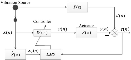
Figure 1.
A general block diagram of the Filtered-x Least Mean Square (FXLMS) algorithm.
The FXLMS algorithm performs an adaptation process on the controller weight vector (in this paper, the lowercase x, w, s, etc. are the time-domain representations of their respective frequency-domain counterparts) to minimize the instantaneous power of the residual vibration signal . According to the FXLMS algorithm, the output signal and the update equation of can be drawn as:
where is the secondary path impulse response, is an estimated FIR model of with L taps, and represent the controller weight vector in the th and th iteration, and is an adaption step size, which affects the stability and the convergence rate of the FXLMS algorithm and should be selected carefully.
When the output signal produced by the FXLMS algorithm exceeds the maximal allowed value , the rescaling algorithm clips the output signal and rescales the controller weight vector into the constraint set to obtain a new updated vector. The implementation process of the rescaling algorithm is:
(1) if , the rescaling algorithm has no effect on the normal FXLMS algorithm;
(2) if , the output signal and the controller weight vector are clipped and rescaled by the equations:
The rescaling algorithm is designed for a single-frequency output constraint and the total control power constraint in a sense. Although it has many advantages such as a high accuracy and flexibility compared with the leakage LMS algorithm, it has some shortages. The most important one is that a certain amount of high-order harmonic signals may be introduced into the system in multi-frequency cases [16]. Qiu used the allowed maximal amplitude in the theoretical analysis, but the maximal allowed output value was eventually used in his experiments, most likely because of the real-time amplitude of the output signal not being explicitly produced in the FXLMS algorithm. Thus, an estimation of the amplitude is needed, and the accuracy of the estimation will cause a lot of concerns. Thus, it can be further optimized for narrowband AVC applications, especially for sub-frequency constraint cases. A modified rescaling algorithm subject to reduced harmonics and implemented sub-frequency constraints has been studied in Section 3.
3. Modified Rescaling Algorithm Development
3.1. The NFXLMS Algorithm with Amplitude Compensation
The NFXLMS algorithm is a variant algorithm of FXLMS subject to narrowband noise and vibration control. It combines the trigonometric formulas with the FXLMS algorithm and can reduce the control effort dramatically [22,23,24,25,26,27,28]. It not only benefits from the real-time applications but also facilitates the manipulation of the line spectrum for some special purposes, such as the active noise equalizer and line spectrum reshaping [29,30,31,32,33]. The diagram of the NFXLMS algorithm is shown in Figure 2.
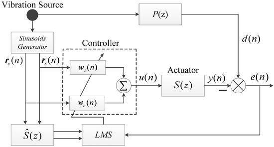
Figure 2.
The diagram of the NFXLMS algorithm.
Suppose the vibration source contains N frequency components , the normalized circular frequency vector is:
where and are the ith frequency component and ith normalized circular frequency, respectively. denotes the sample frequency. The two reference signal vectors are defined as:
where and denote the th cosine and sine reference signal, respectively. Accordingly, two controller weight vectors associated with the reference signal vectors are defined as:
Then, the output signal u(n) can be represented as:
where denotes the th component in the output signal corresponding to th frequency component. Similarly, the update equations of the weight vectors can be derived as [11,20,21,23]:
where is an estimated FIR model of with L taps as previously. Let and be the amplitude vector and the phase vector of the output signal . and can be calculated explicitly using trigonometric formulas as follows:
where denotes the th frequency component as previously. From Equation (9), it can be found that the secondary path introduces different amplitude ratios and phase differences at different frequencies. It causes the sub-frequency components to converge at different rates in the NFXLMS algorithm. In order to accelerate and balance the convergence rates of all sub-frequency components, an amplitude compensation method that multiplies the reference signal pairs by the normalized maximal amplitude ratio has been used [28,29,30,31]. Define the amplitude of the secondary path at each frequency component as:
where is the amplitude response of the secondary path model at the normalized circular frequency . Take the compensation matrix as:
The compensated reference signal vectors are:
Applying the compensated reference vectors to the NFXLMS algorithm, the two updated equations of the controller weight vectors change to the following form:
After compensating, the th frequency component of the output signal and the th element of the amplitude vector and phase vector can be calculated by the following equations, respectively:
3.2. Applying the Modified Rescaling Algorithm
Since the amplitude vector can be calculated analytically in the NFXLMS algorithm, it is convenient to apply the rescaling algorithm in order to apply the amplitude constraints to the target sub-frequency components. Here, the maximally allowed amplitude , rather than the maximally allowed value , is chosen as the constraint of the th frequency component. Define the output constraint vector:
where is the th amplitude constraint for the th frequency component. Then, the implementation process of the modified rescaling algorithm can be described in the following steps:
(1) Applying the compensated NFXLMS algorithm to produce the output signal component and calculate amplitude for all sub-frequencies by using Equations (15) and (16);
(2) Comparing the amplitude vector with the output constraint vector . If exists, then the th output component and the th controller weight pairs and are rescaled by the following equations:
(3) Summing up all the output components, the output signal after rescaling can be obtained as:
The modified rescaling algorithm retains the accuracy and flexibility of the original algorithm with new advantages. Constraints can be easily applied to the target sub-frequency components independently. The explicit amplitude constraint can also avoid potential clipping and improve the steady state of the output signal components at target frequencies. This means that less distortion and harmonics will be introduced into the control system.
3.3. Stability Analysis
Apparently, the proposed algorithm is the same as the NFXLMS algorithm before amplitude rescaling is triggered. When the amplitude rescaling of the th frequency component is triggered, the th output component can easily be drawn, as follows according to Equations (15)–(17):
Equation (21) shows that the amplitude will be restricted at the constraint while the phase can still be tuned by the NFXLMS algorithm. According to Equation (10), the ratio part eliminates the rescaling factor . This means that the phase-tuning process will not be affected by the rescaling algorithm and is the same as the compensated NFXLMS algorithm. Thus, the conditions that guarantee the stability of the compensated NFXLMS algorithm are sufficient conditions for the stability of the modified rescaling algorithm. The stability and robustness analysis of the related NFXLMS algorithm is fully studied and is outside the scope of this paper.
4. Simulation Study
4.1. Simulation Setup
A SDOF (single-degree of freedom) active vibration isolation platform model using an electromagnetic actuator has been chosen for the numerical simulation research [34,35,36,37,38]. The platform model is shown in Figure 3. is the disturbance force acting on the base. It is detected by the sensor as a vibration signal and fed into the controller. and are the response force of and the control force generated by the AVC system. is the residual vibration detected at the test point by an accelerometer sensor. The meanings and values of the rest parameters are illustrated in Table 1. The secondary path from the drive signal to the acceleration response at the test point on mass m can be derived as Formula (22) [21]. Then, is transformed into the Z-domain as by using the zero-order hold method and a sample time of = 0.001 s (or a sample frequency = 1000 Hz), as shown in Formula (23). An FIR model with 128 taps has been estimated offline using the LMS system identification method with adaptation step size and a delay = 1at sample frequency [20,21,22,38]. The bode diagrams of and are shown in Figure 4. To simplify, the primary path is set to 1 in the simulation. The adaption step size and vibration source will be chosen according to different purposes.
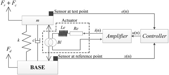
Figure 3.
A SDOF active vibration isolation platform model based on an electromagnetic actuator.

Table 1.
Parameters of the isolation platform for the simulation.
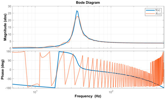
Figure 4.
The bode diagram of the simulation models and .
4.2. Case I: Simulation for Single-Frequency Vibration Control
A simulation for a single-frequency AVC with an output constraint has been accomplished at sample time . The disturbance signal is chosen to be with a white noise (RMS = 0.1 ). The simulation conditions are set as: (a) no control apllied; (b) with constraint = 10 V, with 10 V being far bigger than the value that rejects to zero under the ideal conditions and representing no constraint here; (c) with constraint 0.2 V; and (d) with constraint = 0.1 V, respectively. The adaption step size is set as =. The simulation results using the proposed algorithm are shown in Figure 5, Figure 6 and Figure 7.
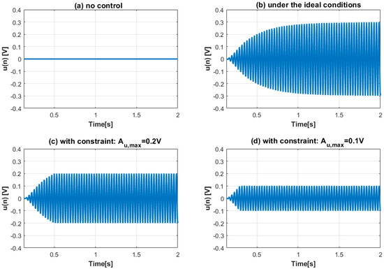
Figure 5.
The time-domain curve of the drive under different conditions: (a) no control; (b) under the ideal conditions; (c) with a constraint ; and (d) with a constraint .
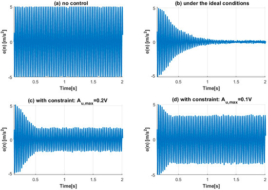
Figure 6.
The time-domain curve of the residual vibration under different conditions: (a) no control; (b) under the ideal conditions; (c) with a constraint ; and (d) with a constraint .
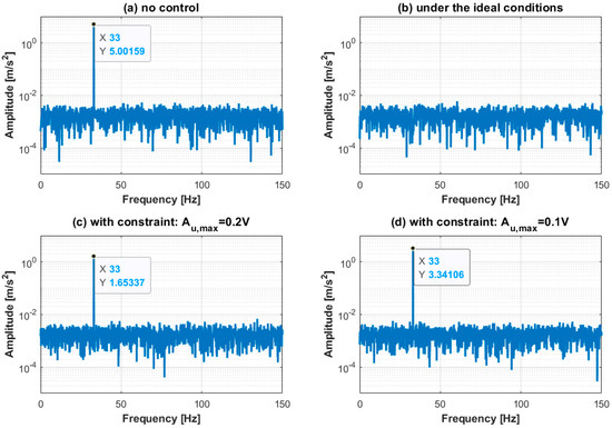
Figure 7.
The spectrum of the residual vibration under different conditions: (a) no control; (b) under the ideal conditions; (c) with a constraint ; and (d) with a constraint .
Figure 5 shows the simulation results of the output signal ’s time curve under different conditions: in Figure 5a no control is applied, which means = 0; in Figure 5b, the amplitude of the output signal grows to about 0.297 V under the ideal conditions via the NFXLMS algorithm; Figure 5b,c depicts that the amplitude of the output signal has been accurately restricted under the constraints = {0.2 V,0.1 V}. The relative errors of the control result are 1.5% and 1.35%, respectively. Figure 6 shows the time curve of the residual vibration under different conditions. Figure 6b depicts that the NFXLMS algorithm can reject the residual vibration to almost zero under ideal conditions while the constraints can maintain at a certain level in Figure 6c,d. The smoothness of the proposed algorithm triggering process can also be seen in Figure 6. The spectrum of the residual vibration at a steady state is shown in Figure 7. Figure 7c,d depicts that no significant harmonics are introduced to the control system.
4.3. Case II: Simulation for Multi-Frequency Constraints Control
Then, a simulation for a multi-frequency AVC with an output constraint control is studied at sample time . A disturbance signal that contains four frequency components has been chosen: = 22 Hz, = 31 Hz, = 55 Hz, and = 120 Hz. Their amplitude and initial phase are set as [1, 5, 5, 5] (unit: ) and [2*, 2*, 2*, 2*] (unit: degree), respectively. A white noise (RMS = 0.1 ) is added to the disturbance signal, as previously. The adaption step size is set to . The output constraint vector is set as = {10, 0.4, 0.2, 0} (unit: V). Thus, the goals of the simulation can be explained as: (a) rejecting the low-frequency component = 15 by setting the constraint = 10 V (means no constraint applied to ); (b) supposing that = 31 Hz is a key frequency and allocating more of the actuator’s power at by setting = 0.4 V; (c) supposing that = 55 Hz has a small impact and allocating less power by setting = 0.2 V; (d) supposing that the frequency component = 120 Hz is not concerned and then leaving it alone by setting = 0. To compare and illustrate the effect of compensations, the normal NFXLMS algorithm and the NFXLMS with compensation only are accomplished. The results are shown in Figure 8, Figure 9, Figure 10 and Figure 11.
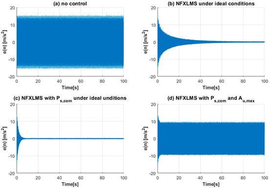
Figure 8.
The time-domain curve of the residual vibration using different variants of NFXLMS algorithms.
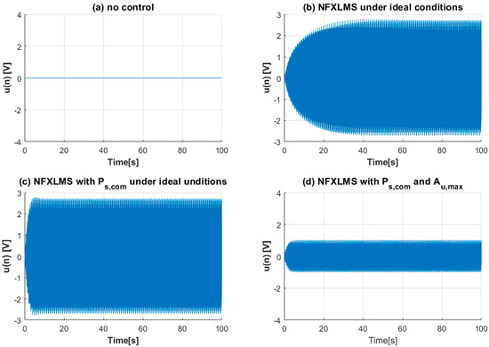
Figure 9.
The time-domain curve of the output signal using different variants of NFXLMS algorithms.
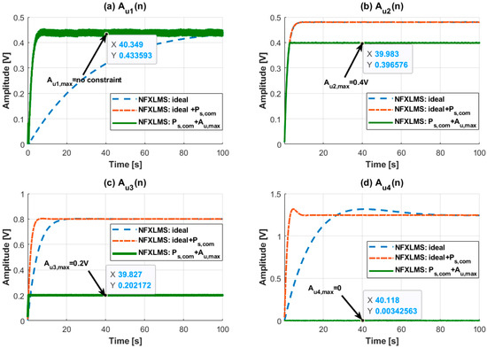
Figure 10.
The convergence curve of each sub-frequency’s amplitude in vector .
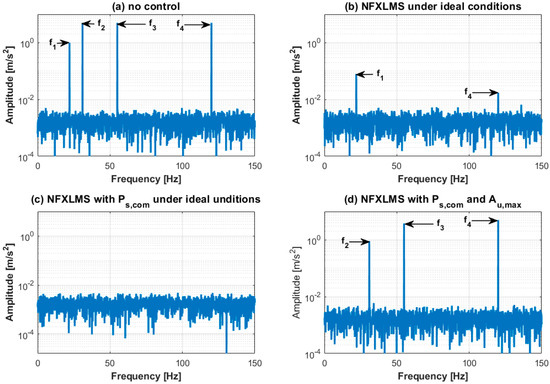
Figure 11.
The spectrum of the residual vibration after the AVC process at time intervals of [90s, 100s] using different variants of NFXLMS algorithms.
Figure 8 and Figure 9 shows the time curves of the residual vibration and output signal , respectively. The effect of the amplitude compensation is illustrated by comparing (b) with (c) in view of the control result and output in Figure 8 and Figure 9. In Figure 8d and Figure 9d, the proposed algorithm has kept the output signal and residual vibration to a certain level. Figure 10 shows the time curves of all the four sub-frequency component’s amplitudes. It can be found that four sub-frequency components achieved almost the same growth rate after compensating and that the constraints had been well implemented. Thus, the control goals according to have been achieved. Figure 11 shows the spectrum of the residual vibration after the AVC process at 90~100 s. In Figure 11b, there are still two small-scale frequency components, = 22 Hz and = 120 Hz, that have not been totally rejected due to the low convergence rate, while the NFXLMS with compensation has rejected all the frequencies to zero when compared with Figure 11c. In Figure 11d, almost no harmonics are introduced to the control system, as in the single frequency case.
5. Conclusions and Discussions
This paper proposed a modified rescaling algorithm to implement a frequency-selective output constraint control for active vibration control. It not only retains the features of accuracy and flexibility of the original rescaling algorithm but also has new advantages and features such as having less distortion and harmonics, being suited for individual sub-frequency components’ amplitude constraint and optimal control power allocating, etc. Thus, the proposed algorithm is very practical for AVC applications in order to improve safety and optimal control when the limits of actuators have to be taken into account. Simulations conducted with single-frequency and multi-frequency cases demonstrated its effectiveness, accuracy, and flexibility.
Although the algorithm presented in this paper is well studied, there are still some areas open to further research. There are some other projection algorithms such as the affine-scaling algorithm can be used to replace the rescaling method in order to accelerate the convergence rate. Correspondingly, in narrow-band vibration applications, those algorithms could be further studied. Furthermore, in some applications, it may be necessary to dynamically adjust the constraint values at some target frequencies rather than constant constraints. The impact of dynamic constraint values on the stability of the NFXLMS algorithm should be studied next.
Author Contributions
Investigation, X.M. and Z.C.; Validation, Z.C.; Writing—original draft, X.M.; Writing—review & editing, X.M. and Z.C. All authors have read and agreed to the published version of the manuscript.
Funding
This research received no external funding.
Data Availability Statement
All data included in this study are available upon request by contact with the author Xibin Ma.
Conflicts of Interest
The authors declare no conflict of interest.
References
- Connolly, C. Vibration isolation theory and practice. Assem. Autom. 2009, 29, 8–13. [Google Scholar] [CrossRef]
- Ferrer, M.; De Diego, M.; Pinero, G.; Gonzalez, A. Active noise control over adaptive distributed networks. Signal Process. 2015, 107, 82–95. [Google Scholar] [CrossRef]
- Sun, G.; Feng, T.; Li, M.; Lim, T.C. Convergence analysis of FxLMS-based active noise control for repetitive impulses. Appl. Acoust. 2015, 89, 78–187. [Google Scholar] [CrossRef]
- Li, Z.; Jiang, Y.; Hu, C. Recent progress on decoupling diagnosis of hybrid failures in gear transmission systems using vibration sensor signal: A review. Measurement 2016, 90, 4–19. [Google Scholar] [CrossRef]
- Adam, G. Acoustic based fault diagnosis of three-phase induction motor. Appl. Acoust. 2018, 137, 82–89. [Google Scholar] [CrossRef]
- Glowacz, A. Fault diagnosis of single-phase induction motor based on acoustic signals. Mech. Syst. Signal Process. 2019, 117, 65–80. [Google Scholar] [CrossRef]
- Li, Z.; Jiang, Y.; Hu, C.; Peng, Z. Difference equation based empirical mode decomposition with application to separation enhancement of multi-fault vibration signals. J. Differ. Equ. Appl. 2017, 23, 457–467. [Google Scholar] [CrossRef]
- Bjarnason, E. Analysis of the filtered-X LMS algorithm. Speech Audio Process. IEEE Trans. 1993, 3, 504–514. [Google Scholar] [CrossRef]
- Tobias, O.J.; Bermudez, J.C.M.; Bershad, N.J.; Seara, R. Mean weight behavior of the Filtered-X LMS algorithm. In Proceedings of the 1998 IEEE International Conference on Acoustics, Speech and Signal Processing, Seattle, WA, USA, 12–15 May 1998; pp. 3545–3548. [Google Scholar] [CrossRef]
- Tobias, O.J.; Bermudez, J.C.M.; Bershad, N.J. Mean weight behavior of the Filtered-X LMS algorithm. IEEE Trans. Signal Process. 2000, 48. [Google Scholar] [CrossRef]
- Kuo, S.M.; Morgan, D.R. Active Noise Control Systems, Algorithms and DSP Implementations; Wiley: New York, NY, USA, 1996. [Google Scholar]
- Elliott, S.J.; Back, K.H. Effort constraints in adaptive feedforward control. IEEE Signal Process. Lett. 1996, 3, 7–9. [Google Scholar] [CrossRef]
- Douglas, S.C. Performance comparison of two implementations of the leaky LMS adaptive filter. IEEE Trans. Signal Process. 1997, 45, 2125–2129. [Google Scholar] [CrossRef]
- Rafaely, B.; Elliot, S.J. A computationally efficient frequency-domain LMS algorithm with constraints on the adaptive filter. IEEE Trans. Signal Process. 2000, 48, 1649–1655. [Google Scholar] [CrossRef]
- Qiu, X.; Hansen, C.H. A study of time-domain FXLMS algorithms with control output constraint. J. Acoust. Soc. Am. 2001, 109, 2815–2823. [Google Scholar] [CrossRef] [PubMed]
- Hao, C.; Yong, W.; Jia-quan, L.; Yang, L. Research on the Control of Electromagnetic Suspension Vibration Isolator based on LMS Algorithm with Saturation Constraint. J. Vib. Shock 2012, 31, 125–128. [Google Scholar] [CrossRef]
- Qiu, X.; Hansen, C.H. Applying effort constraints on adaptive feedforward control using the active set method. J. Sound Vib. 2003, 260, 757–762. [Google Scholar] [CrossRef]
- Kozacky, W.J.; Ogunfunmi, T. An active noise control algorithm with gain and power constraints on the adaptive filter. ERUASIP J. Adv. Signal Process. 2013, 17. [Google Scholar] [CrossRef]
- Shi, D.Y.; Gan, W.-S.; Lam, B.; Shi, C. Two-gradient direction FXLMS: An adaptive active noise control algorithm with output constraint. Mech. Syst. Signal Process. 2018, 116, 651–667. [Google Scholar] [CrossRef]
- Farhang-Boroujeny, B. Adaptive Filters: Theory and Applications; Wiley: New York, NY, USA, 2013. [Google Scholar]
- Haykin, S. Adaptive Filter Theory, 4th ed.; Prentice Hall: Upper Saddle River, NJ, USA, 2002. [Google Scholar]
- Glover, J. Adaptive noise canceling applied to sinusoidal interferences. IEEE Trans. Acoust. Speech Signal Process. 1978, 25, 484–491. [Google Scholar] [CrossRef]
- Wang, L.; Gan, W.S. Analysis of misequalization in a narrowband active noise equalizer system. J. Sound Vib. 2008, 311, 1438–1446. [Google Scholar] [CrossRef]
- Wang, L.; Gan, W.S. Convergence Analysis of Narrowband Active Noise Equalizer System Under Imperfect Secondary Path Estimation. IEEE Trans. Audio Speech Lang. Process. 2009, 17, 566–571. [Google Scholar] [CrossRef]
- Xiao, Y.; Ikuta, A.; Ma, L.; Khorasani, K. Stochastic Analysis of the FXLMS-Based Narrowband Active Noise Control System. IEEE Trans. Audio Speech Lang. Process. 2008, 16, 1000–1014. [Google Scholar] [CrossRef]
- Xiao, Y. A New Robust Narrowband Active Noise Control System in the Presence of Frequency Mismatch. IEEE Trans. Audio Speech Lang. Process. 2006, 14. [Google Scholar] [CrossRef]
- Sun, C.; Liu, Y.; Bo, Z.; Jiang, S. A New Online Secondary Path Modeling Method with An Auxiliary Noise Power Scheduling Strategy for Narrowband Active Noise Control Systems. Appl. Sci. 2017, 7, 1236. [Google Scholar] [CrossRef]
- Chang, C.Y.; Kuo, S.M.; Huang, C.W. Secondary path modeling for narrowband active noise control systems. Appl. Acoust. 2018, 131, 154–164. [Google Scholar] [CrossRef]
- Liu, J.; Chen, X.; Yang, L.; Gao, J.; Zhang, X. Analysis and compensation of reference frequency mismatch in multiple-frequency feedforward active noise and vibration control system. J. Sound Vib. 2017, 409, 145–164. [Google Scholar] [CrossRef]
- Liu, J.; Chen, X. Adaptive Compensation of Misequalization in Narrowband Active Noise Equalizer Systems. IEEE/ACM Trans. Audio Speech Lang. Process. 2016, 24, 2390–2399. [Google Scholar] [CrossRef]
- Liu, J.; Chen, X.; Gao, J.; Zhang, X. Multiple-source multiple-harmonic active vibration control of variable section cylindrical structures: A numerical study. Mech. Syst. Signal Process. 2016, 81, 461–474. [Google Scholar] [CrossRef]
- Gong, Y.; Song, Y.; Liu, S. Performance analysis of the unconstrained FxLMS algorithm for active noise control. In Proceedings of the 2003 IEEE International Conference on Acoustics, Speech, and Signal Processing, Hong Kong, China, 6–10 April 2003. [Google Scholar] [CrossRef]
- Jeon, H.J.; Chang, T.G.; Kuo, S.M. Analysis of Frequency Mismatch in Narrowband Active Noise Control. Audio Speech Lang. Process. IEEE Trans. 2010, 18, 1632–1642. [Google Scholar] [CrossRef]
- Wu, F.Y.; Tong, F. Gradient optimization p-norm-like constraint LMS algorithm for sparse system estimation. Signal Process. 2013, 93, 967–971. [Google Scholar] [CrossRef]
- Stefano, C.; Maryam, G.T.; John, E.S. Parametric study on the optimal tuning of an inertial actuator for vibration control of a plate: Theory and experiments. J. Sound Vib. 2018, 435, 1–22. [Google Scholar] [CrossRef]
- Dal Borgo, M.; Tehrani, M.G.; Elliott, S.J. Identification and analysis of nonlinear dynamics of inertial actuators. Mech. Syst. Signal Process. 2019, 115, 338–360. [Google Scholar] [CrossRef]
- Elliott, S.J.; Zilletti, M. Scaling of electromagnetic transducers for shunt damping and energy harvesting. J. Sound Vib. 2014, 333, 2185–2195. [Google Scholar] [CrossRef]
- Lichota, P.; Szulczyk, J.; Tischler, M.B.; Berger, T. Frequency Responses Identification from Multi-Axis Maneuver with Simultaneous Multisine Inputs. J. Guid. Control Dyn. 2019, 42, 2550–2556. [Google Scholar] [CrossRef]
Publisher’s Note: MDPI stays neutral with regard to jurisdictional claims in published maps and institutional affiliations. |
© 2020 by the authors. Licensee MDPI, Basel, Switzerland. This article is an open access article distributed under the terms and conditions of the Creative Commons Attribution (CC BY) license (http://creativecommons.org/licenses/by/4.0/).