Converting MST to TSP Path by Branch Elimination

Abstract

Travelling salesman problem (TSP) has been widely studied for the classical closed loop variant but less attention has been paid to the open loop variant. Open loop solution has property of being also a spanning tree, although not necessarily the minimum spanning tree (MST). In this paper, we present a simple branch elimination algorithm that removes the branches from MST by cutting one link and then reconnecting the resulting subtrees via selected leaf nodes. The number of iterations equals to the number of branches (b) in the MST. Typically, b << n where n is the number of nodes. With O-Mopsi and Dots datasets, the algorithm reaches gap of 1.69% and 0.61 %, respectively. The algorithm is suitable especially for educational purposes by showing the connection between MST and TSP, but it can also serve as a quick approximation for more complex metaheuristics whose efficiency relies on quality of the initial solution.

1. Introduction

The classical closed loop variant of travelling salesman problem (TSP) visits all the nodes and then returns to the start node by minimizing the length of the tour. Open loop TSP is slightly different variant, which skips the return to the start node. They are both NP-hard problems [1], which means that finding optimal solution fast can be done only for very small size inputs.

The open loop variant appears in mobile-based orienteering game called O-Mopsi (http://cs.uef.fi/o-mopsi/) where the goal is to find a set of real-world targets with the help of smartphone navigation [2]. This includes three challenges: (1) Deciding the order of visiting the targets, (2) navigating to the next target, and (3) physical movement. Unlike in classical orienteering where the order of visiting the targets is fixed, O-Mopsi players optimize the order while playing. Finding the optimal order is not necessary but desirable if one wants to minimize the tour length. However, the task is quite challenging for humans even for short problem instances. In [2], only 14% of the players managed to solve the best order among those who completed the tour. Most players did not even realize they were dealing with TSP problem.

Minimum spanning tree (MST) and TSP are closely related algorithmic problems. In specific, open loop TSP solution is also a spanning tree but not necessarily the minimum spanning tree; see Figure 1. The solutions have the same number of links (n $-$ 1) and they both minimize the total weight of the selected links. The difference is that TSP does not have any branches. This connection is interesting for two reasons. First, finding optimal solution for TSP requires exponential time while optimal solution for MST can be found in polynomial time using greedy algorithms like Prim and Kruskal, with time complexity very close to O(n²) with appropriate data structure.

The connection between the two problems have inspired researchers to develop heuristic algorithms for the TSP by utilizing the minimum spanning tree. Classical schoolbook algorithm is Christofides [3,4], which first creates an MST. More links are then added so that the Euler tour can be constructed. Travelling salesman tour is obtained from the Euler tour by removing nodes that are visited repeatedly. This algorithm is often used as classroom example because it provides upper limit how far the solution can be from the optimal solution in the worst case. Even if the upper limit, 50%, is rather high for real life applications, it serves as an example of the principle of approximation algorithms.

MST has also been used to estimate lower limit for the optimal TSP solution in [5], and to estimate the difficulty of a TSP instance by counting the number of branches [6]. Prim’s and Kruskal’s algorithms can also been modified to obtain sub-optimal solutions for TSP. Class of insertion algorithms were studied in [7]. They iteratively add new nodes to the current path. The variant that adds a new node to either end of the existing path can be seen as modification of the Prim’s algorithm where additions are allowed only to the ends of the path. Similarly, algorithm called Kruskal-TSP [8] modifies Kruskal’s algorithm so that it allows to merge two spanning trees (paths in case of TSP) only by their end points.

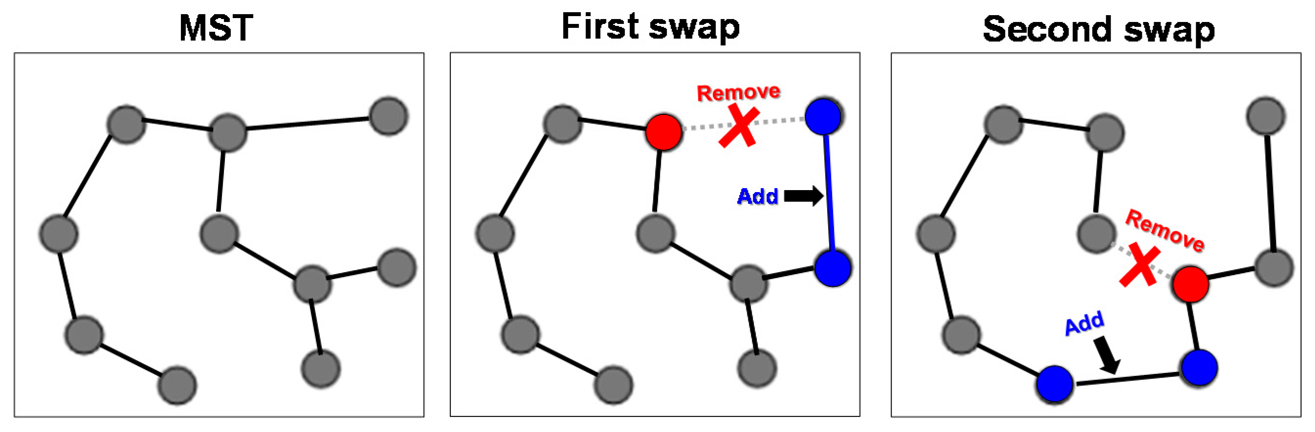
In this paper, we introduce a more sophisticated approach to utilize the minimum spanning tree to obtain solution for travelling salesman problem. The algorithm, called MST-to-TSP, creates a minimum spanning tree using any algorithm such as Prim or Kruskal. However, instead of adding redundant links like Chirstofides, we detect branching nodes and eliminate them by a series of link swaps, see Figure 2. Branching node is a node that connects more than two other nodes in the tree [6]. We introduce two strategies. First, a simple greedy variant removes the longest of all links connecting to any of the branching nodes. The resulting sub-trees are then reconnected by selecting the shortest link between leaf nodes. The second strategy, all-pairs, considers all possible removal and reconnection possibilities and selects the best pair.

We test the algorithm with two datasets consisting of open loop problem instances with known ground truth: O-Mopsi [2] and Dots [9]. Experiments show that the all-pairs variant provide average gaps of 1.69% (O-Mopsi) and 0.61% (Dots). These are clearly better than those of the existing MST-based variants including Christofides (12.77% and 9.10%), Prim-TSP (6.57% and 3.84%), and Kruskal-TSP (4.87% and 2.66%). Although sub-optimal, the algorithm is useful to provide reasonable estimate for the TSP solution. It is also not restricted to complete graphs with triangular inequality like Christofides. In addition, we also test repeated randomized variant of the algorithm. It reaches results very close to the optimum; averages of 0.07% (O-Mopsi) and 0.02% (Dots).

One of the main motivations for developing heuristics algorithms earlier has been to have a polynomial time approximation algorithm for TSP. Approximation algorithms guarantee that the gap between the heuristic and optimal results has a proven upper limit but these limits are usually rather high: 67% [10], 62% [11], 50% [4], 50%-ε [12], and 40% [13]. The variant in [14] was speculated to have limit as low as 25% based on empirical observations. The results generalize to the open-loop case so that if there exists α-approximation for the closed-loop TSP there exists α+ε approximation for the open-loop TSP [15,16]. However, for practical purpose, all of these are high. Gaps between 40% to 67% are likely to be considered insufficient for industrial applications.

The second motivation for developing heuristic algorithms is to provide initial solution for more complex algorithms. For example, the efficiency of local search and other metaheuristics highly depends on the initial solution. Starting from a poor-quality solution can lead to much longer iterations, or even prevent reaching a high-quality solution with some methods. Optimal algorithms like branch-and-cut also strongly depend on the quality of initialization. The better the starting point, the more can be cut out by branch-and-cut. One undocumented rule of thumb is that the initial solution should be as good as ~1% gap in order to achieve significant savings compared to exhaustive search.

The rest of the paper is organized as follows. Section 2 reviews the existing algorithms focusing on the those based on minimum spanning tree. The new MST-to-TSP algorithm is then introduced in Section 3. Experimental results are reported in Section 4 and conclusions drawn in Section 5.

2. Heuristic Algorithms for TSP

We review the common heuristic found in literature. We consider the following algorithms:

• Nearest neighbor [17,18].
• Greedy/Prim-TSP [17,18].
• Kruskal-TSP [8].
• Christofides [3,4].
• Cross removal [19].

Nearest neighbor (NN) is one of the oldest heuristic methods [17]. It starts from random node and then constructs the tour stepwise by always visiting the nearest unvisited node until all nodes have been reached. It can lead to inferior solutions like 25% worse than the optimum in the example in Figure 3. The nearest neighbor strategy is often applied by human problem solvers in real-world environment [6]. A variant of nearest neighbor in [18] always selects the shortest link as long as new unvisited nodes are found. After that, it switches to the greedy strategy (see below) for the remaining unvisited nodes. In [9], the NN-algorithm is repeated N times starting from every possible node, and then selecting the shortest tour of all n alternatives. This simple trick would avoid the poor choice shown in Figure 3. In [14], the algorithm is repeated using all possible links as the starting point instead of all possible nodes. This increases the number of choices up to n*(n-1) in case of complete graph.

Greedy method [17,18] always selects the unvisited node having shortest link to the current tour. It is similar to the nearest neighbor except that it allows to add the new node to both ends of the existing path. We call this as Prim-TSP because it constructs the solution just like Prim except it does not allow branches. In case of complete graphs, nodes can also be added in the middle of the tour by adding a detour via the newly added node. A class of insertion methods were studied in [7] showing that the resulting tour is no longer than twice of the optimal tour.

Kruskal-TSP [8] also constructs spanning tree like Prim-TSP. The difference is that while Prim operates on a single spanning tree, Kruskal operates on a set of trees (spanning forest). It therefore always selects the shortest possible link as long as they merge to different spanning trees. To construct TSP instead of MST, it also restricts the connections only to the end points. However, while Prim-TSP has only two possibilities for the next connection, Kruskal-TSP has potentially much more; two for every spanning tree in the forest. It is therefore expected to make fewer sub-optimal selections, see Figure 4 for an example. The differences between NN, Prim-TSP, and Kruskal-TSP are illustrated in Figure 5.

Classical Christofides algorithm [3,4] includes three steps: (1) Create MST, (2) add links and create Euler tour, and (3) remove redundant paths by shortcuts. Links are added by detecting nodes with odd degree and creating new links between them. If there are n nodes with odd degree (odd nodes), then n/2 new links are added. To minimize the total length of the additional links, perfect matching can be solved by Blossom algorithm, for instance [20]. Example of Christofides is shown in Figure 6. In [12], a variant of Christofides was proposed by generating alternative spanning tree that has higher cost than MST but fewer odd nodes. According to [21], this reduces the number of odd nodes from 36–39% to 8–12% in case of TSPLIB and VLSI problem instances.

Most of the above heuristics apply both to the closed-loop and open-loop cases. Prim and Kruskal are even better suited for the open-loop cases as the last link in the closed loop case is forced and is typically a very long, sub-optimal choice. Christofides, on the other hand, was designed strictly for the closed-loop case due to the creation of the Euler tour. It therefore does not necessarily work well for the open-loop case, which can be significantly worse.

There are two strategies how to create open-loop solution from a closed-loop solution. A simple approach is to remove the longest link, but this does not guarantee an optimal result; see Figure 7. Another strategy is to create additional pseudo node, which has equal (large) distance to all other nodes [9]. Any closed-loop algorithm can then be applied, and the optimization will be performed merely based on the other links except those two that will be connecting to the pseudo node which are all equal. These two will be the start and end nodes of the corresponding open-loop solution. If the algorithm provides optimal solution for the closed-loop problem, it was shown to be optimal also for the corresponding open-loop case [1].

However, when heuristic algorithm is applied, the pseudo node strategy does may not always work as expected. First, if the weights to the pseudo node are small (e.g., zeros), then algorithms like MST would links all nodes to the pseudo node, which would make no sense for Christofides. Second, if we choose large weights to the pseudo node, it would be connected to MST last. However, as the weights are all equal, the choice would be arbitrary. As a result, the open loop case will not be optimized any better if we used the pseudo node than just removing the longest link. Ending up with a good open-loop solution by Christofides seems merely a question of luck. Nevertheless, we use the pseudo node strategy as it is the de facto standard due to it guaranteeing optimality for the optimal algorithm at least.

The existing MST-based algorithms take one of the two approaches: (1) Modify the MST solution to obtain TSP solution [3,4]; (2) modify the existing MST algorithm to design algorithm for TSP [7,8,16,17]. In this paper, we follow the first approach and take the spanning tree as our starting point.

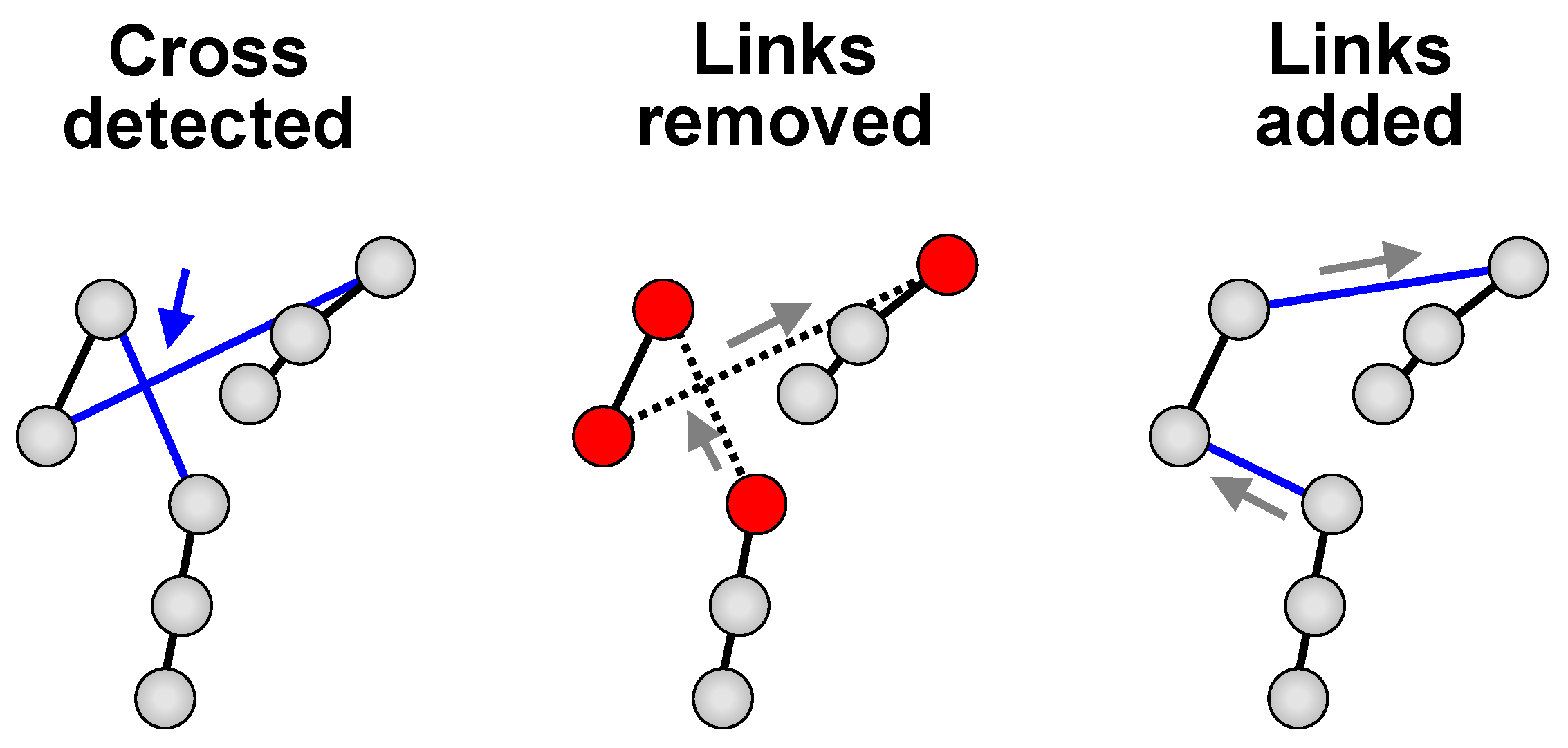
Among other heuristics we mention local search. It aims at improving an existing solution by simple operators. One obvious approach is Cross removal [19], which is based on the fact that optimal tour cannot cross itself. The heuristic simply detects any cross along the path, and if found, eliminates it by re-connecting the links involved as shown in Figure 8. It can be shown that the cross removal is a special case of the more general 2-opt heuristic [22]. Another well-known operator is relocation that removes a node from the path and reconnects it to another part of the path. The efficiency of several operators has been studied in [9] within an algorithm called Randomized mixed local search.

While local search is still the state-of-the-art and focus has been mainly on operators such as 2-opt and its generalized variant k-opt [23,24], other metaheuristics have been also considered. These include tabu search [25], simulated annealing and combined variants [26,27,28], genetic algorithm [29,30], ant colony optimization [31], and harmony search [32].

3. MST-to-TSP Algorithm

The proposed algorithm resembles Christofides as it also generates minimum spanning tree to give first estimate of the links that might be needed in TSP. Since we focus on the open-loop variant, it is good to notice that the TSP solution is also a spanning tree, although not the minimum one. However, while Christofides adds redundant links to create Euler tour, which are then pruned by shortcuts, we do not add anything. Instead, we change existing links by a series of link swaps. In specific, we detect branches in the tree and eliminate them one by one. This is continued until the solution becomes a TSP path; i.e., spanning tree without any branches. Pseudo codes of the variants are sketched in Algorithm1 and Algorithm2.

Algorithm 1: Greedy variant

MST-to-TSP(X) → TSP:   T ← GenerateMST(X);   WHILE branches DO     e1 ← LongestBranchLink(T);     e2 ← ShortestConnection(T);     T ← SwapLink(T, e1, e2);   RETURN(T);

Algorithm 2:All-pairs variant

MST-to-TSP(X) → TSP:   T ← GenerateMST(X);   WHILE branches DO     e1, e2← OptimalPair(T);     T ← SwapLink(e1, e2);   RETURN(T);

Both variants start by generating minimum spanning tree by any algorithm such as Prim and Kruskal. Prim grows the tree from scratch. In each step, it selects the shortest link that connects a new node to the current tree while Kruskal grows a forest by selecting shortest link that connects two different trees. Actually, we do not need to construct minimum spanning tree, but some sub-optimal spanning tree might also be suitable [33]. For Christofides, it would be beneficial to have a tree with fewer nodes with odd degree [12]. In our algorithm, having spanning tree with fewer branches might be beneficial. However, to keep the algorithm simple, we do not study this possibility further in this paper.

Both variants operate on the branches, which can be trivially detected during the creation of MST simply by maintaining the degree counter when links are added. Both algorithms also work sequentially by resolving the branches one by one. They differ only in the way the two links are selected for the next swap; all other parts of the algorithm variants are the same. The number of iterations equals the number of branches in the spanning tree. We will next study the details of the two variants.

3.1. Greedy Variant

The simpler variant follows the spirit of Prim and Kruskal in a sense that it is also greedy. The selection is split into two subsequent choices. First, we consider all links connecting to any branching node, and simply select the longest. This link is then removed. As a result, we will have two disconnected trees. Second, we reconnect the trees by considering all pairs of leaf nodes so that one is from the first subtree and the other from the second subtree. The shortest link is selected.

Figure 9 demonstrates the algorithm for a graph with n = 10 nodes. In total, there are two branching nodes and six links attached to them. The first removal creates subtrees of size n₁ = 9 (3 leaves) and n₂ = 1 (1 leaf) providing 3 possibilities for the re-connection. The second removal creates subtrees of size n₁ = 6 (2 leaves) and n₂ = 4 (2 leaves). The result is only slightly longer than the minimum spanning tree.

3.2. All-Pairs Variant

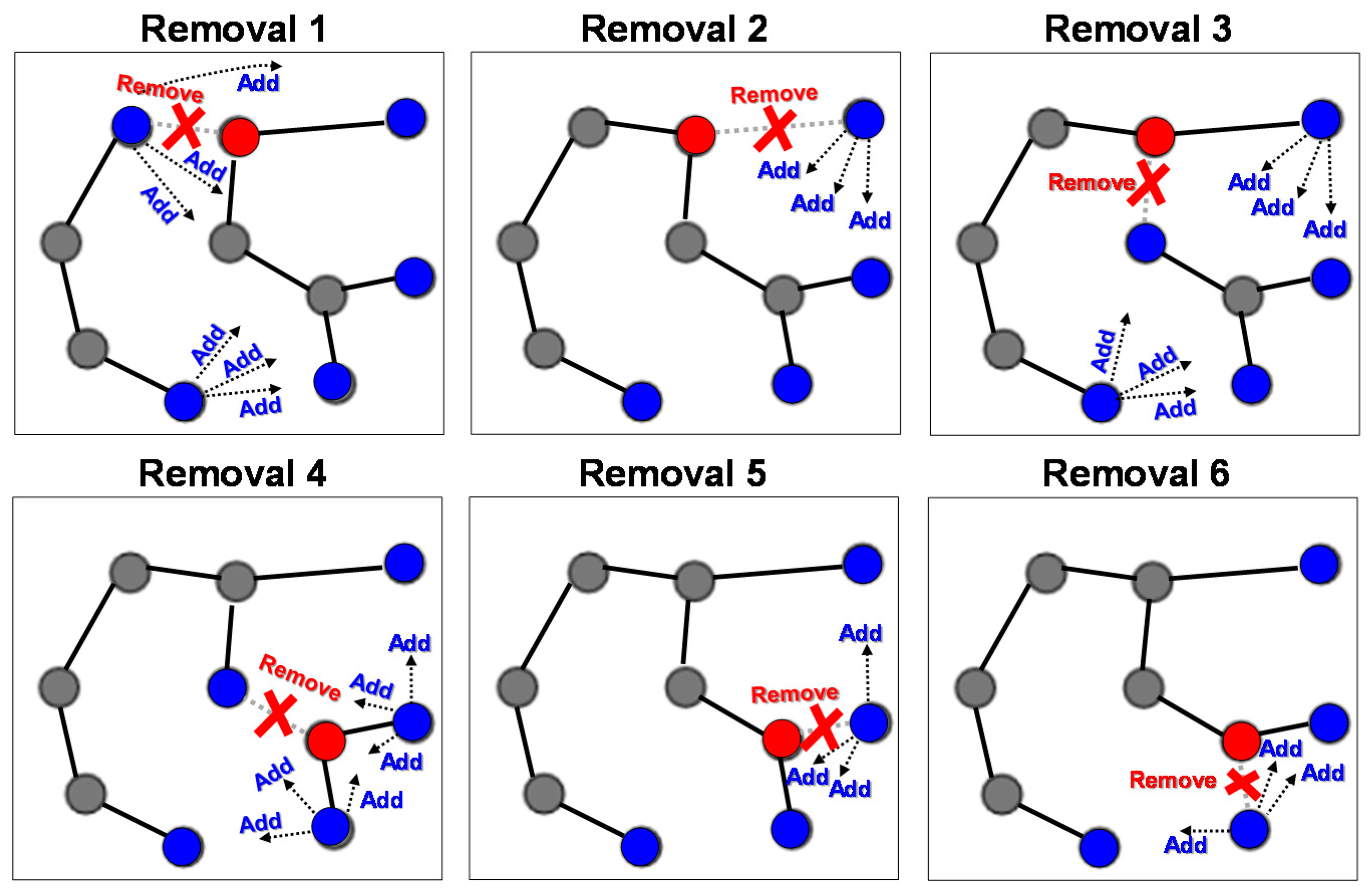
The second variant optimizes the removal and addition jointly by considering all pairs of links that would perform a valid swap. Figure 10 demonstrates the process. There are 6 removal candidates, and they each have 3–6 possible candidates for the addition. In total, we have 27 candidate pairs. We choose the pair that increases the path length least. Most swaps increase the length of the path but theoretically it is possible that some swap might also decrease the total path; this is rare though.

The final result is shown in Figure 11. With this example, the variant finds the same solution as the as the greedy variant. However, the parallel chains example in Figure 12 shows situation where the All-pairs variant works better than the greedy variant. Figure 13 summarizes the results of the main MST-based algorithms. Nearest neighbor works poorly because it depends on the arbitrary start point. If considered all possible start points, it would reach the same result as Prim-TSP, Kruskal-TSP and the greedy variant of MST-to-TSP. In this example, the all-pairs variant of MST-to-TSP is the only heuristic that finds the optimal solution, which includes the detour in the middle of the longer route.

There are (2 $·$ 3) + (1 $·$ 3) + (2 $·$ 3) + (2 $·$ 3) + (1 $·$ 3) + (1 $·$ 3) = 27 candidates in total.

3.3. Randomized Variant

The algorithm can be further improved by repeating it several times. This improvement is inspired by [34] where k-means clustering algorithm was improved significantly by repeating it 100 times. The only requirement is that the creation of the initial solution includes randomness so that it produces different results every time. In our randomized variant, the final solution is the best result out of the 100 trials. The idea was also applied for the Kruskal-TSP and called Randomized Kruskal-TSP [8].

There are several ways how to randomize the algorithm. We adopt the method from [8] and randomize the creation of MST. When selecting the next link for the merge, we randomly choose one out of the three shortest links. This results in sub-optimal choices. However, as we have a complete graph, it usually has several virtually as good choices. Furthermore, the quality of the MST itself is not a vital for the overall performance of the algorithm; the branch elimination plays a bigger role than the MST. As a result, we will get multiple spanning trees producing different TSP solutions. Out of the 100 repeats, it is likely that one provides better TSP than using only the minimum spanning tree as starting point.

4. Experimental Results

4.1. Datasets and Methods

We use two open loop datasets: O-Mopsi [2] and Dots [35]; see Figure 14. Both can be found on web: http://cs.uef.fi/o-mopsi/datasets/. O-Mopsi are 147 instances of mobile orienteering game played in real-world. Haversine distance is used with the constant 6356.752 km for the earth radius. The dots are 6449 computer-generated problem instances designed for humans to solve on computer screen. Euclidean distance is used. Optimal ground truth solutions are available for all problem instances.

Table 1. Datasets used in the experiments.

						Branches:
Dataset	Reference	Distance	Instances	N	Min	Average	Max
O-Mopsi	[2]	Haversine	147	4-27	0	1.90	5
Dots	[35]	Euclidean	6449	4-31	0	1.48	11

summarizes the properties of the datasets. On average, the datasets have only a few branches (1.90 in O-Mopsi; 1.48 in Dots). This means that that the MST-to-TSP algorithm needs to run only a few iterations. Even the most difficult Dots instance has only 11 branches to be broken. The total number of link swaps need are 280 for the O-Mopsi games and 9548 for the Dots games.

Table 2. Accuracy comparison of the algorithms (gap) for the two series of datasets.

Algorithm	Reference	Average		Worst
		O-Mopsi	Dots	O-Mopsi	Dots
Christofides	[3,4]	12.77%	9.10%	35.41%	39.21%
Nearest neighbor	[17]	20.00%	9.25%	66.57%	48.06%
Nearest neighbor+	[9]	3.47%	1.49%	21.01%	22.80%
Prim-TSP	[17]	6.57%	3.84%	32.95%	35.23%
Kruskal-TSP	[8]	4.87%	2.66%	28.59%	28.40%
Kruskal-TSP (100r)	[8]	0.77%	0.26%	7.13%	13.46%
MST-to-TSP (greedy)	(proposed)	4.81%	2.93%	21.98%	28.40%
MST-to-TSP (all-pairs)	(proposed)	1.69%	0.61%	16.32%	15.46%
MST-to-TSP (all-pairs 100r)	(proposed)	0.07%	0.02%	1.98%	2.42%
2-opt	[22]	1.72%	1.35%	15.53%	22.86%
Random Mix Local Search	[9]	0.00%	0.01%	0.27%	2.59%

shows the methods used in the experiments. We include all the main MST-based algorithms including nearest neighbor, Prim-TSP (greedy), Kruskal-TSP, and the proposed MST-to-TSP. Randomized variants are included from Kruskal-TSP and MST-to-TSP with 100 repeats. Among the local search heuristics, we include 2-opt [22] and the randomized mixed local search [9]. The performance is evaluated by gap, which is relative difference of the algorithm and optimal solutions:

$$gap=\frac{\left|L-L_{opt}\right|}{L_{opt}}$$

(1)

4.2. Results

Table 2 also shows the average results with the O-Mopsi and Dots data. From these we can learn a few things.

First, while the greedy variant of MST-to-TSP provides similar results to that of Kruskal-TSP (4.81% and 2.93%), the all-pairs variant is significantly better (1.69% and 0.61%) and the randomized version reaches near-optimal results (0.07% and 0.02%). In other words, it is clearly superior to the existing MST-based heuristics and very close to the more sophisticated local search (0.00% and 0.01%).

Second, by comparing the greedy we can see that the more options the algorithm has for the next merge, the better its performance. Nearest neighbor performs worst as it has only one possibility to continue from the previously added node. Prim-TSP always has two choices and performs better. Kruskal-TSP has often more options for the merge and is the best among these. Randomized Kruskal-TSP is already more competitive but still inferior to MST-to-TSP.

Third, Christofides reaches average values of 12.77% (O-Mopsi) and 9.10% (Dots), which are clearly the worst among all tested algorithms. Its advantage is that it is the only algorithm that provides guarantee (50%) for the worst case. However, with these datasets this is merely theoretical as most other heuristics never get worse than 50% anyway. The only advantage of Christofides is that this 50% upper limit is theoretically proven. For practice, MST-to-TSP is clearly better choice.

The dependency on the number of nodes is demonstrated in Figure 15. We can see that the gap tends to increase with the problem size. This is as expected but it remains an open question whether the gap value would converge to certain level with this type of 2-dimensional problem instances.

Table 3. Cost of the link swaps (meters) in MST-to-TSP during the algorithm with O-Mopsi data.

Swap	1	2	3	4	5
Max	1074	1192	497	1126	681
Average	108	155	145	227	381
Min	1	1	1	13	134
Count	130	84	47	16	3
%	31%	25%	21%	9%	2%

shows how the link swaps increase the length of the path when converting the spanning tree to TSP path. Out of the 147 O-Mopsi games, 19 (12%) have no branches and the minimum spanning tree is the optimal solution for TSP as such. Most other games have only one (31%) or two (25%) branches, which shows that the task of converting MST to TSP is not too difficult in most cases. Only about 10% of the games require more than two swaps.

Statistics for the Dots games are similar; see

Table 4. Cost of the link swaps in MST-to-TSP during the algorithm with Dots data.

Swap	1	2	3	4	5	6	7	8	9	10
Max	30.62	25.75	29.18	42.99	35.55	29.42	27.46	29.68	26.49	15.41
Average	5.65	5.98	5.95	5.94	6.74	6.83	6.71	6.60	10.76	11.01
Min	0.00	−4.12	−5.84	−6.43	0.00	0.00	0.04	0.00	1.90	3.26
Count	4525	2374	1169	622	341	171	87	43	17	6
%	33%	19%	8%	4%	3%	2%	1%	0.4%	0.2%	0.1%

. Branch eliminations also increase the cost (5.65 on average) but it does not vary much during the iterations; only the 9th and 10th swap are somewhat more costly. In some cases, the swaps can also decrease the path length of the Dots instances. This happens rarely though; only 14 times with Dots instances but never with the O‑Mopsi instances.

Figure 16 shows more demanding O-Mopsi game instances. Only thr3ee games require 5 swaps, while 13 games require 4 swaps. Kruskal-TSP suffers from the sub-optimality of the last selected links. In case of Odense, the last link goes all the way from the northmost to the southmost node. Christofides works reasonably well with this example but contains too many random-like selections in the tour. MST-to-TSP is the only algorithm that does not produce any crosses, and it also manages to find at least one starting point correctly in all three cases.

For O-Mopsi and Dots datasets, all the algorithms work in real-time (<1 s). Theoretical time complexities are as follows. Christofides requires O(N³) time due to the perfect matching by Blossom. MST-based variants require O(N²) to O(N²logN) depending on the data structure. The proposed algorithm takes O(N³) due to the search of the leaf nodes but there are probably more efficient ways to implement it. Random mix local search is fast, O(IR), where I and R are the number iterations and repeats, respectively. The operations themselves are O(1) due to random choices.

5. Conclusions

We have introduced heuristic algorithm that takes minimum spanning tree as input and converts it to open-loop TSP solution by eliminating all branches from the tree one by one. The randomized version of the proposed MST-to-TSP algorithm clearly outperforms Christofides and other MST-based heuristics. With the O-Mopsi and Dots datasets it reaches near-optimal results not far from more sophisticated local search algorithm. The proposed algorithm has educational value by showing the connection between two problems, MST and TSP, of which one can be solved optimally using greedy heuristics while the other is known to be NP hard problem. The result of the algorithm can also be used as initial solution for local search heuristic or optimal algorithms like branch-and-cut to improve the efficiency of the search [36,37].

References

1. Papadimitriou, C.H. The Euclidean Travelling Salesman Problem is NP-Complete. Theor. Comput. Sci. 1977, 4, 237–244. [Google Scholar] [CrossRef] [Green Version]
2. Fränti, P.; Mariescu-Istodor, R.; Sengupta, L. O-Mopsi: Mobile orienteering game for sightseeing, exercising and education. ACM Trans. Multimed. Comput. Commun. Appl. 2017, 13, 1–25. [Google Scholar] [CrossRef]
3. Christofides, N. Worst-Case Analysis of a New Heuristic for the Travelling Salesman Problem; Report 388; Graduate School of Industrial Administration, CMU: Pittsburgh, PA, USA, 1976. [Google Scholar]
4. Goodrich, M.T.; Tamassia, R. 18.1.2 The Christofides Approximation Algorithm. In Algorithm Design and Applications; Wiley: Hoboken, NJ, USA, 2015; pp. 513–514. [Google Scholar]
5. Valenzuela, C.L.; Jones, A.J. Estimating the Held-Karp Lower Bound for the Geometric TSP. Eur. J. Oper. Res. 1997, 102, 157–175. [Google Scholar] [CrossRef]
6. Sengupta, L.; Fränti, P. Predicting difficulty of TSP instances using MST. In Proceedings of the IEEE Int. Conf. on Industrial Informatics (INDIN), Helsinki, Finland, 22–25 July 2019; pp. 847–852. [Google Scholar] [CrossRef]
7. Rosenkrantz, J.; Stearns, R.E.; Lewis, P.M., II. An analysis of several heuristics for the travelling salesman problem. SIAM J. Comput. 1997, 6, 563–581. [Google Scholar] [CrossRef]
8. Fränti, P.; Nenonen, H. Modifying Kruskal algorithm to solve open loop TSP. In Proceedings of the Multidisciplinary International Scheduling Conference (MISTA), Ningbo, China, 12–15 December 2019; pp. 584–590. [Google Scholar]
9. Sengupta, L.; Mariescu-Istodor, R.; Fränti, P. Which local search operator works best for open loop Euclidean TSP. Appl. Intell. 2019, 9, 3985. [Google Scholar]
10. Hoogeveen, J.A. Analysis of Christofides’ heuristic: Some paths are more difficult than cycles. Oper. Res. Lett. 1991, 10, 291–295. [Google Scholar] [CrossRef] [Green Version]
11. An, H.-C.; Kleinberg, R.; Shmoys, D.B. Improving Christofides’ Algorithm for the s-t Path TSP. J. ACM 2015, 34, 1–28. [Google Scholar] [CrossRef]
12. Gharan, S.O.; Saberi, A.; Singh, M. A randomized rounding approach to the traveling salesman problem. In Proceedings of the IEEE Annual Symposium on Foundations of Computer Science, Palm Springs, CA, USA, 22–25 October 2011; pp. 550–559. [Google Scholar]
13. Sebo; Vygen, J. Shorter tours by nicer ears: 7/5-approximation for graphic TSP, 3/2 for the path version, and 4/3 for two-edge-connected subgraphs. Combinatorica 2012, 34. [Google Scholar] [CrossRef]
14. Verma, M.; Chauhan, A. 5/4 approximation for symmetric TSP. arXiv 2019, arXiv:1905.05291. [Google Scholar]
15. Traub, V.; Vygen, J. Approaching 3/2 for the s-t-path TSP. J. ACM 2019, 66, 14. [Google Scholar] [CrossRef]
16. Traub, V.; Vygen, J.; Zenklusen, R. Reducing path TSP to TSP. In Proceedings of the Annual ACM SIGACT Symposium on Theory of Computing, New York, NY, USA, 22–26 June 2020. [Google Scholar]
17. Appligate, D.L.; Bixby, R.E.; Chavatal, V.; Cook, W.J. The Travelling Salesman Problem, a Computational Study; Princeton Univesity Press: Princeton, NJ, USA, 2006. [Google Scholar]
18. Kizilateş, G.; Nuriyeva, F. On the Nearest Neighbor Algorithms for the Traveling Salesman Problem, Advances in Computational Science, Engineering and Information Technology; Springer: Berlin/Heidelberg, Germany, 2013; Volume 225. [Google Scholar]
19. Pan, Y.; Xia, Y. Solving TSP by dismantling cross paths. In Proceedings of the IEEE Int. Conf. on Orange Technologies, Xi’an, China, 20–23 September 2014. [Google Scholar]
20. Edmonds, J. Paths, trees, and flowers. Can. J. Math. 1965, 17, 449–467. [Google Scholar] [CrossRef]
21. Genova, K.; Williamson, D.P. An experimental evaluation of the best-of-many Christofides’ algorithm for the traveling salesman problem. Algorithmica 2017, 78, 1109–1130. [Google Scholar] [CrossRef] [Green Version]
22. Croes, G.A. A Method for solving traveling-salesman problems. Oper. Res. 1958, 6, 791–812. [Google Scholar] [CrossRef]
23. Lin, S.; Kernighan, B.W. An effective heuristic algorithm for the traveling-salesman problem. Oper. Res. 1973, 21, 498–516. [Google Scholar] [CrossRef]
24. Helsgaun, K. An effective implementation of the Lin-Kernighan traveling salesman heuristic. Eur. J. Oper. Res. 2000, 126, 106–130. [Google Scholar] [CrossRef] [Green Version]
25. Glover, F. Tabu search-Part, I. ORSA J. Comput. 1989, 1, 190–206. [Google Scholar] [CrossRef]
26. Kirkpatrick, S.; Gelatt, C.D.; Vecchi, M.P. Optimization by simulated annealing. Science 1983, 220, 671–680. [Google Scholar] [CrossRef]
27. Chen, S.M.; Chien, C.Y. Solving the traveling salesman problem based on the genetic simulated annealing ant colony system with particle swarm optimization techniques. Expert Syst. Appl. 2011, 38, 14439–14450. [Google Scholar] [CrossRef]
28. Ezugwu, A.E.S.; Adewumi, A.O.; Frîncu, M.E. Simulated annealing based symbiotic organisms search optimization algorithm for traveling salesman problem. Expert Syst. Appl. 2017, 77, 189–210. [Google Scholar] [CrossRef]
29. Singh, S.; Lodhi, E.A. Study of variation in TSP using genetic algorithm and its operator comparison. Int. J. Soft Comput. Eng. 2013, 3, 264–267. [Google Scholar]
30. Akshatha, P.S.; Vashisht, V.; Choudhury, T. Open loop travelling salesman problem using genetic algorithm. Int. J. Innov. Res. Comput. Commun. Eng. 2013, 1, 112–116. [Google Scholar]
31. Bai, J.; Yang, G.K.; Chen, Y.W.; Hu, L.S.; Pan, C.C. A model induced max-min ant colony optimization for asymmetric traveling salesman problem, Appl. Soft Comput. 2013, 13, 1365–1375. [Google Scholar] [CrossRef]
32. Boryczka, U.; Szwarc, K. An effective hybrid harmony search for the asymmetric travelling salesman problem. Eng. Optim. 2020, 52, 218–234. [Google Scholar] [CrossRef]
33. Vygen, J. Reassembling trees for the traveling salesman. SIAM J. Discret. Math. 2016, 30, 875–894. [Google Scholar] [CrossRef] [Green Version]
34. Fränti, P.; Sieranoja, S. How much k-means can be improved by using better initialization and repeats? Pattern Recognit. 2019, 93, 95–112. [Google Scholar] [CrossRef]
35. Sengupta, L.; Mariescu-Istodor, R.; Fränti, P. Planning your route: Where to start? Comput. Brain Behav. 2018, 1, 252–265. [Google Scholar] [CrossRef] [Green Version]
36. Costa, L.; Contardo, C.; Desaulniers, G. Exact branch-price-and-cut algorithms for vehicle routing. Trans. Sci. 2019, 53, 917–1212. [Google Scholar]
37. Homsi, G.; Martinelli, R.; Vidal, T.; Fagerholt, K. Industrial and tramp ship routing problems: Closing the gap for Real-scale instances. arXiv 2018, arXiv:1809.10584. [Google Scholar] [CrossRef] [Green Version]
Figure 1. Minimum spanning tree (MST) (left) and open loop travelling salesman problem (TSP) solutions (right) for the same problem instance. The branching nodes are shown by blue, and the links that are different in the two solutions have thicker black line. In addition to the branches, there are only two other places (red circles) where the two solutions differ. Among all links, 29/37 = 78% are the same in both solutions.
Applsci 11 00177 g001
Figure 2. Idea of the MST-to-TSP algorithm. Branching points and the attached links are first detected. At every step, one of these links is removed and the separated trees are merged by connecting two selected leaf nodes. In this example, two steps are needed to reach the solution of the open-loop TSP.
Applsci 11 00177 g002
Figure 3. Nearest neighbor algorithm easily fails if unlucky with the selection of starting point.
Applsci 11 00177 g003
Figure 4. TSP-Kruskal [8] selected optimal choice for the first eight merges but the ninth merge ends up to sub-optimal result. Overall, only one sub-optimal choice is included, and in this case, it could be fixed by simple local search operations like 2-opt or link swap [9].
Applsci 11 00177 g004
Figure 5. Differences between the Nearest Neighbor, Greedy, and Kruskal-TSP after the fourth merge. Nearest neighbor continues from the previously added point. Prim-TSP can continue from both ends. Kruskal has several sub-solutions that all can be extended further.
Applsci 11 00177 g005
Figure 6. Christofides operates by adding links so that Euler tour can be achieved. However, the quality of the result depends on the order in which the links are travelled. In this case, it achieves optimal choice for closed loop solution but not for the open loop case.
Applsci 11 00177 g006
Figure 7. Two strategies for applying closed-loop algorithms for the open-loop cases. First strategy (top) simply removes the longest link, but this does not guarantee optimality even if the closed-loop solution is optimal. Second strategy adds pseudo node with equal distance to all other nodes. The consequence is that there are two long links connected to the pseudo node that can be omitted from the closed-loop solution. This does not affect the optimization at all due to the equal weights. The nodes linked to the pseudo node will become the start and end nodes of the open-loop solution.
Applsci 11 00177 g007
Figure 8. Cross removal heuristic to improve an existing tour. The four end points involved in the cross are re-organized by swapping the end point of the first link with the start point of the second link.
Applsci 11 00177 g008
Figure 9. Example of the greedy variant of MST-to-TSP. At each step, the longest remaining branch link is removed. The two trees are then merged by selecting the shortest of all pairwise links across the trees.
Applsci 11 00177 g009
Figure 10. All possible removal-addition pairs.
Applsci 11 00177 g010
Figure 11. Results of the various algorithms for the toy example.
Applsci 11 00177 g011
Figure 12. Example of the Greedy and All-pairs variants. Greedy removal leads to the same sub-optimal result as TSP-Kruskal while allowing to remove shorter link, the optimal solution can be easily reached.
Applsci 11 00177 g012
Figure 13. Parallel chains where only MST-to-TSP (All-pairs variant) finds the optimal path.
Applsci 11 00177 g013
Figure 14. Examples of the O-Mopsi (above) and Dots (below) datasets.
Applsci 11 00177 g014aApplsci 11 00177 g014b
Figure 15. Results for the O-Mopsi and Dots as a function of the problem size.
Applsci 11 00177 g015
Figure 16. Examples of Christofides, Kruskal-TSP, and MST-to-TSP (greedy variant) with the three more challenging O-Mopsi games. Barcelona Grand Tour and Turku City 2.2.2015 have four branches while Odense has five. None of the algorithms finds the optimal solution.
Applsci 11 00177 g016