Effect of Modified Flow Schemes of Heat Transfer Fluid on the Performance of a Solar Absorption–Cooling System for an Educational Building in Pakistan

Abstract

Performance of solar absorption cooling systems (SACS) is the focus of contemporary studies for decreasing the electrical energy consumption of buildings as the conventional cooling system of buildings is the main consumer of electrical energy during the summer season in hot–humid climates. In this study, the performance analysis of SACS by manipulating different flow schemes to the heat transfer fluid between different components of the system was performed. TRNSYS model of SACS in an education building located at the city of Peshawar (34.00 N, 71.54 E), Pakistan to encounter the peak cooling load of 108 kW (during operating hours of the building i.e., 09 a.m. to 05 p.m.) is developed and all possible flow schemes of heat transfer fluid between the system’s components were compared. In Scheme-1 (S-1), a conventional flow pattern is used in which the hot water exiting from the chiller unit flows directly toward the stratified thermal storage unit. In Scheme-2 (S-2), the modified flow pattern of hot water exiting from the chiller unit will divert towards the auxiliary unit, if its temperature exceeds the temperature at the hot side outlet of the tank. Another modified flow pattern is Scheme-3 (S-3) in which the hot water leaving the chiller to keep diverting towards the auxiliary unit unless the outlet temperature from the hotter side of the tank would reach the minimum driving temperature (109 °C) of the chiller’s operation. Simulations in TRNSYS evaluates the SACS’s performance of all the schemes (conventional and modified) for the whole summer season and for each month. In general, S-3 with evacuated tube solar collector results in better primary energy saving with the smallest collector area per kilowatt for achieving 50% primary energy saving for the whole summer season.

1. Introduction

Cooling systems installed in most of the educational buildings use vapor-compression cycles that result in a substantial increase of electrical load and hence, a rise in the operating cost of the education sector, especially during the summer season. One of the best ways to reduce the cooling related electricity load of the educational building is to replace the conventional vapor compression cooling systems with absorption cooling systems without compromising the thermal comfort of the occupants. The absorption cooling relying on solar or low-grade waste heat is one of the clean cooling technique [1]. An absorption cooling cycle driven by geothermal energy is also an economically viable option [2]. However, the use of geothermal sources is entirely location-specific. Utilizing solar heat for cooling of buildings can be attractive because of the fact that the demand for cooling coincides with the availability of peak solar heat [3]. Pakistan receives about 1900–2200 kWh/m² annual solar insolation that may be effectively used for solar thermal applications where low-grade heat requires a special absorption cooling system [4]. To minimize the intermittent nature of solar energy, the thermal storage unit is one of the integral parts of the absorption cooling system [5]. Simulation and modeling of the absorption cooling systems is vital and less cost-effective for the optimization of its different components. TRNSYS is an extensible and comprehensive simulation tool for the transient simulation of systems and is used by researchers around the world for modeling of new energy ideas, renewable energy simulations. It is observed from the reviewed literature that a lot of research work on Solar Absorption Cooling Systems (SACS) has been conducted with this simulation tool i.e., references [6,7,8,9,10] optimized the values of key components of the cooling system like collector area, tilt angle and the volume of the storage tank, and some performance indicators, like solar fraction and COP. M. Shoaib et al. [11] performed configuration based modeling to improve the primary energy saving from single effect solar absorption cooling system, some studies [12,13,14] compared performance based on economic evaluation of solar absorption cooling systems while some [15,16,17,18] studies analyzed the optimization effects of storage system on the performance of SACS. Most of the above-referenced studies indicate that the temperature of the heat transfer fluid flowing from solar collectors to the absorption cooling system chiller greatly affects the overall performance of the absorption cooling system. Schematics of proposed absorption cooling systems in most of the above-referenced studies clearly indicating that only one flow scheme for circulation of heat transfer fluid was used between storage tank to chiller (i.e., flow of HTF directly form the storage tank to the chiller’s generator and then back to storage tank). As it is revealed from preceding studies [19,20] that the performance of the chiller was mainly affected by the inlet temperature to the generator unit of the chiller. Therefore, the main idea of the current study is to examine different ways of feeding heat transfer fluid to the generator of the chiller and analyzed their effects on the performance of the cooling system. In the light of the above-reviewed literature, the lack of research related to various flow schemes of heat transfer fluid (HTF) between components of SACS is perceptible and still there have more options of different flow schemes for heat transfer fluid to enhance the system’s performance. The general significance and core purpose of the current study is to compare all possible flow patterns of heat transfer fluid that can be exercised between the storage–chiller loop of SACS and analyze their effects on the performance of SACS and in doing so, obtain an optimized TRNSYS model by replacing an installed conventional compression chiller of 108 kW cooling capacity having COP value 3 (by Dunham–Bush manufacturer) in an educational building located at the city (having the highest monthly averaged radiations) of Pakistan and finally decide the flow scheme of best performance, with an efficient solar collector.

2. Description of Flow Schemes for HTF

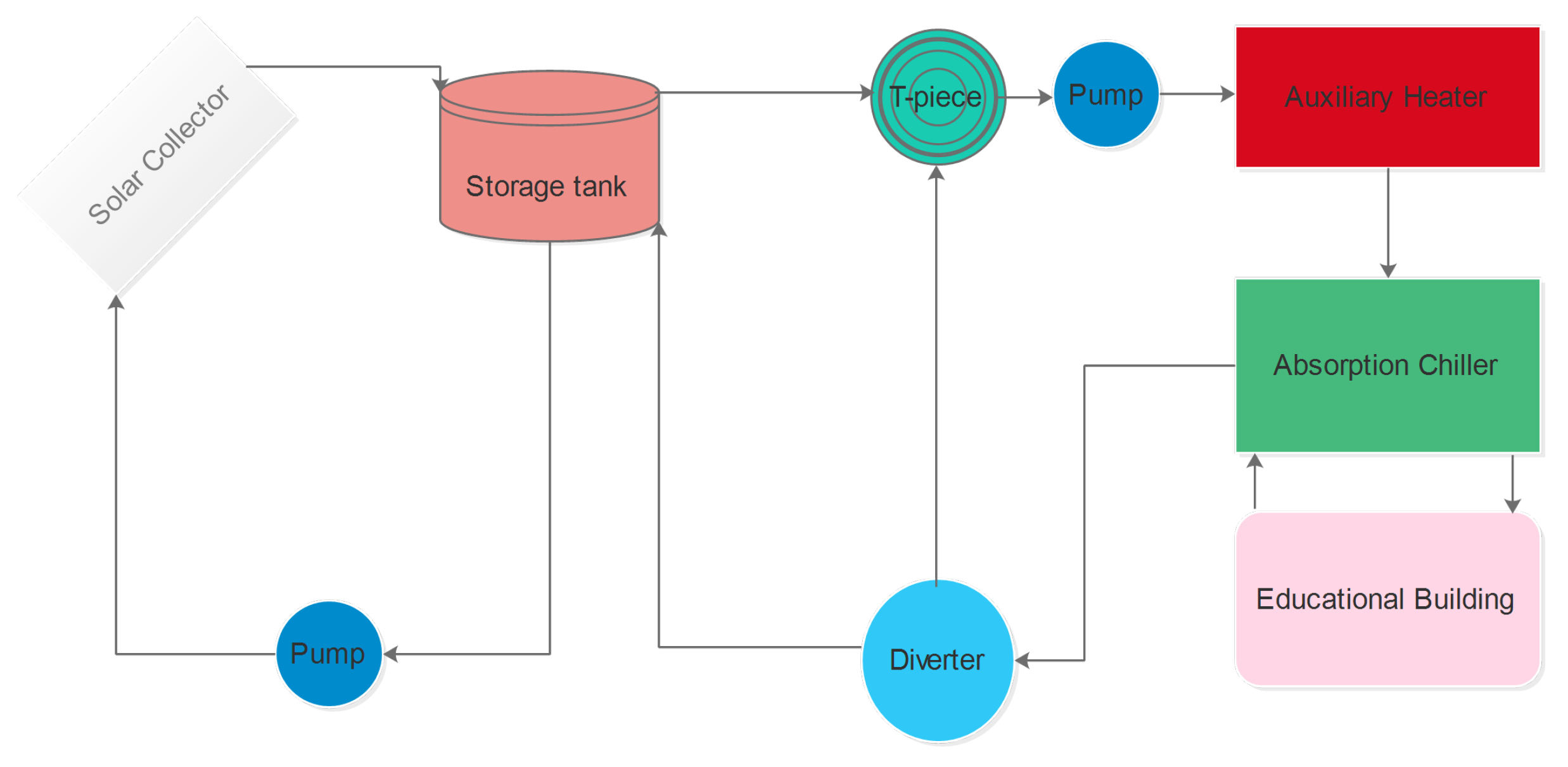
The schematic of the main components used in the solar absorption cooling system for educational building is shown in Figure 1. Heat transfer fluid (water in the current study) flows between different components of the cooling system to exchange its heat during flow. For analyzing the controlled flow of HTF, three loops are presented between the components of the cooling system in the current study i.e.,

• Collector–tank loop
• Storage–chiller loop
• Chiller–building loop

These loops of HTF are indicated by yellow, red and green colors respectively in Figure 2. The current study focused on the loop in which HTF feeding the generator of the chiller (i.e., storage–chiller loop). To the best of our knowledge, HTF can be circulated between the components of a storage–chiller loop by three different ways which are known as three proposed flow schemes of the current study.

In scheme 1, solar collector receives the radiations from the sun and and heat up the water that flows toward thermal storage which then circulates towards solar collector after increasing the temperature of stored hot water.

The flow of the collector pump is controlled in such a way that when the hot water inlet to the solar collector exceeds its outlet temperature, it will stop pumping. The minimum required input to the chiller unit is the 109 °C hot water (neglecting the boiling point as the system is pressurized) either at storage temperature (if it is equal to greater than 109 °C) or after heated by auxiliary unit fulfilling the requirement of refrigerant evaporation in the chiller’s generator and returns to the storage tank.

A pump is used to control the flow of hot water from the storage tank to the chiller only during the operating hours of the building. During this time period an auxiliary heating unit with the thermostat is used that turns on the pump when the temperature from the hotter side of the storage outlet is less than the required operating temperature to run the chiller.

In Figure 1, the removal of tee, diverter component and direct links (of storage to pump 2 and chiller to storage) in storage–chiller loop shows conventional flow pattern of heat transfer fluid which is named as scheme 1 of the current study.

In scheme 2, the conventional flow pattern is modified in such a way that when hot water ($T_{chiller,out}$) coming out from absorption chiller, it will divert towards the auxiliary heating unit instead of flowing directly towards the storage tank if storage’s outlet is colder compared to the water returning from chiller as shown in Figure 3a. A flow diverter was used for diversion of the chiller’s output hot water the to auxiliary heater and a tee piece component to pass the hot water either from storage tank or from diverter. The flow of water in the collector–tank and chiller–building loop is the same as in scheme 1 shown in Figure 2.

In scheme 3, the flow of heat transfer fluid is modified with one of the most advanced techniques by diverting the flow after coming out from the absorption chiller unit. Figure 3b illustrates the mechanism of scheme 3 in which hot water ($T_{chiller,out}$) will continuously divert towards the auxiliary heater unless the temperature of the storage tank’s hot side outlet would reach up to the minimum required temperature i.e., 109 °C for the chiller so that it will operate without consuming auxiliary energy. A controller signal has been introduced to generate the signal for diverter to start or stop the diversion of HTF, the remaining components are the same as scheme 2 as shown in Figure 2 with the only difference in the temperatures values for managing the diversion flow of chiller’s hot water outlet.

3. TRNSYS Modelling

TRNSYS is employed for the modeling and simulating all schemes of the heat transfer fluid flow between storage tank to the chiller in SACS. The monthly averaged solar radiations of hot climate cities of Pakistan (Lahore, Islamabad, Multan, Peshawar and Karachi) are compared as shown in Figure 4 and a cooling system in an educational building of Peshawar (highest radiations city of Pakistan) is chosen for modeling of the solar absorption cooling system, having 108 kW peak cooling load during the summer season and daily operating schedule from 9 a.m. to 5 p.m. TRNSYS model for modified flow schemes exhibited in Figure 2. Thick red lines shown in Figure 2 depict hot water loop from the storage to the chiller unit, yellow lines depict the collector–tank loop while green lines indicated loop of chilled water from the chiller to building. Scheme 2 and Scheme 3 are having the same components except for the temperature range for the diverter. Meteonorm weather data available with the TRNSYS v17 was used in the current model of SACS.

To accomplish the objective of comparing the performance of three proposed flow schemes of the study, the following assumptions are considered with the design of cooling system used:

• Heat losses from pipes are neglected.
• Energy balance technique is used for cooling tower specifications.
• Boiling effects of the heat transfer fluid are ignored.
• Electricity consumption of pumps is not included as the auxiliary energy consumption record.

Connections shown in Figure 2 are just logical connections and not represents pipes. For simplicity of the model, pipes or valves connections are not included in the current model by which heat losses from pipes can be measured as it can be assumed that they are perfectly insulated. The second assumption of the study reflects theoretical calculations of cooling water energy by energy balance equation i.e., Equation (6) which tells us energy from absorber and condenser rejected by cooling water by keeping the temperature difference of 5 °C between the inlet and outlet cooling water for design consideration in Equation (6) of the current study and no separate TRNSYS component of the cooling tower is used. The third assumption depicts the pressurized water system by which the normal boiling point of water can be varied, however, pressure calculations are not included in the study. All flow schemes of the current study use two flow pumps and would consume considerable but same amount of electricity as the designed flow rates are the same in all schemes, so that this electricity consumption of the pumps is not included as auxiliary energy consumption calculation.

With the aforementioned assumptions, it is suggested that this simulation study provides a somewhat higher evaluation of performance indicators than practically installed system but still, our sole purpose from this study of analyzing the effects on the performance of the solar cooling system due to modified flow schemes can be fulfilled with these assumptions.

3.1. Weather Data Processing

Weather data for the cities of Pakistan was taken from the built-in Meteonorm files provided with TRNSYS v17. Type 15-6 component used standard format data while Type 99 component used user format weather data file of Islamabad from Meteonorm Software because of the absence in TRNSYS v17 package.

3.2. Solar Thermal Collectors

An evacuated tube solar collector and a flat plate solar collector has been used in the current study to utilize solar energy for water heating. The second order incidence angle modifier efficiency equation [21] is described below:

$$\eta =a_0-a_1\frac{T_i-T_a}{I_T}-a_2\frac{{(T_i-T_a)}^2}{I_T}.$$

(1)

In Equation (1) $a_0$ is the intercept efficiency and $a_1$ and $a_2$ are the efficiency slope and efficiency curvature respectively. $I_T$ is the global solar radiations on the surface of the collector, $T_i$ is the temperature of the heat transfer fluid at collector inlet and $T_a$ is the temperature of ambient air. The mass flow rate of the Solar loop is set by considering the flow rate at the testing condition and area used. Technical data includes default values of Type1b for Flat plate collector from TRNSYS library and Evacuated tube collector (model number: Enertech Enersol HP 70-8). Further details of these collectors are provided in the

Table 1. Technical specifications of collectors.

Type of Controller	ETC	FPC
$a_0$	0.804	0.800
$a_1$ (kJ/h·m2·K)	1.56	13
$a_2$ (kJ/h·m2·K)	0.0054	40
Testing flow rate (kg/h·m2)	100	40
IAM longitudinal at 50°	0.93	$1-0.2(1/cos\theta -1)$
IAM Transversal at 50°	1	$1-0.2(1/cos\theta -1)$

.

3.3. Thermal Storage

Uninterrupted supply of solar energy input is provided by the use of thermal Storage tank of stratification type with all having 10 nodes and an energy balance approach is used to get the outlet temperature from each node over the prescribed time step [21]. The value of the designed flow rate from tank outlet to the chiller is given in

Table 2. Design parameters for solar absorption cooling system.

Designed Parameters	Values
Type 700 (Auxiliary Boiler)
Time step (minutes)	7.5
Boiler Efficiency (%)	85
Combustion Efficiency (%)	78
Type 107 (Single effect hot water fired Absorption Chiller)
Specific heat of heat transfer fluid (kJ/kg·K)	4.19
Chiller’s rate COP (default)	0.53
Hot water’s flow rate from tank to Chiller (kg/h)	17,507
Chilled Water’s flow rate from Chiller to Building (kg/h)	16,710
Cooling Water’s flow rate for condenser and absorber heat rejection (kg/h)	54,527
Minimum Temperature for chiller operation (°C)	109
Cooling water inlet temperature (°C)	29.4
Chiller Water Setpoint (°C)	6.667
Peak Cooling Demand (kW)	108
Auxiliary electrical energy for solution pumps etc. (KW)	5.55
Type 4a (Thermal Storage Tank)
Heat transfer coefficient for tank (W/m2·K)	0.83
Number of total nodes	10
Density of water stored in tank (kg/m3)	1000

. The losses from the tank are uniform and the value is 0.83 W/m² °C is considered. Hot water enters and exits from top sides and cold water replaces from bottom sides of the stratified tank as shown in Figure 5.

3.4. Auxiliary Unit

To raise the temperature of HTF up to 109 °C for generator operation of the chiller, a boiler is used as an auxiliary heating unit named type700 in TRNSYS library. This component gives the amount of energy consumed to raise the temperature of the water up to the desired temperature by considering input combustion and boiler efficiencies. When the heat transfer fluid enters the unit with a temperature less than the designed temperature, auxiliary heating unit turns on by the controller signal and heat up the fluid to the designed temperature. The boiler part load ratio is given by the following equation [21]:

$$PLR=\frac{Q_{need}}{Q_{max}}.$$

(2)

In this equation, $Q_{max}$ is the maximum capacity of the auxiliary unit and $Q_{need}$ is the amount of energy consumed by the auxiliary heating unit to keep the hot water temperature at the designed point. In order to raise the temperature of the incoming fluid, the value of $Q_{max}$ is selected in such a way that the part load ratio of the boiler should remain equal or less than one, for raising the temperature of incoming fluid.

3.5. Absorption Chiller

Single effect hot water fired absorption chiller (type107) is used to encounter the cooling load of the building. This component uses a catalog data lookup approach to predict the performance and gives the correct output by interpolation if given input are in the range of performance catalog file. In TRNSYS v17 catalog data file of type107, the operating range of inlet hot water temperature for the chiller’s generator is between 108 °C to 116 °C. Therefore, in current design, the minimum operating temperature of 109 °C is chosen to operate the absorption chiller to encounter the peak cooling load of 108 kW (31 TR). The inputs of this section is crucial for designing of the cooling system as the chiller’s capacity decides the amount of cooling demand that it can withstand. TRNSYS referenced formulation [21] is used for designing the parameters:

$$Q_{hw}=\frac{Capacit{y}_{rated}}{CO{P}_{rated}}{f}_{Designedenergyinput}.$$

(3)

In Equation (3), $Q_{hw}$ is hot water energy that must be available for the chiller operation, rated capacity and COP are given in Table 2 while $f_{Designedenergyinput}$ is taken from performance catalogue data file of type107 at designed conditions.

$$Q_{coolingcapacity}=m_{chw}C{p}_{chw}(T_{chw,in}-T_{chw,set}).$$

(4)

In Equation (4) $Q_{coolingcapacity}$ is the energy rate which must be removed by chiller (sometimes denoted by $Q_{remove}$ or $Q_{chilled}$) that must be removed by chiller, $m_{chw}$ is the flow rate of water from the chiller, $m_{chw}$ is flow rate of water out from the chiller, $C_{pchw}$ is the fluid’s heat capacity from the chiller and ($T_{chw,in}$−$T_{chw,set}$) is the difference between the temperature of the chilled fluid entering and leaving at the chiller which is taken by considering default values of inputs of type107 i.e., default values of $T_{chw,in}$ and $T_{chw,set}$ are 12.22 °C and 6.667 °C respectively, in current study.

$$Q_{hw}=m_{hw}C{p}_{hw}(T_{hw,in}-T_{hw,out}).$$

(5)

In Equation (5) $Q_{hw}$ is hot water energy that must be available for the chiller operation, $m_{hw}$ is the flow rate of hot water and is calculated from this equation by choosing the difference of hot water inlet and hot water outlet ($T_{hw,in}$−$T_{hw,out}$) value as 10 °C while $C_{phw}$ is the heat capacity of hot water. $Qcw$ is cooling water energy rate is found out by the energy balance approach in the current study i.e.,

$$Q_{cw}=Q_{chw}+Q_{hw}+Q_{aux}.$$

(6)

In Equation (6), $Q_{aux}$ is the auxiliary electricity consumed by the chiller for solution pumps and refrigerant pump etc. Equation (6) is used to balance the total energy of the chiller. This is the total energy rejected from chiller to environment and is used to find $Q_{cw}$. The $Q_{cw}$ will be further used in Equation (7) for design consideration. The design parameters are already tabulated in Table 2.

$$T_{cw,out}=T_{cw,in}+\frac{Q_{cw}}{m_{cw}{C}_{pcw}}.$$

(7)

where, $Q_{cw}$ is the energy required by the cooling water, $m_{cw}$ is the flow rate of cooling water and is found from the Equation (7) by fixing the temperature difference of cooling water outlet and cooling water inlet ($T_{cw,out}$−$T_{cw,in}$) as 5 °C while $C_{pcw}$ is the heat capacity of cooling water.

3.6. Hydronic Components

Type 114, Type 11h and Type 11f are the hydronic components as pump, tee-piece and the flow diverter respectively. These components are used for controlling the flow of heat transfer fluid with the aid of external control signals from the temperature controllers or conditional equations used in the model and with the designed mass flow rate. Flow diverter and tee-piece are used in flow schemes 2 and 3 where we need to divert the flow of hot water leaving the chiller, either towards the auxiliary or to the thermal storage by comparing the temperatures.

3.7. Controllers and Outputs

A five-stage thermostat component type108 for turning on the auxiliary heater and equations components for temperature comparison for stopping or starting the flow of the solar collector loop pump was used in all schemes. When the inlet temperature of the boiler is colder than the minimum required temperature of the chiller then the type108 causes the boiler to on, while the collector pump stops the flow by using the signal from the equation output value when inlet temperature exceeds the outlet temperature of the heat transfer fluid. Type65b, Type65c and Type25b are the output components used for obtaining output files in excel formats. Type14h is the forcing function that is used for generating a control signal at the input of the pump during the operating hours of educational building in this model.

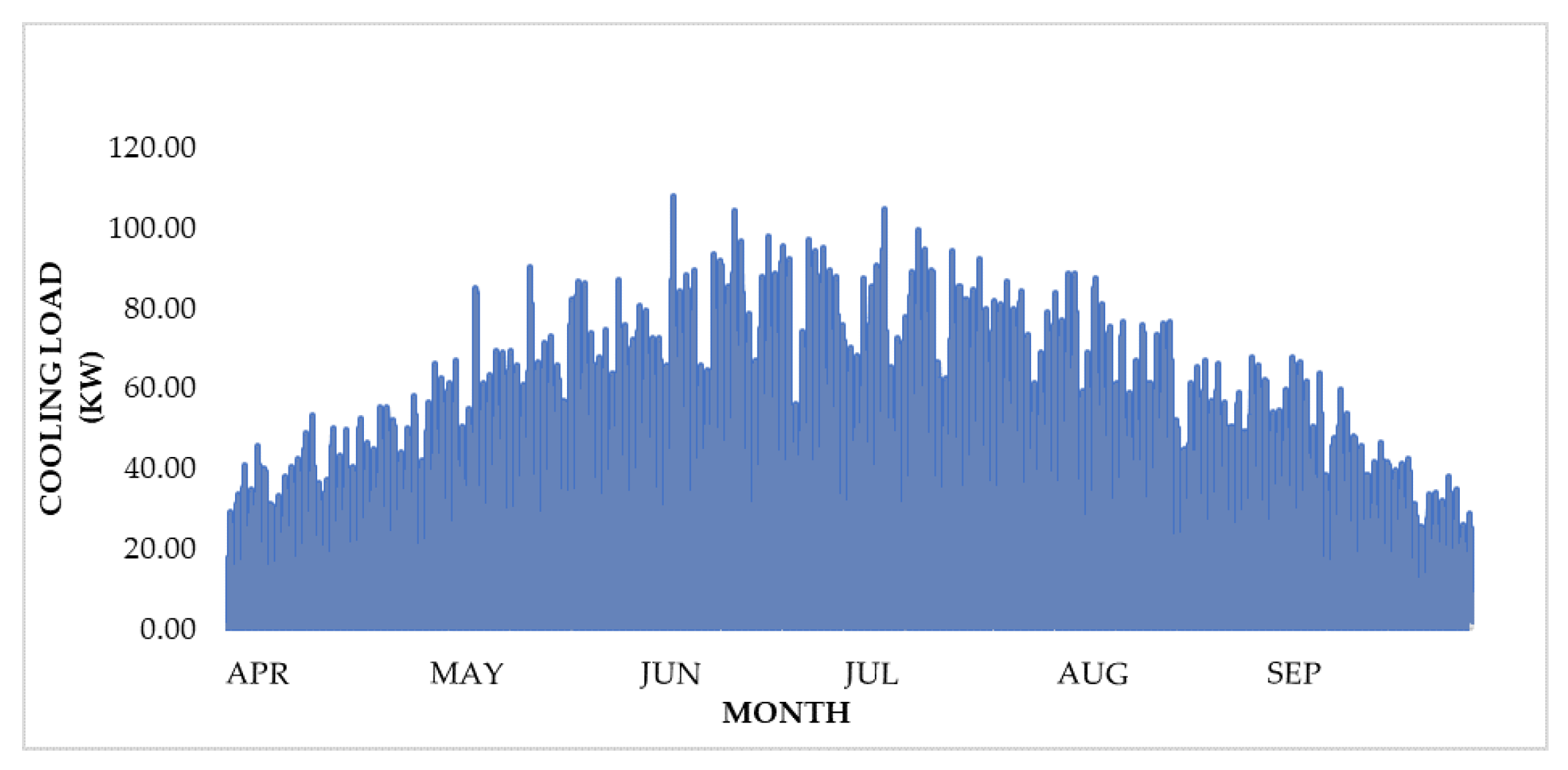
3.8. Building Load Generator

Type686 is the heating and cooling load generator component for the building synthetically. This component has been extensively used in previous studies [22,23,24] to save their time from tedious calculations. Type686 takes the input as peak load and gives hourly cooling load demand which is quite like real building load and also uses daily and seasonal variations in the load as shown in Figure 6. Type682 component takes its input of cooling load from type686 and inlet fluid’s temperature from the chiller’s output and returns water stream (i.e., chilled water inlet for chiller) after handling the cooling load of building.

4. Performance Indicators

Performance indicators for analyzing effects by comparing the performances of all schemes are given below:

4.1. Solar Fraction

Many studies used solar fraction as the main performance indicator in their study [3,4,5]. The solar fraction is defined [3] as:

$$SF=\frac{Q_{solar}}{Q_{solar}+Q_{boiler,aux}}.$$

(8)

where $Q_{solar}$ is the useful energy gain by the collector and $Q_{boiler,aux}$ is the auxiliary energy consumed by the boiler. Its value always remained between 0 and 1 having inverse relation as auxiliary energy consumed.

4.2. Primary Energy Saving

M. Shoaib et al. [11] used a generalized equation for fractional energy saving by which performance of the designed cooling system can compared with conventional VCCS for same cooling demand.

$$PES=1-\left[\frac{\frac{\int Q_{boiler,aux}}{{ϵ}_{heat}}}{\frac{\int Q_{cooling,ref}}{CO{P}_{ref}.{ϵ}_{elec}}}\right].$$

(9)

The numerators inside the square brackets represent the total auxiliary energy expenditure of the boiler in our system while the denominator represents the electrical energy consumed by the referenced conventional vapor compression system unit installed in the building. In the Equation (9), $\int Q_{boiler,aux}$ is the integrated value of auxiliary heat from boiler, ${ϵ}_{heat}$ is the efficiency of boiler having parametric value 0.78 in our system, $\int Q_{cooling,ref}$ is the integrated value of the energy for cooling effect realized from referenced conventional cooling system (i.e., 108 kW), COP value of the installed chiller (model number WCPS 380 BP R/H) installed in the building from the manufacturer is 3, while ${ϵ}_{elec}$ denotes the conventional efficiency of a thermal power plant (ratio of electrical energy generation to the primary energy consumption) whose value is considered as 0.4. The electricity consumption of the hydronic components is not considered in this study which may cause the investigated results to slightly deviate from the actual fraction of primary energy saving and saving of at least 50% primary energy is considered as worthwhile as economical point of view in this study.

5. Results and Discussion

TRNSYS model runs for the time span of summer months i.e., from April to September. As not enough exploratory information exists from a real framework, the current simulations are compared with the already published results for validation of the current model. M. Azmi and A.Q. Malik [25] found in their study that the best tilt angle plays an extensive role to expand the output of a solar collector. The determination of the optimum collector slope is influenced by using many limiting factors, such as deficiency of manpower body and inaccessibility of the region of solar collector subject due to which normal tuning of the slope is mostly not feasible. So, in our model, the greatest seasonal SF is acquired for the area at which 50% PES is achieved with an optimum collector slope of 9° for evacuated tube collector (ETC) and 15° for a flat plate collector (FPC) as shown in Figure 7.

Storage sizes are plotted for collector areas of FPC in Figure 8 at which flow schemes are realizing 50% seasonal primary energy savings. It is essential to note that the legends in Figure 8 and Figure 9 are representing the area of collector in m² used for one of the flow schemes of the study. For instance, legend 510 S1 means that 510 m² collector area used for flow scheme 1. Similarly, all other legends in Figure 8 and Figure 9 have same syntax.

It can be observed from Figure 8 that with increasing storage capacities, primary energy saving first increases, then start decreasing afterwards. For FPC, collector area of 635 m² with 30 m³ storage tank volume is required for achieving 50% PES with S-1 while collector area and storage tank volume is reduced to 550 m² and 20 m³ respectively, is used for saving 50% of primary energy.

In S-3, an optimized volume (10.2 m³) with a comparatively small collector area (than S-1 and S-2) is used to achieve the target of 50% primary energy saving. Similar trends are obtained for ETC as shown in Figure 9, however, the requirement of the collector area and storage tank size was greatly reduced because of the higher efficiency of the ETC [26]. With S-1, 128 m² collector area and 3 m³ storage tank, while S-2 simulated with reduced storage size of 2 m³ and 112 m² collector area to get 50% saving of the primary energy. A collector area of 93 m² was required to achieve 50% primary energy saving with scheme 3 of the current study with an optimum storage capacity of 15 L/m² (1.4 m³). The reason for decreasing PES with increasing storage sizes is that the higher tank sizes require more time to increase the tank’s average temperature so that more auxiliary energy will be consumed and for a longer span of time to heat up the colder intake of tank’s outlet. This is also the reason that S-2 would perform better than S-1 because S-2 diverts chiller’s outlet flow to the auxiliary unit when it is hotter than the tank’s outlet so that less auxiliary energy consumption as compared to S-1.

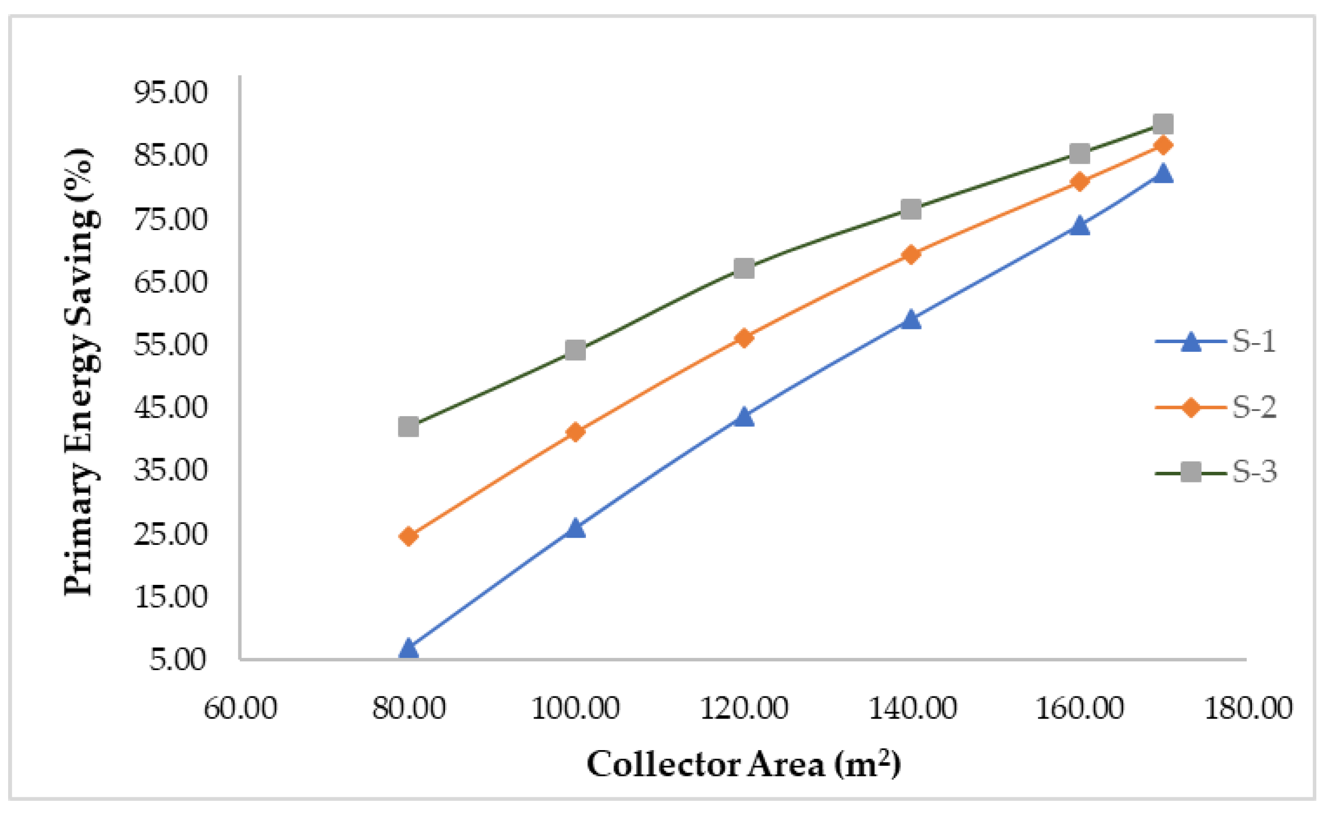
In Figure 10 and Figure 11, the seasonal variation of the fraction of energy-saving with collector areas of ETCs and FPCs to fulfil the cooling demand for all flow schemes is demonstrated at their optimum conditions. S-3 returns higher energy saving for ETC and FPC and S-1 yields less energy saving.

The trend in Figure 10 and Figure 11 is explained by Figure 12 and Figure 13, in which an area of 93 m² is selected with their optimum storage sizes and collector’s tilt of each scheme and simulated for the month of June. The results of a typical day of the summer season is plotted (3960–3984 h), in order to comprehend the fact that how schemes S1, S2 and S3 are acting in descending order of their primary energy-saving trend.

In Figure 12, it can be seen that auxiliary energy consumption of S-1 starts rising earlier in the day than S-2 and S-3 while auxiliary energy consumption of S-3 mostly fluctuates from zero to its maximum point many times a day. As is obvious from Equation (8), primary energy saving primarily depends on auxiliary energy consumption by the boiler in the system, so during operating hours of the building, the lowest (zero) value of S-3 auxiliary energy consumption (legend S3 aux cons) shown in Figure 12 gives a clear indication of the OFF condition of the boiler many times during the day and reflects higher PES than S-1 and S-2. 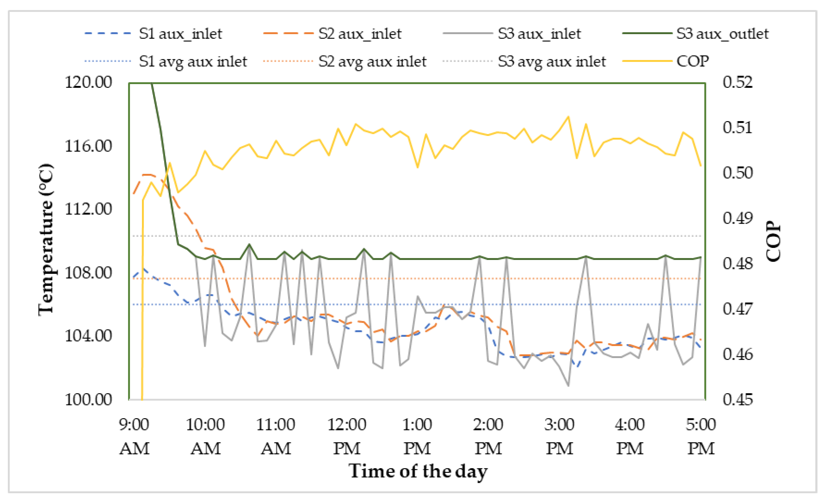However, in order to have a clearer and logical understanding that how boiler consumes energy to heat up the hot water up to the required temperature for chiller, Figure 13 explains the behavior of boiler and chiller component for all three schemes on operating hours of 15 June (i.e., 9 a.m. to 5 p.m). At the start of cooling operation, inlet temperature to the boiler was already higher than the minimum driving temperature of the chiller due to stored thermal energy in all three schemes. As time passes by, the hot water coming from the chiller combines and transfers heat with the water in the tank whose effect is to decrease the temperature of the fluid flowing towards the chiller and declining behavior of temperatures at the inlet of the auxiliary boiler was observed. Mechanism of modified flow schemes (S-2 and S-3) serves the purpose here for saving auxiliary energy by allowing the hot water to feed the boiler with higher temperatures than conventional scheme S-1. Figure 13 illustrates the transient behavior of inlet temperature to the boiler for all schemes throughout the operating hours of the day. It is also understood that the boiler’s outlet temperatures will be equal to the minimum required temperature of the chiller at the times when the boiler’s inlet is less than 109 °C for S-1 and S-2. COP for an optimized scheme is shown as the secondary axis of Figure 13. The dynamic profile of chiller’s generator outlet temperatures is displayed in Figure 14 with minor differences in their average values stayed under 103 °C. Dotted lines are the average temperatures for boiler inlet for the day in the month of June shown in Figure 13 is the clear and strong clue that why and how boiler consumes energy for heating up the hot water up to the minimum driving temperature (109°) for the chiller in descending order of S-1, S-2 and S-3.

In Figure 10, the probable reason for narrowing a gap between flow schemes curves (at higher collector areas) is that the boiler’s inlet HTF attains 109 °C so early and operates the chiller with higher generator inlet temperatures more than the minimum required temperature.

Returning fluid from chiller in case of S-2 and S-3 would remain above 109 °C for higher collector areas, so it does not matter if it is diverted or not because the inlet to the chiller will remain more than 109 °C that results in auxiliary unit remain in the OFF condition. The trend of primary energy saving with higher areas of FPC for all schemes is shown in Figure 11, where optimized flow scheme S-3 always performed better than the other two schemes.

Monthly efficiencies in Figure 15 are plotted at optimal thermal storage and collector slope and for the areas of ETC (93 m²) and FPC (510 m²) by which 50% primary energy saving would achieve by using flow scheme-3 of the current study i.e., monthly efficiencies of ETC are plotted for 93 m² area, the optimal thermal storage size of 15 L/m² and 9° collector tilt. Similarly, monthly efficiencies of FPC are plotted for 510 m², optimal storage size of 20 L/m² and collector tilt of 15°. In Figure 16 results of all proposed flow schemes of the study are summarized in term of collector area per kW of cooling.

6. Validation of Results

Monthly solar fraction curves obtained from three schemes of the current study as shown in Figure 17a was compared with a study by Assilzadeh et al. [7], shown in Figure 17b and we found similarity of the trends for the months of summer season. It can be seen from Figure 17b that the solar fraction is plotted for entire year in previous published article while in current study, results of solar fraction from April to September were evaluated for the parameters of 50% PES and plotted in Figure 17a. Legends (10 to 100) in the already published paper representing different collector areas used. Lower solar fractions at the mid of the season (July) is an indication of higher auxiliary energy consumption and lowest primary energy saving month of the season justifying Equations (8) and (9) of the current study.

Tilt angles of the collector of S-3, using optimum storage size, were plotted against seasonal collector gain obtained for ETC in the current study. As Figure 18a,b exhibited a fairly similar trend for the optimum tilt angle of the collector. Figure 18a matching with Assilzadeh et al. [7]. However, the optimum value of the tilt angle of the solar collector depends upon the specific location, therefore, plots may differ in values (because of different collector areas used) and units, but trends are found to follow similar paths in both current and previous studies).

Another similarity of the trend for storage size with auxiliary energy consumption for cooling system is shown in Figure 19, as minimum value of auxiliary energy consumption corresponds to the optimum tank volume. It can be clearly seen that the current study (Figure 19a) is quite similar to the Djelloul et al. [27] study shown in Figure 19b for relation between storage size and auxiliary energy.

7. Conclusions

Solar absorption cooling system designed for a peak cooling demand of 108 kW was modeled and simulated by using TRNSYS. The components in the TRNSYS standard library are employed and linked in all possible flow schemes between the storage–chiller loop with different control strategies of the working fluid. An educational building located at Peshawar (34° N, 71.54° E), where a vapor compression cooling system of 108 kW cooling capacity was replaced by SACS, was selected to simulate the system for the whole summertime. The best collector slope was found to be around 9° for ETC and 15° for FPC at the highest solar fraction. Results also indicated a perceptible difference between maximum monthly averaged efficiencies for both collector types as shown in Figure 13. Hence, it can be decided that the flat plate collector is not an ideal option for the presented study because of the requirement of more than five times larger area than ETC. Primary energy saving is much better for Scheme 3 compared to Schemes 1 and 2 with matching storage at somewhat smaller collector areas for ETC. The discrepancy in the fraction of primary energy saving of all schemes shrinkages for higher collector area as shown in Figure 9 and Figure 10, but for real scenarios, economics consideration of the system is also involved while deciding to use higher collector areas. Monthly SF curves for ETC, as shown in Figure 15, in current simulation results also indicated S-3 is far better than the other two schemes to be exploited. In Figure 16, collector area per kW of refrigeration is plotted. Scheme 3 has the smallest area/kW for both ETC and FPC for achieving 50% energy savings. Overall, flow scheme-3 with evacuated tube collector is considered as the best selection for the current study to use with the smallest ratio of collector area to kW of cooling capacity. Because of insufficient experimental records that can be used for direct validation of current results, trends in previous publications of simulation studies were found to be matched with current simulation trends.