Methods to Apply a 3-Parameter Logistic Model to Wind Turbine Data

Abstract

Power curves provided by wind turbine manufacturers are obtained under certain conditions that are different from those of real life operation and, therefore, they actually do not describe the behavior of these machines in wind farms. In those cases where one year of data is available, a logistic function may be fitted and used as an accurate model for such curves, with the advantage that it describes the power curve by means of a very simple mathematical expression. Building such a curve from data can be achieved by different methods, such as using mean values or, alternatively, all the possible values for given intervals. However, when using the mean values, some information is missing and when using all the values the model obtained can be wrong. In this paper, some methods are proposed and applied to real data for comparison purposes. Among them, the one that combines data clustering and simulation is recommended in order to avoid some errors made by the other methods. Besides, a data filtering recommendation and two different assessment procedures for the error provided by the model are proposed.

1. Introduction

Wind turbine performance is usually described by means of the relationship between output power and wind speed. The manufacturers provide these curves, or alternatively a set of points representing pairs of wind speeds and powers, after testing the wind turbine according to the IEC (International Electrotechnical Commission) Standard procedure (IEC 61400-12) [1]. The process to obtain such curves is based on the definition of bins of 0.5 m/s, from where pairs of data are taken (wind speed, output power). The Standard states that at least 180 minutes of total data must be taken and, also, at least 30 minutes of data per bin must be included in the test. Besides, turbulence is a very important circumstance to be taken into account when obtaining the power curve because the output power of a wind turbine is also influenced by it. Moreover, some specific corrections must be included in the test in order to reach the proper power curve as explained in [2,3]. These corrections are not considered in this research and may be considered as a future work.

The information described in the previous paragraph is enough to analyze the behavior of a wind turbine under normal operating conditions and the results provided can be considered valid when estimating or assessing its performance in an aggregate way. However, in the case of installed wind turbines, the working conditions may be very different from the expected ones: weather [4,5,6], terrain conditions [7,8,9] and aging [10,11,12,13] may affect their performance. In the latter case, only real data can provide an accurate information of the wind turbine behavior.

In a real case, discarding wrong or out of range data is critical. Errors in the measurement process or even in the wind turbine performance cannot be considered when trying to model or simulate its real behavior. Therefore, real data filtering before analysis is needed [14,15,16].

Filtered data can be analyzed in order to model or simulate wind turbine behavior [17]. As there is a wide variability in the real data [18], and the objective is to have accurate information of the installed wind turbine, a possible option is to use the simplest model for the power curve with valid results. Linear [19], quadratic [20] and cubic [21] models are discarded due to their inaccuracy. Splines [22] are very complex due to the high number of parameters and the lack of a unique expression due to the piecewise definition. Another option might be to use the sigmoid functions (‘S’ shape functions) that combine a low number of parameters with a single expression which makes them suitable to be implemented in direct calculations and in compounded expressions. Among them, the logistic-type functions have been successful in wind power curve modeling.

Logistic functions were introduced as models of population growth and nowadays are used in statistics, medicine, linguistics, agriculture, economics or sociology [23,24,25,26]. Lately, they were introduced to model wind turbine power curves with success due to their simplicity, diversity and versatility. Among them, the so called 3PLE (Three parameter logistic exponential) was chosen as the most suitable one because it only needs three parameters and its error level is very low [27,28].

In spite of all the above, there is not just a single way to apply a specific model to wind turbine data analysis. From the filtered data to the model itself there are several options to proceed. The simplest method to apply the model may be to define a number of intervals for the wind speed, to identify each interval by the mean value and to assign the mean output power as the corresponding value for each wind speed identifier. With these pairs of values, i.e., points in a graph, the model can be defined as the function that best represents the points, by using an optimization process for an objective function which is the error made [29,30,31]. An optimization process is based on an algorithm and, in this paper, the Interior Point Algorithm has been chosen because it is well known due to its satisfactory performance when dealing with a wide variety of problems. There are some other methods to apply the model, such as using all the existing data, defining a different objective function, etc. When comparing the methods to apply the model, the error made when using the different models constitutes a proper metric for assessing their performances.

This paper is organized as follows: the process of filtering data is depicted in Section 2, the description of the methods applied is shown in Section 3, assessment errors are defined in Section 4, the case study is shown in Section 5 and the conclusions are outlined in Section 6.

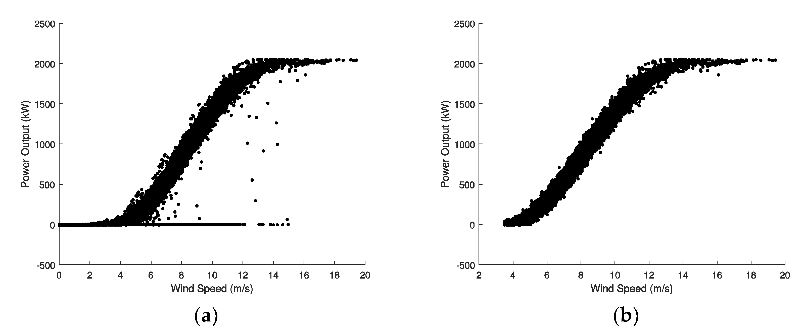
2. Data Filtering

In order to apply the methods proposed in this work in a proper manner, only valid data need to be considered, which means that raw data have to be filtered. From the point of view of the values, wrong data can be classified into two groups: those values that are clearly outside the proper range and those values that are close to being valid but must be discarded, too. For the first ones, the following procedure was applied:

• To discard wind speed values that are lower than the cut-in wind speed.
• To discard wind speed values that are 1.5 m/s above the cut-in wind speed, when they provide an output power lower than a 5% of the rated power.
• To discard wind speed values that are 1 m/s above the rated wind speed, when they provide an output power lower than a 75% of the rated power.

The limits correspond to values clearly out of bounds, i.e., clearly dispersed and out of place in the data cloud. In the second case, and in order to establish a reasonable limit, a filter based in a Normal distribution is applied. In this case, the mean power (µ) is obtained for all the wind speed values that correspond to an interval of 0.5 m/s and, centering a Normal distribution in those values, all the values outside the range µ ± 3σ are discarded, being σ the standard deviation of the values in that interval. As a final checking, if the percentage of values discarded is over 5%, those limits have to be reconsidered.

In Figure 1, raw data and filtered data are shown in order to be compared.

3. Methods Proposed

In order to define the best method to assess the application of the model to the wind turbine power curve, firstly the reference one is defined, based on the spline, by using the same procedure as the one proposed by IEC 61400-12. Notice that the curve obtained is not the same as the one provided by the manufacturer because, for the latter case, the conditions to perform the test are standardized. Then, the rest of methods are depicted: Clustering, Cloud data, Cluster simulation and Maximum error cluster. The input data in all cases is the filtered data.

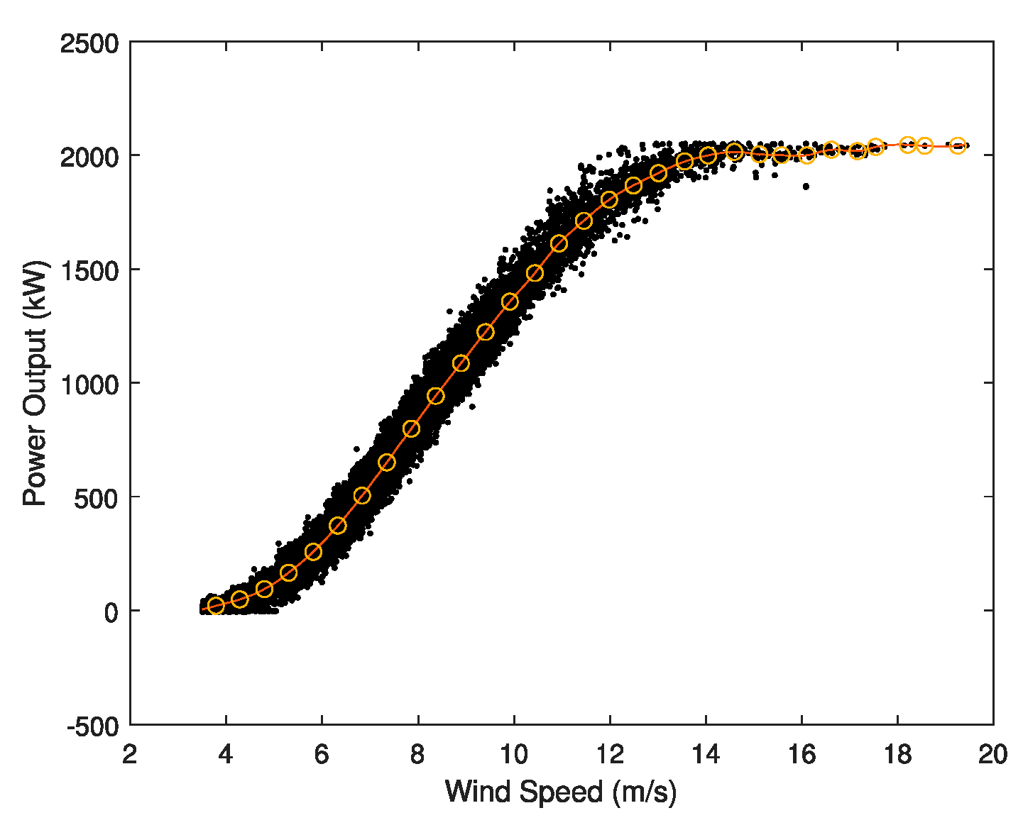
3.1. Spline

The reference case is based on the spline model. It uses the mean values on each interval (i.e. 0.5 m/s) to be the points of continuity of 3-degree polynomials. In those points, the derivation of the function are satisfied. The reference is considered because wind turbine manufacturers provide a number of pairs of points, and those pairs of values do not allow to obtain a better approximation than the spline. Its cons are the high number of parameters involved (four every 0.5 m/s) and the difficult combination of the function with others (i.e. the wind speed Probabilistic Density Function).

The procedure to obtain the spline by means of filtered data is the following:

• Divide the data into intervals, one every 0.5 m/s. The identification of each interval is an integer or the mean value of two consecutive integers. Notice that the number of data on each interval may be different.
• Obtain the mean power on each interval and assign that value to the identification of the interval on each one, too. The result is a number of pairs of values (wind speed, output power).
• Finally, the spline according to Equation (1) is obtained. Using MATLAB (R2019a, Mathworks Inc.), all the points for the spline are provided.

$$P\left(v\right)=a_i{v}^3+b_i{v}^2+c_{i}v+d_i\hspace{1em}\forall i\in \left[1:50\right]$$

(1)

where $a_i, b_i, c_i, d_i$ are the corresponding parameters for the wind speed ($v$) belonging to interval $i$. The spline, the points used to obtain it and the filtered data can be seen in Figure 2.

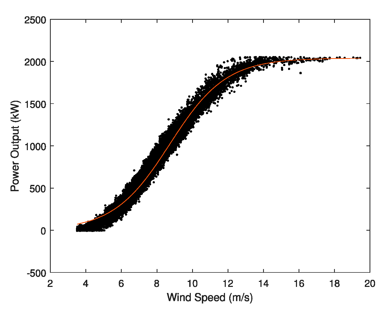
3.2. Clustering

The first method for applying the model is based on clustering, i.e., intervals of 0.5 m/s are defined and, in each one, a mean value for the output power is obtained. In every case, the mean output power is assigned to the identifier of the interval and, as a final result, pairs of values are obtained. After this, an optimization process is performed considering a specific model. In this paper, 3PLE one is used but the procedure is valid for any other. The 3PLE model follows the expression given by Equation (2), where α, β and γ are the only parameters. In order to a better fitting of the model, only pairs of values greater than the cut-in wind speed ones are considered.

$$P\left(v\right)=\frac{\alpha }{1+\exp \left(-\beta \ast \left(v-\gamma \right)\right)}$$

(2)

The optimization is performed by using the above mentioned Interior Point Algorithm and the results are the values of the parameters that best approximate the pairs of values. The optimization process has, as its objective function, the Least Squares Error, due to its performance in this type of algorithms.

The Interior Point Algorithm solves optimization problems by going through the middle of the solid defined by the problem rather than around its surface. The possible solution evolves on each iteration inside the feasible set to search the optima and it is stopped when the solution obtained cannot be optimized any more by the algorithm.

The algorithm is applied using the “optimtools” package provided by MATLAB, where some maxima and minima for the parameters need to be defined in order to accelerate the process. The application of the model based on clustering is shown in Figure 3.

3.3. Cloud Data

Another way to apply the model to filtered data consists of optimizing it with respect to all the data (cloud data), instead of only the mean values. Besides, the data are not divided, or clustered, into intervals. On the contrary, all of them have the same influence in the model obtained. In this case, the 3PLE model is used again and parameters α, β and γ of Equation (2) are obtained by optimizing that expression through the Interior Point Algorithm, and by using the Least Squares Error, as in the previous case. Therefore, in this case, the parameters of the 3PLE model are obtained by using all the filtered data through the Interior Point Algorithm. The model using this method can be seen in Figure 4.

It can be clearly seen that the curve obtained is far from expected for wind speeds higher that the rated wind speed, where there are not so many data available. The reason is that, using an optimization process, the result provided is good from a numerical point of view (the total sum of errors is not very high, even though a few of them are quite high) but very bad from the modeling point of view.

3.4. Cluster Simulation

The procedure, in this case, is a hybridization of the two previous methods. On one hand, using the filtered data, a better way to optimize the model than using the means is provided. On the other, clustering is needed in order to provide the same importance to all data, avoiding errors due to intervals with a low number of data.

Therefore, the process in this case is as follows:

• Divide the data in intervals, one every 0.5 m/s. The identification of each interval is an integer or and the mean value of two consecutive integers. This method is just an alternative when the number of data on each interval is different, as usual.
• Obtain the mean power and the standard deviation for each interval.
• Afterwards, a Normal distribution of the data on each interval is assumed and, with the parameters (µ, σ) obtained, values of power for each interval are simulated. The number of values generated for each interval has to be the same and has to be representative of all the possibilities (i.e. 200) The simulation has to be performed using MATLAB.
• Using the simulated values as data, the process depicted in the method Cloud data is applied.

The result of the application of the model using this procedure is shown in Figure 5.

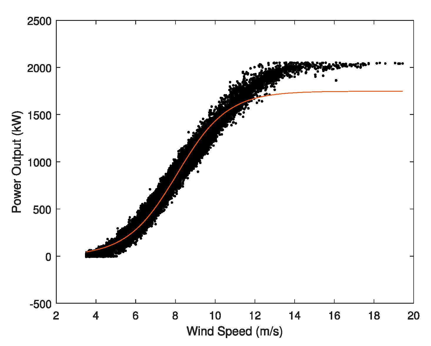
3.5. Maximum Error Cluster

The last method proposed with the aim of applying a model to the wind turbine power curve is based on a different focus. In the described methods, the optimization is based on a given objective function. In this case, a new error is defined according to equation instead of using the Least Squares Error (3). The reason is that the Least Squares Error is a sum of errors and, instead of optimizing the sum of errors, the maximum mean error on each interval can be a better objective to optimize.

The procedure is the same as in the method “Cloud data” but the objective function used in the Interior Point Algorithm is the maximum of the expression in Equation (3).

$${\overline{e}}_i=\frac{{\displaystyle \sum }abs\left(Pmode{l}_j-Pdat{a}_j\right)}{n_i}$$

(3)

Therefore, the objective function is $max\left({\overline{e}}_i\right)$. The application of the model using this method can be seen in Figure 6.

4. Method Assessment

In order to assess the performance of the described methods, a suitable criterion must be defined. Two measurements of the error committed are taken into account. Therefore, the lower they are, the better the performance of the method is. Both measurements take the Mean Absolute Percentage Error (MAPE) as a reference. They are the following:

• Cloud Data MAPE: it measures the difference, in absolute value, between the value provided by the model and the output power value (from the filtered data). It is obtained according to Equation (4).

  $$Cloud Data MAPE=\frac{{\displaystyle \sum }abs(Pmode{l}_j-Pdat{a}_j)}{Prated}$$

  (4)
• Mean Values MAPE: it measures the difference, in absolute value, between the value provided by the model and the corresponding mean value of the power. In order to obtain the mean values, intervals of 0.5 m/s were taken. It is obtained according to Equation (5).

  $$Mean Values MAPE=\frac{{\displaystyle \sum }abs(Pmode{l}_j-Pmea{n}_j)}{Prated}$$

  (5)

5. Case Study

In order to check the performance of the methods, real data measured at the wind farm of Le Haute Borne (Meuse, France) along five years (2013–2017) were used. The data were downloaded from the French company Engie web page, https://opendata-renewables.engie.com/, updated on 9 October 2019. In that link data from four wind turbines of the wind farm were available. Each provided measurement that corresponds to the 10-minute mean value of each variable. Besides, the data were analyzed by year and by wind turbine in order to reduce possible errors and to improve the models obtained. This means that each wind turbine of the same type may have slight differences on its performance and, from one year to the following, aging may reduce the power supplied. The features of the wind turbines used by Engie in the wind farm of Le Haute Borne are described in

Table 1. Wind turbine features in Le Haute Borne wind farm.

Manufacturer	Model	Rated Power (kW)	Hub Height (m)	Rotor Diameter (m)	Rated Wind Speed (m/s)	Cut-in Wind Speed (m/s)	Cut-out Wind Speed (m/s)
Senvion	MM82	2050	80	82	14.5	3.5	25

.

As it was described above, first, raw data were filtered and, then, all the methods were applied for the 3PLE model. Finally, the methods were assessed by using the two measurements of errors described in the previous section, i.e., Cloud data MAPE (CD MAPE) and Mean values MAPE (MV MAPE). The results of the performance are given in

Table 2. Performance of wind turbine R80711 for different methods.

	2013	2014	2015	2016	2017
CD MAPE spline (%)	1.71	1.64	2.14	1.94	2.08
MV MAPE spline (%)	0.00	0.00	0.00	0.00	0.00
CD MAPE clustering (%)	2.62	2.60	3.27	3.17	3.23
MV MAPE clustering (%)	1.16	1.40	1.29	1.38	1.81
CD MAPE cloud data (%)	2.26	2.11	2.77	2.57	2.66
MV MAPE cloud data (%)	6.86	6.34	5.87	7.07	6.94
CD MAPE cluster simulation (%)	2.57	2.53	3.15	3.05	3.23
MV MAPE cluster simulation (%)	1.21	1.39	1.34	1.44	2.02
CD MAPE max error cluster (%)	2.70	2.68	3.20	3.13	4.71
MV MAPE max error cluster (%)	1.76	1.62	2.24	2.52	4.63

,

Table 3. Performance of wind turbine R80721 for different methods.

	2013	2014	2015	2016	2017
CD MAPE spline (%)	1.50	1.30	1.79	1.68	1.76
MV MAPE spline (%)	0.00	0.00	0.00	0.00	0.00
CD MAPE clustering (%)	2.61	2.49	2.99	2.95	2.81
MV MAPE clustering (%)	1.25	1.36	1.52	1.35	1.46
CD MAPE cloud data (%)	2.01	1.73	2.34	2.24	2.33
MV MAPE cloud data (%)	8.85	8.60	6.91	7.77	6.81
CD MAPE cluster simulation (%)	2.51	2.41	2.91	2.79	2.69
MV MAPE cluster simulation (%)	1.30	1.42	1.54	1.43	1.48
CD MAPE max error cluster (%)	2.66	2.52	3.29	3.11	2.65
MV MAPE max error cluster (%)	1.60	1.59	1.53	1.55	2.05

,

Table 4. Performance of wind turbine R80736 for different methods.

	2013	2014	2015	2016	2017
CD MAPE spline (%)	1.50	1.42	1.76	1.64	1.75
MV MAPE spline (%)	0.00	0.00	0.00	0.00	0.00
CD MAPE clustering (%)	2.42	2.42	2.80	2.82	2.78
MV MAPE clustering (%)	1.11	1.26	1.27	1.18	1.18
CD MAPE cloud data (%)	2.03	1.89	2.35	2.22	2.35
MV MAPE cloud data (%)	6.57	5.99	5.09	6.33	6.11
CD MAPE cluster simulation (%)	2.31	2.30	2.69	2.64	2.70
MV MAPE cluster simulation (%)	1.14	1.32	1.29	1.24	1.19
CD MAPE max error cluster (%)	2.54	2.68	3.51	2.89	3.04
MV MAPE max error cluster (%)	1.41	1.28	1.46	1.64	2.19

and

Table 5. Performance of wind turbine R80790 for different methods.

	2013	2014	2015	2016	2017
CD MAPE spline (%)	2.04	1.62	2.33	2.16	2.27
MV MAPE spline (%)	0.00	0.00	0.00	0.00	0.00
CD MAPE clustering (%)	4.69	2.85	3.62	3.49	3.50
MV MAPE clustering (%)	1.60	1.51	1.52	1.40	1.27
CD MAPE cloud data (%)	3.48	2.14	3.00	2.83	2.96
MV MAPE cloud data (%)	11.45	6.88	6.36	7.08	7.37
CD MAPE cluster simulation (%)	4.93	2.78	3.42	3.33	3.39
MV MAPE cluster simulation (%)	1.50	1.53	1.58	1.47	1.29
CD MAPE max error cluster (%)	3.84	2.83	4.06	4.15	3.71
MV MAPE max error cluster (%)	3.97	2.04	1.86	3.30	2.96

, where each table corresponds to a different wind turbine. On each one, columns mean a different year and rows a specific combination of method and measurement of error. Notice that including turbulence corrections when applying these methods will be very valuable, however it has been discarded for simplicity.

CD means Cloud Data, MV refers to Mean Value and MAPE is the acronym of Mean Absolut Percentage Error.

In the first wind turbine, the analysis of the errors obtained by each combination of method and type of error provides the following items to be pointed out:

• In the reference case the MV MAPE is always 0 because it is the definition of the reference. However, when obtaining the CD MAPE, the value obtained is close to 2%. The reason is that all the pairs of points do not correspond exactly with the spline models, there is some variability.
• In all cases, the MV MAPE is lower than the CD MAPE because the latter measures the errors of all the pairs of points with respect to the model, so the variability is higher. There is an exception to the previous rule and is in the case of the cloud data because, in that case, all the pairs of points participate with the same weight in the model.
• The errors provided by the Clustering and the Cluster simulation methods are very low in both cases. In fact, in both cases the difference between the CD MAPE and the MV MAPE is lower than the corresponding one of the spline.
• Comparing Clustering and Cluster simulation methods, they provide very similar results in this case.
• In the case of the Max error cluster method, the values of errors are a bit higher in all cases.

Analyzing the second wind turbine, a similar discussion can be made and the following comments can be added:

• The CD MAPE for the Spline is a bit lower than in the case of the first wind turbine. The reason may be that the variability of the output power of that wind turbine is lower than in the first one which can be due to performance reasons.
• The MV MAPE Cloud data is higher than in the first wind turbine while the CD Cloud data is lower. The reason may be the same as in the first comment, the pairs of points are not very dispersed, therefore, they provide a very good model, when assessing all data.

For the third wind turbine, the following comments can be made:

• It is the wind turbine with the lower errors from a general point of view. The MV MAPE Clustering and the MV MAPE Cluster simulation errors are close to 1%.
• Its behavior and levels of errors are very similar to the ones of the first one.

In the fourth wind turbine some differences can be pointed out with respect to former wind turbines:

• The CD MAPE for the spline is over 2% (very high compared with the others).
• The CD MAPE Clustering is also very high (more than 3%).
• The MV MAPE for Clustering and Cluster simulation are very similar to the rest of wind turbines.
• The rest of errors are out of the ranges of the other three wind turbines.

In

Table 6. Comparison of the mean performance of the methods.

Optimization Method	Cloud Data MAPE (%)	Mean Values MAPE (%)
Spline	1.80	0.00
Clustering	3.01	1.36
Cloud data	2.41	7.06
Cluster simulation	2.92	1.41
Maximum error of cluster	3.19	2.16

, the mean values of the error measurements are provided organized by method and by type of measurement in order to assess the performance of each method on its own.

The Cloud data is the one that provides a lower percentage of error when it is measured using the CD MAPE. However, when considering the MV MAPE, the error obtained is far from the expected (7.06%). The reason may be that the data are dispersed.

Besides, the method based on the maximum error of the clusters is not a good option due to the results provided in both cases, the worst in the CD MAPE (3.19%) and the next to the worst in the MV MAPE (2.16%).

Also, influence of aging can be assessed and compared for the proposed methods. In general, it can be said that there is no specific influence but the slight increment of the error values with the aging for all the methods.

Finally, both methods based on clustering provide good results and, after discarding the others, the results obtained are the best when assessing the CD MAPE (Clustering simulation) and the MV MAPE (Clustering).

6. Conclusions

The power generated by a wind turbine can be different from that predicted by the manufacturer’s power curve due to several reasons such as aging, difference between test conditions and real-life ones, or even performance efficiency. A full year of data measurement may be enough to ensure a good assessment of its current performance, but even in this case good practice recommends data filtering and modeling. The models with low number of parameters, such as the 3PLE, which is a logistic model, are very useful to obtain instantaneous values and to be combined with other expressions (i.e. wind speed Probability Density Function). In order to obtain the parameters of the model that better fits the data, several methods can be applied. However, some methods have performance errors due to the difference in the number of data available on each interval of the power curve. In this paper, two methods to face this problem are proposed: Clustering and Cluster simulation. In both cases, the optimization is based on intervals and provide better results than those obtained by means of other methods. The second one is specially recommended when there is a low number of available data in some intervals because it can reproduce the behavior of the wind turbine, in order to balance the number of data. Besides, in the case of the IEC 61400-12, the application of the Cluster simulation method can provide better results than just using the data obtained. This means that, for the highest bins, the information may not be enough to properly define some parts of the curve.

Therefore, the method based on Cluster simulation can be used to obtain the best power curve when there are not so much data available in some of the bins. On the other hand, in the general case the method based on Cluster can be used for the same purpose. Both methods provide acceptable error values when applied to the 3PLE model, i.e., to a model of just three parameters, which outperforms the spline model, which needs around two hundred. The model obtained can be combined with a wind speed distribution to provide an output power distribution that can be the input for solving the Probabilistic Load Flow problem in an electrical network with wind power.

References

- IEC 61400-12-1:2017. Wind Energy Generation Systems- Part 12-1: Power Performance Measurements of Electricity Producing Wind Turbines; International Electrotechnical Commission: Geneva, Switzerland, 2017.
- Kaiser, K.; Langreder, W.; Hohlen, H.; Højstrup, J. Turbulence Correction for Power Curves; Peinke, J., Schaumann, P., Barth, S., Eds.; Springer: Berlin/Heidelberg, Germany, 2007. [Google Scholar]
- Möllerström, E.; Ottermo, F.; Goude, A.; Eriksson, S.; Hylander, J.; Bernhoff, H. Turbulence influence on wind energy extraction for a medium size vertical axis wind turbine. Wind Energy 2016, 19, 1963–1973. [Google Scholar] [CrossRef]
- Davis, N.N.; Pinson, P.; Hahmann, A.N.; Clausen, N.-E.; Žagar, M. Identifying and characterizing the impact of turbine icing on wind farm power generation. Wind Energy 2016, 19, 1503–1518. [Google Scholar] [CrossRef]
- Hoolohan, V.; Tomlin, A.S.; Cockerill, T. Improved near surface wind speed predictions using Gaussian process regression combined with numerical weather predictions and observed meteorological data. Renew. Energy 2018, 126, 1043–1054. [Google Scholar] [CrossRef]
- Paiva, L.T.; Veiga Rodrigues, C.; Palma, J.M.L.M. Determining wind turbine power curves based on operating conditions. Wind Energy 2014, 17, 1563–1575. [Google Scholar] [CrossRef]
- Dai, J.; Tan, Y.; Shen, X. Investigation of energy output in mountain wind farm using multiple-units SCADA data. Appl. Energy 2019, 239, 225–238. [Google Scholar] [CrossRef]
- Han, X.; Liu, D.; Xu, C.; Shen, W.Z. Atmospheric stability and topography effects on wind turbine performance and wake properties in complex terrain. Renew. Energy 2018, 126, 640–651. [Google Scholar] [CrossRef]
- Vahidzadeh, M.; Markfort, C.D. Modified power curves for prediction of power output of wind farms. Energies 2019, 12, 1805. [Google Scholar] [CrossRef]
- Dai, J.; Yang, W.; Cao, J.; Liu, D.; Long, X. Ageing assessment of a wind turbine over time by interpreting wind farm SCADA data. Renew. Energy 2018, 116, 199–208. [Google Scholar] [CrossRef]
- Li, J.; Li, Q.; Zhu, J. Health condition assessment of wind turbine generators based on supervisory control and data acquisition data. IET Renew. Power Gener. 2019, 13, 1343–1350. [Google Scholar] [CrossRef]
- Staffell, I.; Green, R. How does wind farm performance decline with age? Renew. Energy 2014, 66, 775–786. [Google Scholar] [CrossRef]
- Choi, H.S.; Yu, H.; Lee, E.Y.; Loza, B.; Pacheco-Chérrez, J.; Cárdenas, D.; Minchala, L.I.; Probst, O. Comparative fatigue life assessment of wind turbine blades operating with different regulation schemes. Appl. Sci. 2019, 9, 4632. [Google Scholar]
- Sainz, E.; Llombart, A.; Guerrero, J.J. Robust filtering for the characterization of wind turbines: Improving its operation and maintenance. Energy Convers. Manag. 2009, 50, 2136–2147. [Google Scholar] [CrossRef]
- Wang, Y.; Hu, Q.; Li, L.; Foley, A.M.; Srinivasan, D. Approaches to wind power curve modeling: A review and discussion. Renew. Sustain. Energy Rev. 2019, 116, 109422. [Google Scholar] [CrossRef]
- Zhang, F.; Dai, J.; Liu, D.; Li, L.; Long, X. Investigation of the pitch load of large-scale wind turbines using field SCADA data. Energies 2019, 12, 509. [Google Scholar] [CrossRef]
- Lydia, M.; Kumar, S.S.; Selvakumar, A.I.; Prem Kumar, G.E. A comprehensive review on wind turbine power curve modeling techniques. Renew. Sustain. Energy Rev. 2014, 30, 452–460. [Google Scholar] [CrossRef]
- Bandi, M.M. Variability of the wind turbine power curve. Appl. Sci. 2016, 6, 262. [Google Scholar] [CrossRef]
- Khalfallah, M.G.; Koliub, A.M. Suggestions for improving wind turbines power curves. Desalination 2007, 209, 221–229. [Google Scholar] [CrossRef]
- Pallabazzer, R. Evaluation of wind-generator potentiality. Solar Energy 1995, 55, 49–59. [Google Scholar] [CrossRef]
- Salameh, Z.M.; Safari, I. Optimum windmill-site matching. IEEE Trans. Energy Convers. 1992, 7, 669–676. [Google Scholar] [CrossRef]
- Villanueva, D.; Feijóo, A.; Pazos, J.L. Simulation of correlated wind speed data for economic dispatch evaluation. IEEE Trans. Sustain. Energy 2012, 3, 142–149. [Google Scholar] [CrossRef]
- Rodbard, D.; Hutt, D.M. Statistical analysis of radioimmunoassays and immunoradiometric (labeled antibody) assays. In Radioimmunoassay and Related Procedures in Medicine; International Atomic Energy Agency (IAEA): Vienna, Austria, 1974; Volume 1, pp. 165–192. [Google Scholar]
- Gottschalk, P.G.; Dunn, J.R. The five-parameter logistic: A characterization and comparison with the four-parameter logistic. Anal. Biochem. 2005, 343, 54–65. [Google Scholar] [CrossRef] [PubMed]
- Bokde, N.; Feijóo, A.; Villanueva, D. Wind turbine power curves based on the weibull cumulative distribution function. Appl. Sci. 2018, 8, 1757. [Google Scholar] [CrossRef]
- Richards, F.J. A flexible growth function for empirical use. J. Exp. Bot. 1959, 10, 290–301. [Google Scholar] [CrossRef]
- Villanueva, D.; Feijóo, A.E. Reformulation of parameters of the logistic function applied to power curves of wind turbines. Electric Power Syst. Res. 2016, 137, 51–58. [Google Scholar] [CrossRef]
- Villanueva, D.; Feijóo, A. Comparison of logistic functions for modeling wind turbine power curves. Electric Power Syst. Res. 2018, 155, 281–288. [Google Scholar] [CrossRef]
- Goudarzi, A.; Swanson, A.G.; Kazemi, M.; Wang, K. Intelligent wind turbine power curve modelling using the third version of cultural algorithm (CA3). Int. J. Renew. Energy Res. 2017, 7, 1340–1351. [Google Scholar]
- Jafari, S.; Majidi Pishkenari, M.; Sohrabi, S.; Feizarefi, M. Advanced modeling and control of 5 MW wind turbine using global optimization algorithms. Wind Eng. 2019, 43, 488–505. [Google Scholar] [CrossRef]
- Taslimi-Renani, E.; Modiri-Delshad, M.; Elias, M.F.M.; Rahim, N.A. Development of an enhanced parametric model for wind turbine power curve. Appl. Energy 2016, 177, 544–552. [Google Scholar] [CrossRef]