Tool Quality Life during Ball End Milling of Titanium Alloy Based on Tool Wear and Surface Roughness Models


Abstract
1. Introduction
2. Definition of Tool Milling Quality Life
2.1. Surface Roughness and Wear
2.2. Tool Milling Quality Life
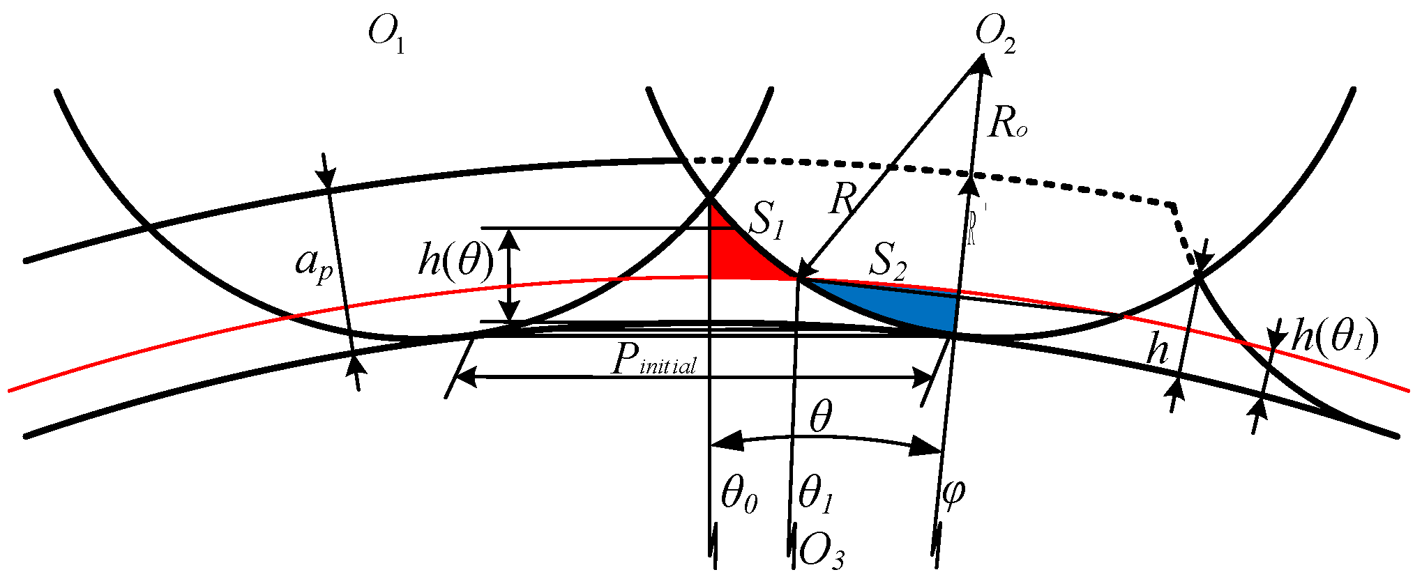
3. Surface Roughness Modeling Based on Residual Height
3.1. Surface Roughness without Wear
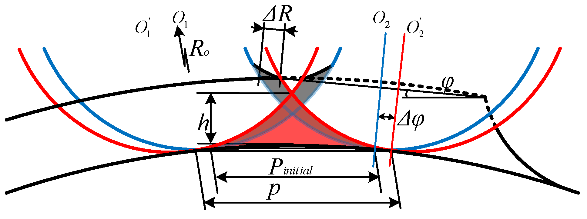
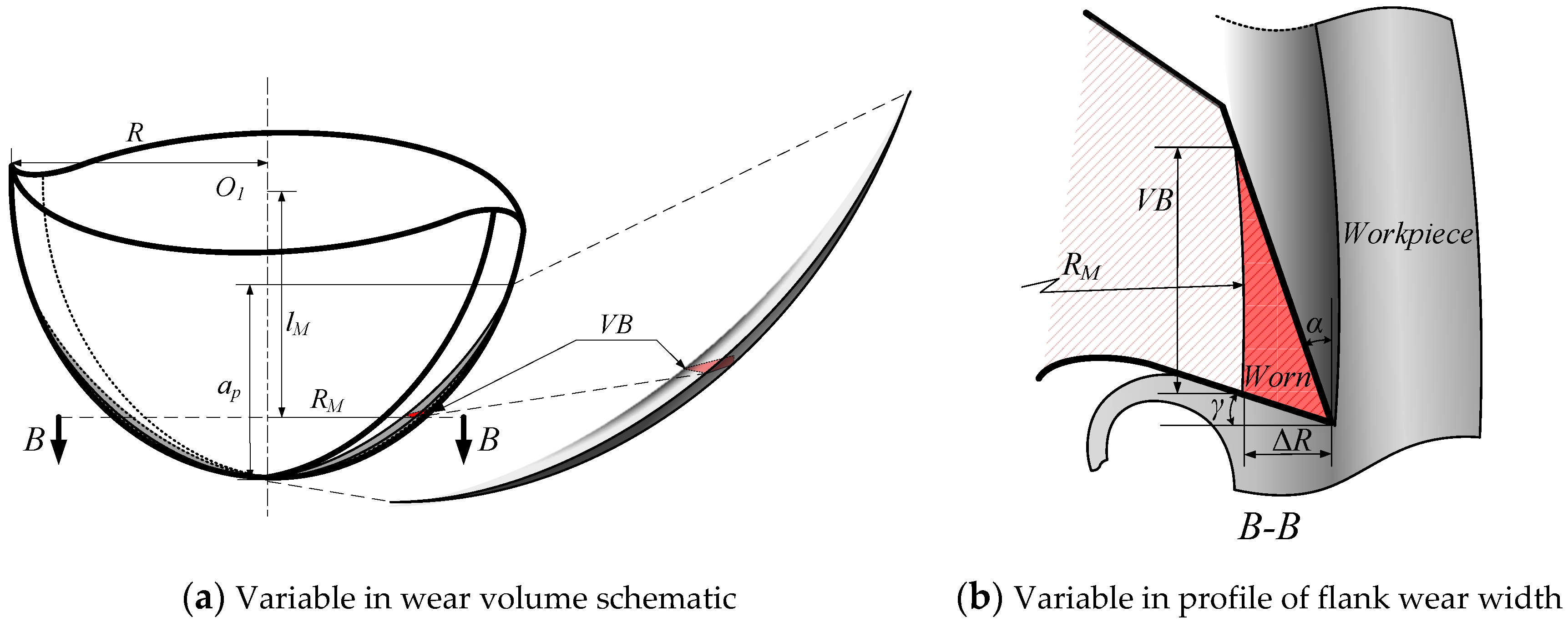
3.2. Surface Roughness under Flank Wear Condition
4. Experiment and Verification
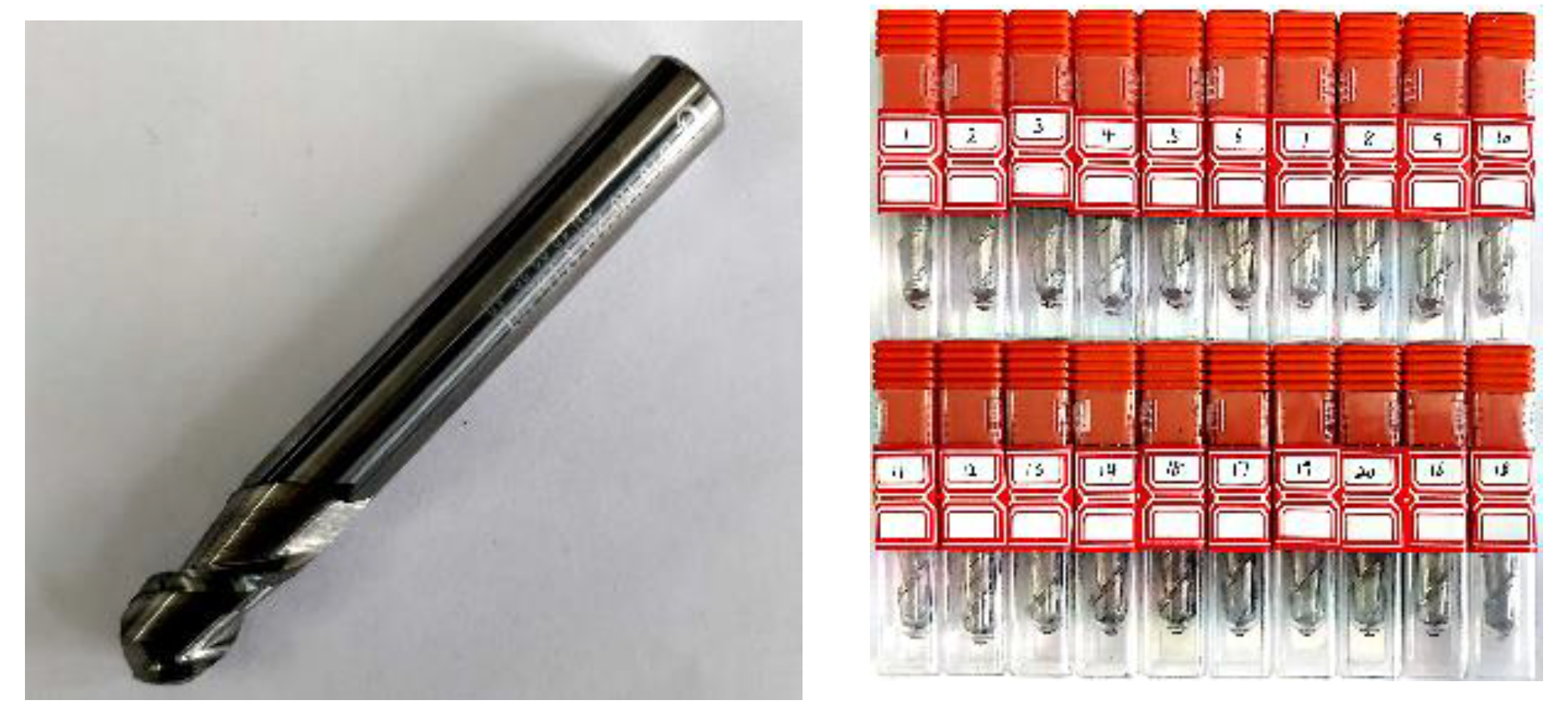
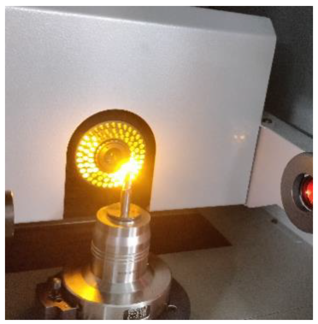
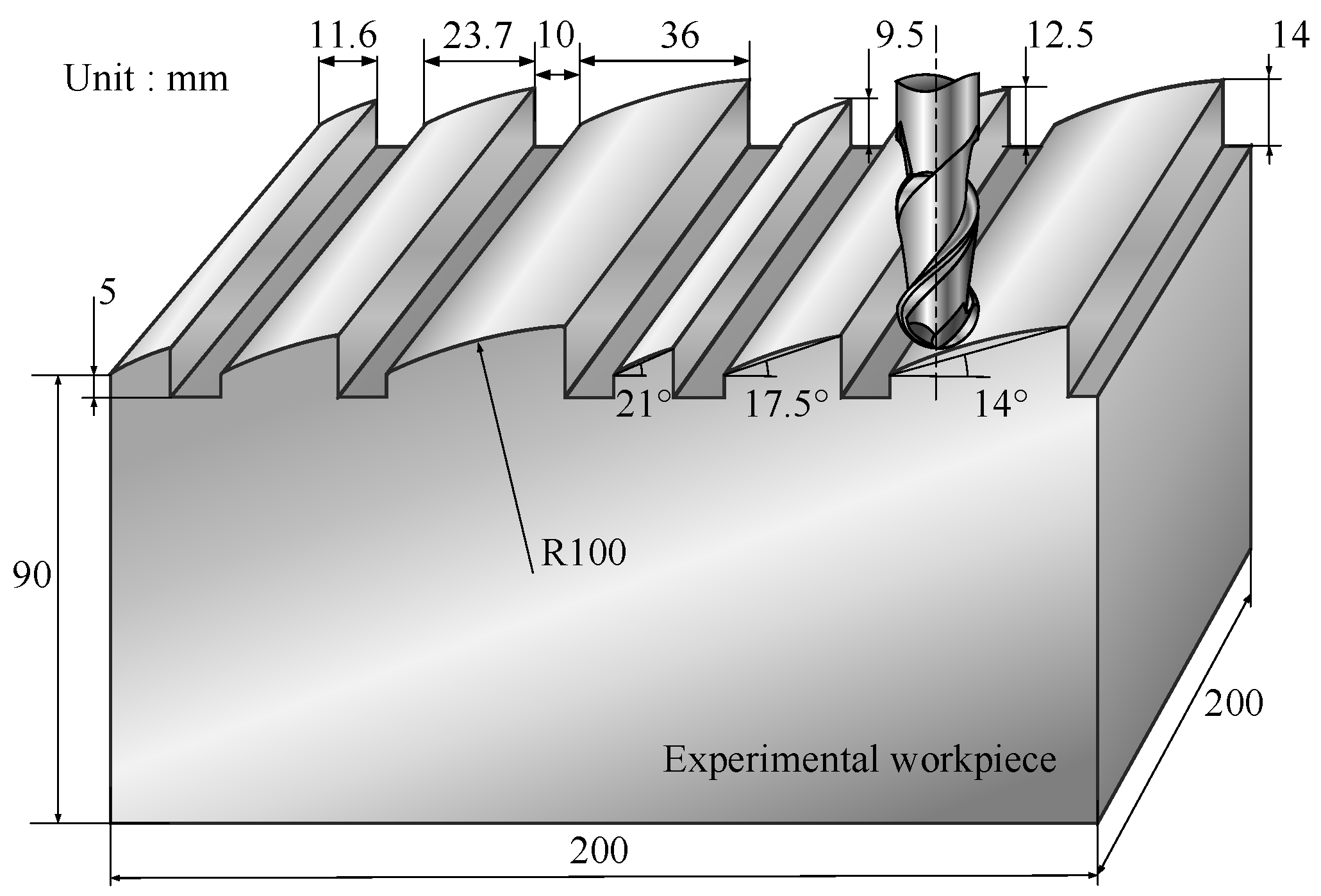
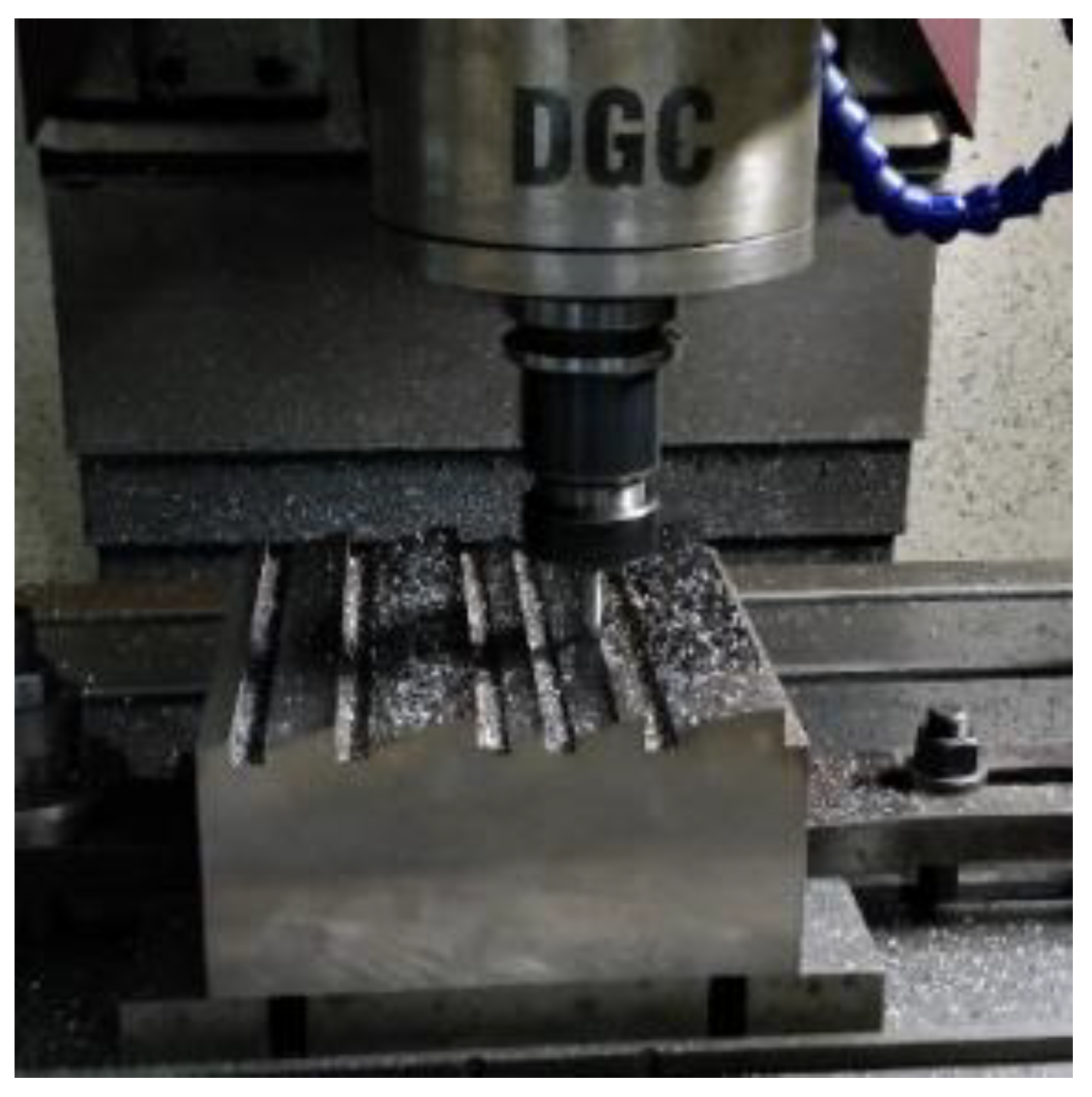
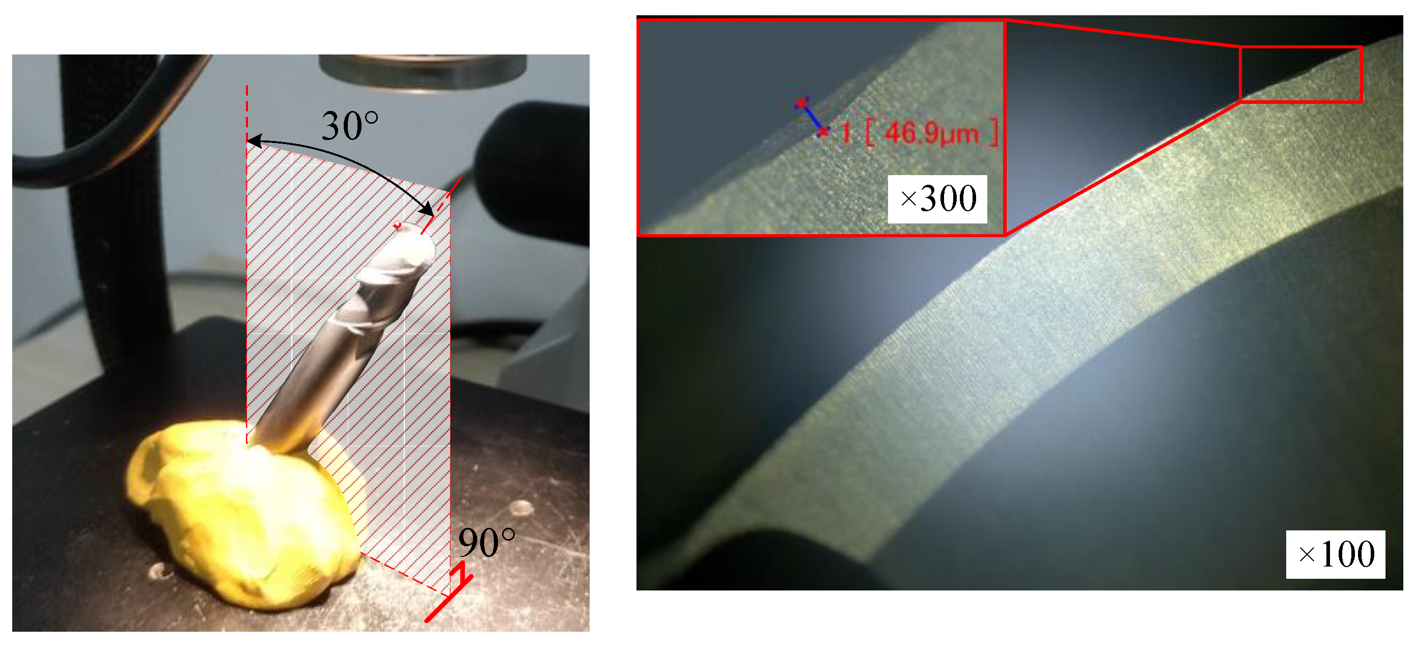
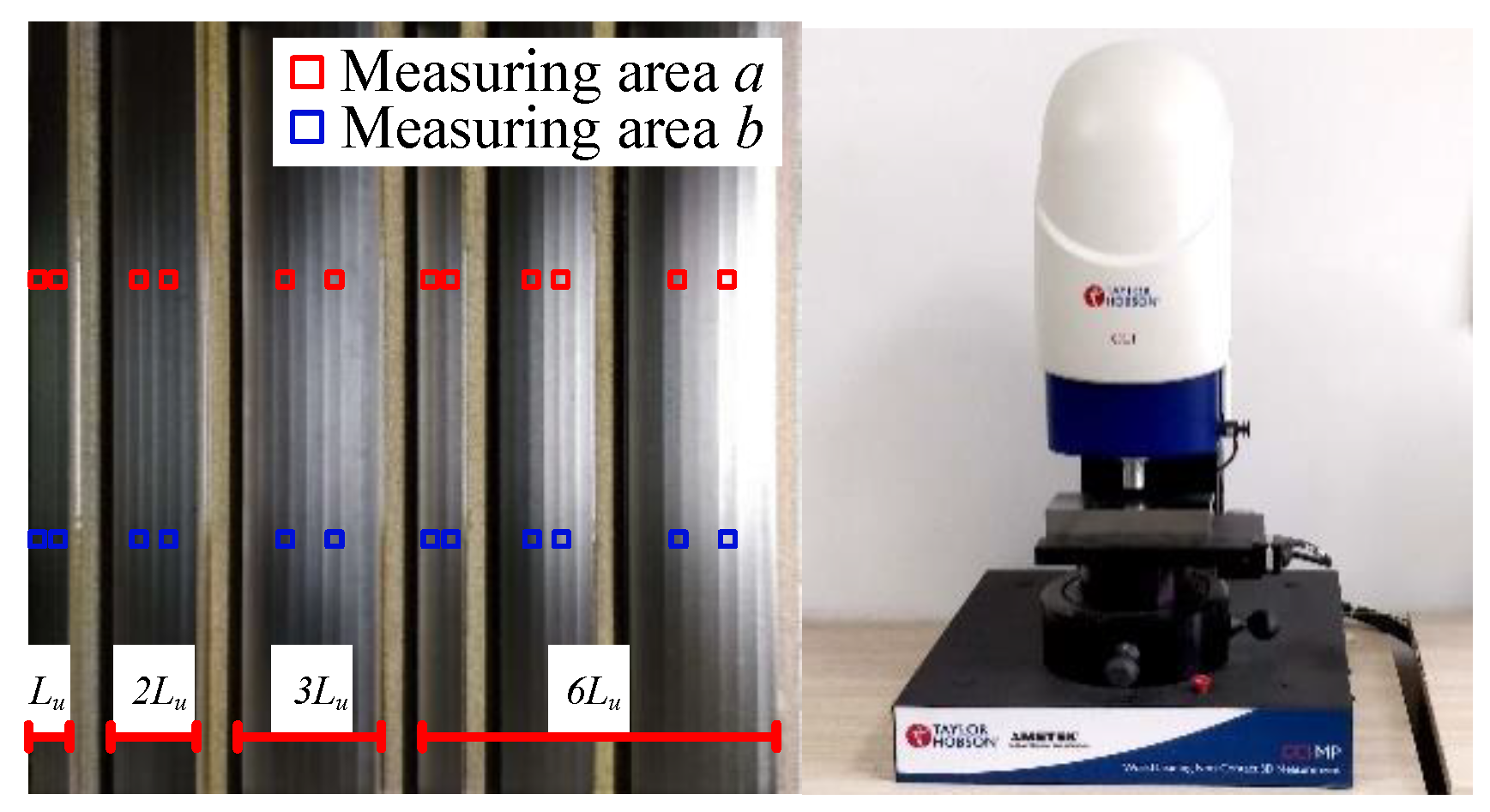
4.1. Experiment Preparation
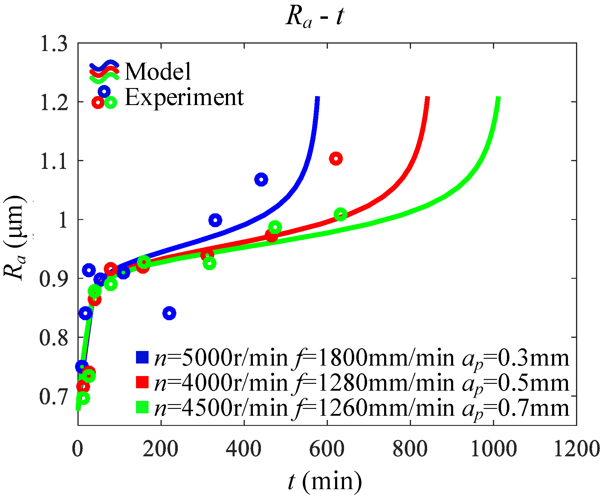
4.2. Model Verification
5. Model Simulation and Discussion
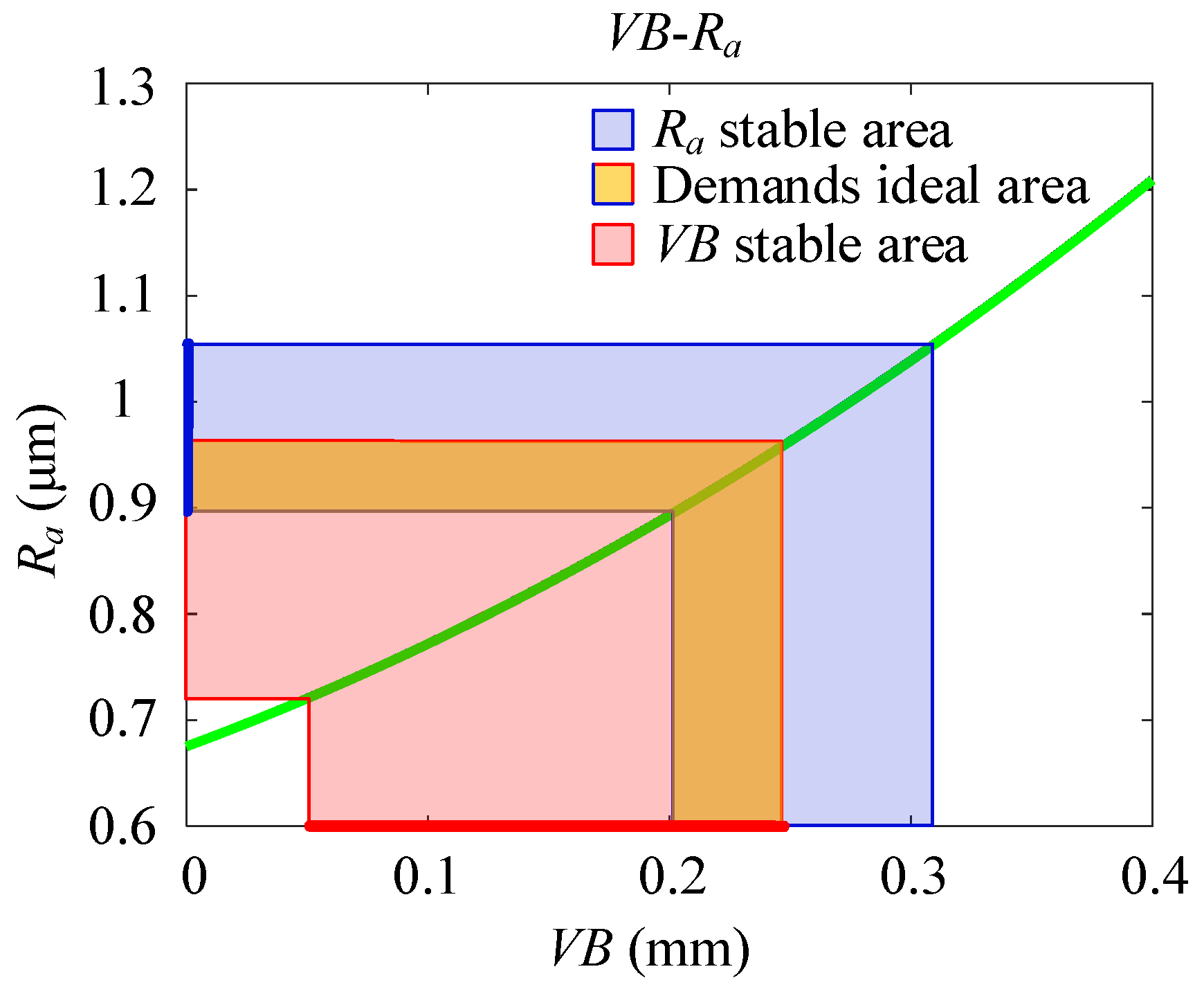
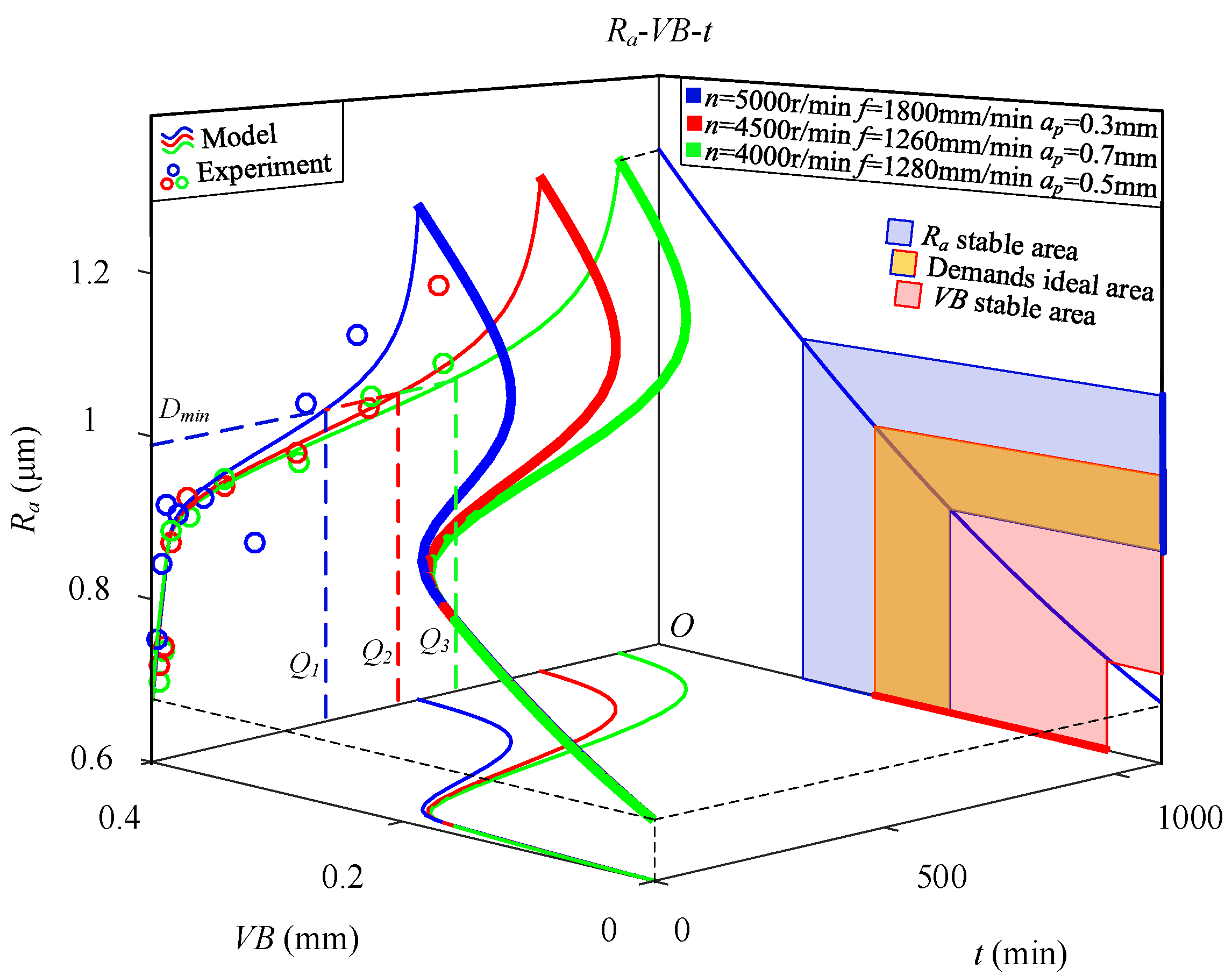
5.1. Derivation of Ra-VB Relationship
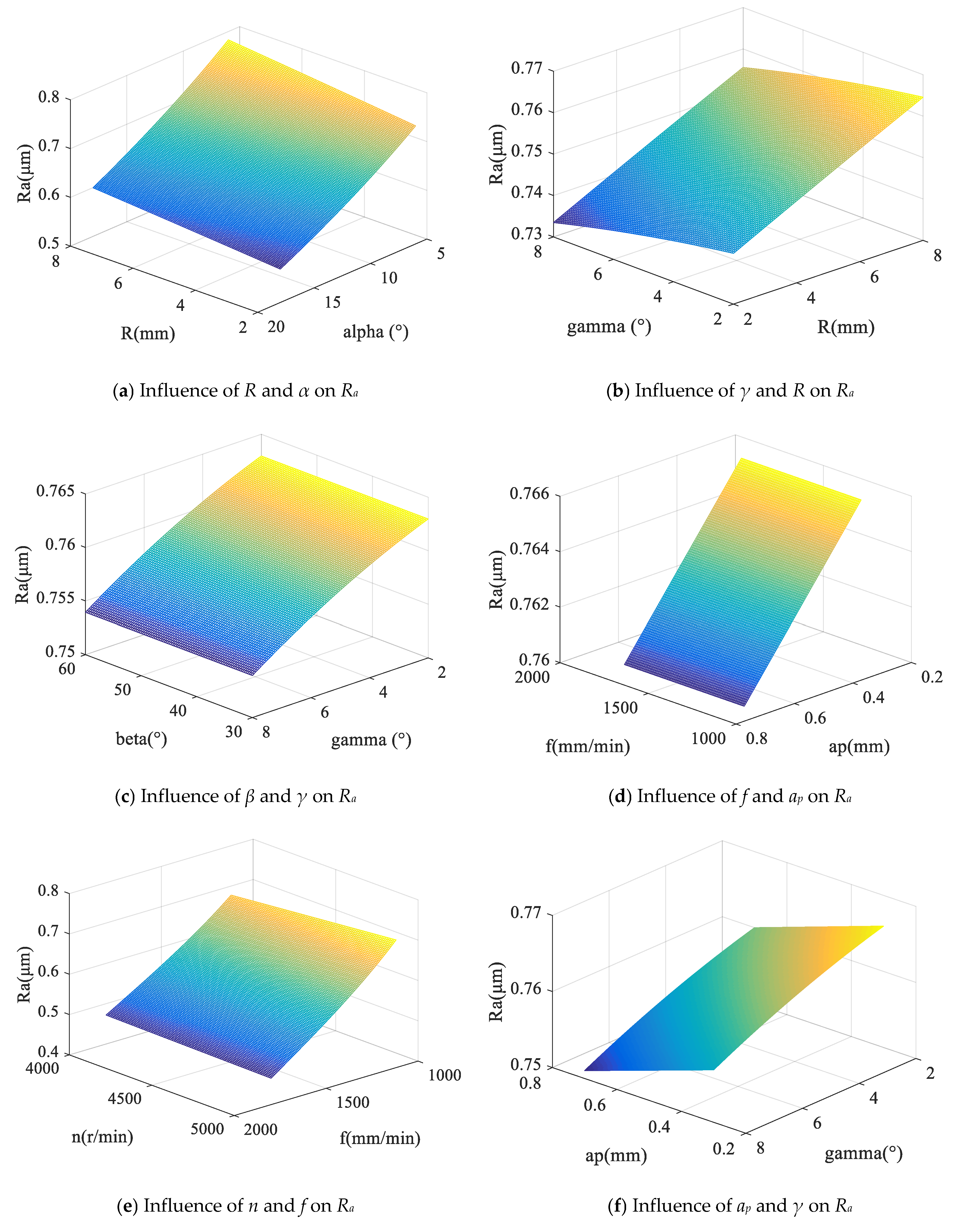
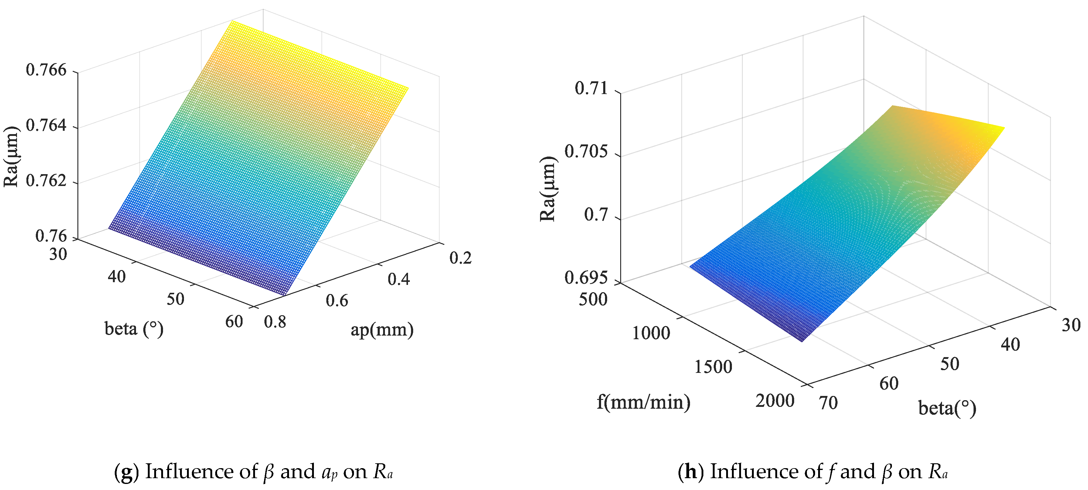
5.2. Analysis of Main Influencing Factors
6. General Method of Performance Design Based on the Analytical Model
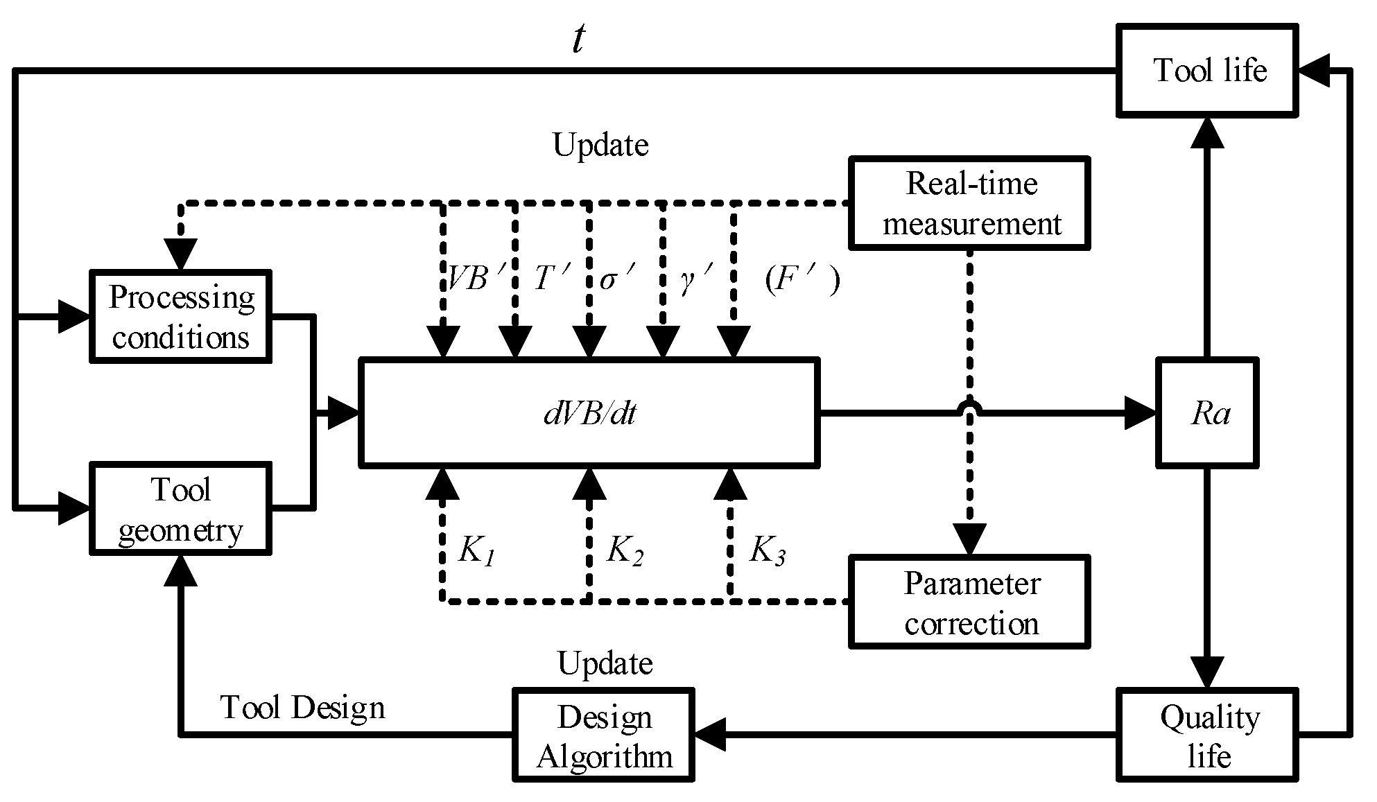
6.1. Theoretical Flowchart
6.2. Application and Development
7. Conclusions
- Among the many influencing factors, Ra, α, R, γ, ap, and β are relatively significant, compared with the other factors, the influence of f and n were not as significant in this study, however, this may be affected by their respective ranges of variation. These important factors should be prioritized in the design and use of a tool to ensure consistency of the processing quality.
- In many influential relationships, some factors either weaken or enhance the other, and the interaction characteristics of such factors should be utilized to balance the design during tool design or optimization.
- Attention should be paid to the simultaneous changes of a certain couple of factors during the tool design or optimization process as a higher change rate of Ra may occur.
- This research provides service performance quantification and a general method of cutting tool performance design. The method is shown to be feasible and can be used for tool performance design or optimization.
- The material property parameters of the surface roughness model and the time-varying wear model proved to change dynamically with the processing in the experiments.
- The model was established without considering crushing, built-up edge, and the slowing effect of the compound formed by the chemical reaction on the flank surface. Additionally, during the simulation process, the variation of the formula coefficients under different milling temperatures and time periods was not considered and the change of the tool geometry was not corrected with time. These are the main error sources of the model and simulation results.
Author Contributions
Funding
Conflicts of Interest
Abbreviations
| T | Tool life |
| Q | Quality life |
| t | Machining time |
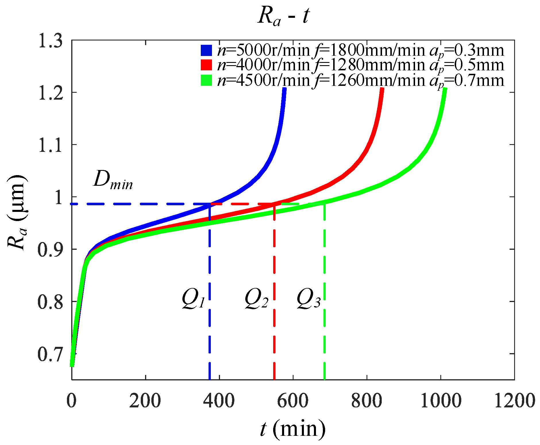
| Dmin | Minimum processing demand |
| Ra | Surface roughness |
| R | Ball radius |
| Z0 | Number of teeth |
| γ | Rake angle |
| α | Flank angle |
| β | Helix angle |
| n | Spindle speed |
| Vc | Milling speed |
| ap | Milling depth |
| aw | Milling width |
| f | Feed rate |
| fz | Feed per tooth |
| p | Line spacing |
| Pinitial | Initial line spacing value |
| ρ | Curvature (vertical to feed) |
| ρ’ | Curvature (along feed) |
| θ | Tool inclination angle |
| φ | Equivalent angle |
| ω | Final equivalent angle |
| Ro | Center distance |
| RM | Radius at maximum wear |
| lM | Depth at maximum wear |
| h | Residual height |
| l | Wear band length |
| T0 | Milling temperature |
| F | Milling force |
| σ | Average contact stress |
| ΔR | Radial wear |
| ΔV | Wear column |
| VB | Maximum flank wear |
| K1, K2, K3 | Comprehensive wear coefficient |
| K0, C0, | Model correction factor |
| a, b, c, d, g, e, n0 | Wear model parameters |
References
- Abele, E.; Hasenfratz, C.; Bucker, M. Modeling of process forces with respect to technology parameters and tool wear in milling Ti6Al4V. J. Prod. Eng. 2017, 11, 285–294. [Google Scholar] [CrossRef]
- Yue, C.; Gao, H.; Liu, X.; Liang, S.Y. Part functionality alterations induced by changes of surface integrity in metal milling process: A review. Appl. Sci. 2018, 8, 2550. [Google Scholar] [CrossRef]
- Ji, W.; Zhao, Z.; Liu, X. A GA-based optimization algorithm for cutting tool “shape-performance-application” integrated design approach. Proced. CIRP 2016, 56, 90–94. [Google Scholar] [CrossRef][Green Version]
- Ji, W.; Zhao, Z.; Liu, X. Tool shape-performance-application integrated design approach: A development and a numerical validation. Int. J. Adv. Manuf. Technol. 2017, 94, 1–7. [Google Scholar] [CrossRef]
- Liu, X.; Ji, W.; Fan, M.; Wang, C. Feature based cutting tool “shape-performance-application” integrating design approach. J. Mech. Eng. 2016, 52, 146–153. [Google Scholar] [CrossRef]
- Khan, M.R. Geometric modeling, design, and analysis of custom-engineered milling cutters. Jabalpur 2011, 2, 543–550. [Google Scholar]
- Huang, Y.; Liang, S.Y. Modeling of CBN tool flank wear progression in finish hard turning. J. Manuf. Sci. Eng. 2004, 126, 98–106. [Google Scholar] [CrossRef]
- Li, K.M.; Liang, S.Y. Flank wear model for near dry turning under built-up edge effect. Chin. J. Mech. Eng. 2012, 33, 123–132. [Google Scholar]
- Teitenberg, T.M.; Bayoumi, A.E.; Yucesan, G. Tool wear modeling through an analytic mechanistic model of milling processes. Wear 1992, 154, 287–304. [Google Scholar] [CrossRef]
- Bouzakis, K.D.; Paraskevopoulou, R.; Katirtzoglou, G. Predictive model of tool wear in milling with coated tools integrated into a CAM system. CIRP Ann. Manuf. Technol. 2013, 62, 71–74. [Google Scholar] [CrossRef]
- Zhao, Z.; Liu, X.; Yue, C. Time-varying analytical model of ball-end milling tool wear in surface milling. Int. J. Adv. Manuf. Technol. 2020, 1–15. [Google Scholar] [CrossRef]
- Biondani, G.B. Effect of cutting edge micro geometry on surface generation in ball end milling. CIRP Ann. 2019, 68, 571–574. [Google Scholar] [CrossRef]
- Kasim, M.S.; Hafiz, M.S.A. Investigation of surface topology in ball nose end milling process of Inconel 718. Wear Part. B 2019, 426-427, 1318–1326. [Google Scholar] [CrossRef]
- Ghoreishi, R.; Roohi, A.H.; Ghadikolaei, A.D. Evaluation of tool wear in high-speed face milling of Al/SiC metal matrix composites. J. Braz. Soc. Mech. Sci. Eng. 2019, 41, 146. [Google Scholar] [CrossRef]
- Cagrı, V.; Turgay, K.; Murat, S.; Senol, S. Evaluation of tool wear, surface roughness/topography and chip morphology when machining of Ni-based alloy 625 under MQL, cryogenic cooling and CryoMQL. J. Mater. Res. Technol. 2020, 9, 2079–2092. [Google Scholar]
- Reza, G.; Roohi, A.H.; Amir, D.G. Analysis of the influence of cutting parameters on surface roughness and cutting forces in high speed face milling of Al/SiC MMC. Mater. Res. Express 2018, 5, 56–73. [Google Scholar]
- Wojciechowski, S.; Twardowski, P. Tool life and process dynamics in high speed ball end milling of hardened steel. Proced. CIRP 2012, 1, 289–294. [Google Scholar] [CrossRef]
- Ahmad, F.; Gu, L.; Zhao, W.; Rajurkar, K.P. Tool path optimization based on wear prediction in electric arc sweep machining. J. Manuf. Processes 2020, 54, 328–336. [Google Scholar]
- De Aguiar, M.M.; Diniz, A.E.; Pederiva, R. Correlating surface roughness, tool wear and tool vibration in the milling process of hardened steel using long slender tools. Int. J. Mach. Tools Manuf. 2013, 68, 1–10. [Google Scholar] [CrossRef]
- Bouzakis, K.-D.; Aichouh, P.; Efstathiou, K. Determination of the chip geometry, cutting force and roughness in free form surfaces finishing milling, with ball end tools. Int. J. Mach. Tools Manuf. 2003, 43, 499–514. [Google Scholar] [CrossRef]
- Grzesik, W. Influence of tool wear on surface roughness in hard turning using differently shaped ceramic tools. Wear 2008, 265, 327–335. [Google Scholar] [CrossRef]
- Zhang, C.; Zhang, H.; Li, Y. Modelling and on-line simulation of surface topography considering tool wear in multi-axis milling process. Int. J. Adv. Manuf. Technol. 2015, 77, 735–749. [Google Scholar] [CrossRef]
- Tunc, L.T. Smart tool path generation for 5-axis ball-end milling of sculptured surfaces using process models. Robot. Comput. Integr. Manuf. 2019, 56, 212–221. [Google Scholar] [CrossRef]
- Wang, X.; Feng, C.X. Development of empirical models for surface roughness prediction in finish turning. Int. J. Adv. Manuf. Technol. 2002, 20, 348–356. [Google Scholar] [CrossRef]
- Mansour, A.; Abdalla, H. Surface roughness model for end milling: A semi-free cutting carbon casehardening steel (EN32) in dry condition. J. Mater. Process. Technol. 2002, 124, 183–191. [Google Scholar] [CrossRef]
- Lee, K.Y.; Kang, M.C.; Jeong, Y.H. Simulation of surface roughness and profile in high-speed end milling. J. Mater. Process. Technol. 2001, 113, 410–415. [Google Scholar] [CrossRef]
- Davim, J.P. Book review: Tribology of metal cutting by Viktor, P. Astakhov. Int. J. Mach. Mach. Mater. 2009, 5, 367–368. [Google Scholar] [CrossRef]
- Alauddin, M.; Baradie, M.A.E.; Hashmi, M.S.J. Prediction of tool life in end milling by response surface methodology. J. Mater. Process. Technol. 1997, 71, 456–465. [Google Scholar] [CrossRef]
- Sun, H.; Wang, Z.; Zhang, Y. Evaluation method of product—Service performance. Int. J. Comput. Integr. Manuf. 2012, 25, 150–157. [Google Scholar] [CrossRef]
- Urbikain, G.; de Lacalle, L.N.L. Modelling of surface roughness in inclined milling operations with circle-segment end mills. Simul. Model. Pract. Theory 2018, 84, 161–176. [Google Scholar] [CrossRef]
- Eshi, U. Cutting and Grinding Processing; Mechanical Industry Press: Beijing, China, 1982; pp. 34–36. [Google Scholar]
- Kan, N. Advances in stochastic theory of fatigue damage accumulation. Adv. Mech. Eng. 1999, 31, 43–65. [Google Scholar]
- Su, Y.; He, N.; Li, L. An experimental investigation of effects of cooling/lubrication conditions on tool wear in high-speed end milling of Ti-6Al-4V. Wear 2006, 261, 760–766. [Google Scholar] [CrossRef]
- Ezugwu, E.O.; Wang, Z.M. Titanium alloys and their machinability—A review. J. Mater. Proc. Technol. 1997, 68, 262–274. [Google Scholar] [CrossRef]
- Sui, S.C.; Feng, P.F.; Mou, W.P. Temperature modeling analysis for milling of titanium alloy. Key Eng. Mater. 2016, 693, 928–935. [Google Scholar] [CrossRef]
- Werner, J.; Andreas, K. Soil surface roughness measurement—Methods, applicability, and surface representation. Catena 2005, 64, 174–192. [Google Scholar]
- Yue, C.; Gao, H.; Liu, X.; Ling, S.Y.; Wang, L. A review of chatter vibration research in milling. Chin. J. Aeronaut. 2019, 32, 1–28. [Google Scholar] [CrossRef]
- Wojciechowski, S.; Mrozek, K. Mechanical and technological aspects of micro ball end milling with various tool inclinations. Int. J. Mech. Sci. 2017, 134, 424–435. [Google Scholar] [CrossRef]


| N | 20 |
|---|---|
| Kendall’s W identification coefficient | 0.961 |
| Asymptotic significance | 0 < 0.05 |
| G | Tool Code | n (r/min) | ap (mm) | fz (mm) | L (mm) |
|---|---|---|---|---|---|
| 3 | 5 | 5000 | 0.3 | 0.18 | 3 Lu |
| 4 | 5 | 5000 | 0.3 | 0.18 | 6 Lu |
| 5 | 5 | 5000 | 0.3 | 0.18 | 12 Lu |
| 6 | 5 | 5000 | 0.3 | 0.18 | 24 Lu |
| 6a | 5 | 5000 | 0.3 | 0.18 | 36 Lu |
| 6b | 5 | 5000 | 0.3 | 0.18 | 48 Lu |
| 7 | 7 | 4000 | 0.5 | 0.16 | 3 Lu |
| 8 | 7 | 4000 | 0.5 | 0.16 | 6 Lu |
| 9 | 7 | 4000 | 0.5 | 0.16 | 12 Lu |
| 10 | 7 | 4000 | 0.5 | 0.16 | 24 Lu |
| 10a | 7 | 4000 | 0.5 | 0.16 | 36 Lu |
| 10b | 7 | 4000 | 0.5 | 0.16 | 48 Lu |
| 14 | 12 | 4500 | 0.7 | 0.14 | 3 Lu |
| 15 | 12 | 4500 | 0.7 | 0.14 | 6 Lu |
| 16 | 12 | 4500 | 0.7 | 0.14 | 12 Lu |
| 17 | 12 | 4500 | 0.7 | 0.14 | 24 Lu |
| 17a | 12 | 4500 | 0.7 | 0.14 | 36 Lu |
| 17b | 12 | 4500 | 0.7 | 0.14 | 48 Lu |
| N | 2 |
|---|---|
| Kendall’s W identification coefficient | 0.897 |
| Asymptotic significance | 0.011 < 0.05 |
| TGP | T&WP | CWC | WEC | REC |
|---|---|---|---|---|
| γ = 5° | a = 15255 | K1 = 9.838 × 10⁻¹⁰ | K = 40,923 | K0 = 2000 |
| α = 12° | b = 1.6 | K2 = 6.647 × 10⁻¹⁰ | C = 18.13 | C0 = 0.53 |
| β = 50° | e = 23,054 | K3 = 2.923 × 10⁻⁶ | ||
| R = 5 mm | g = 3.62 × 10⁻⁴ |
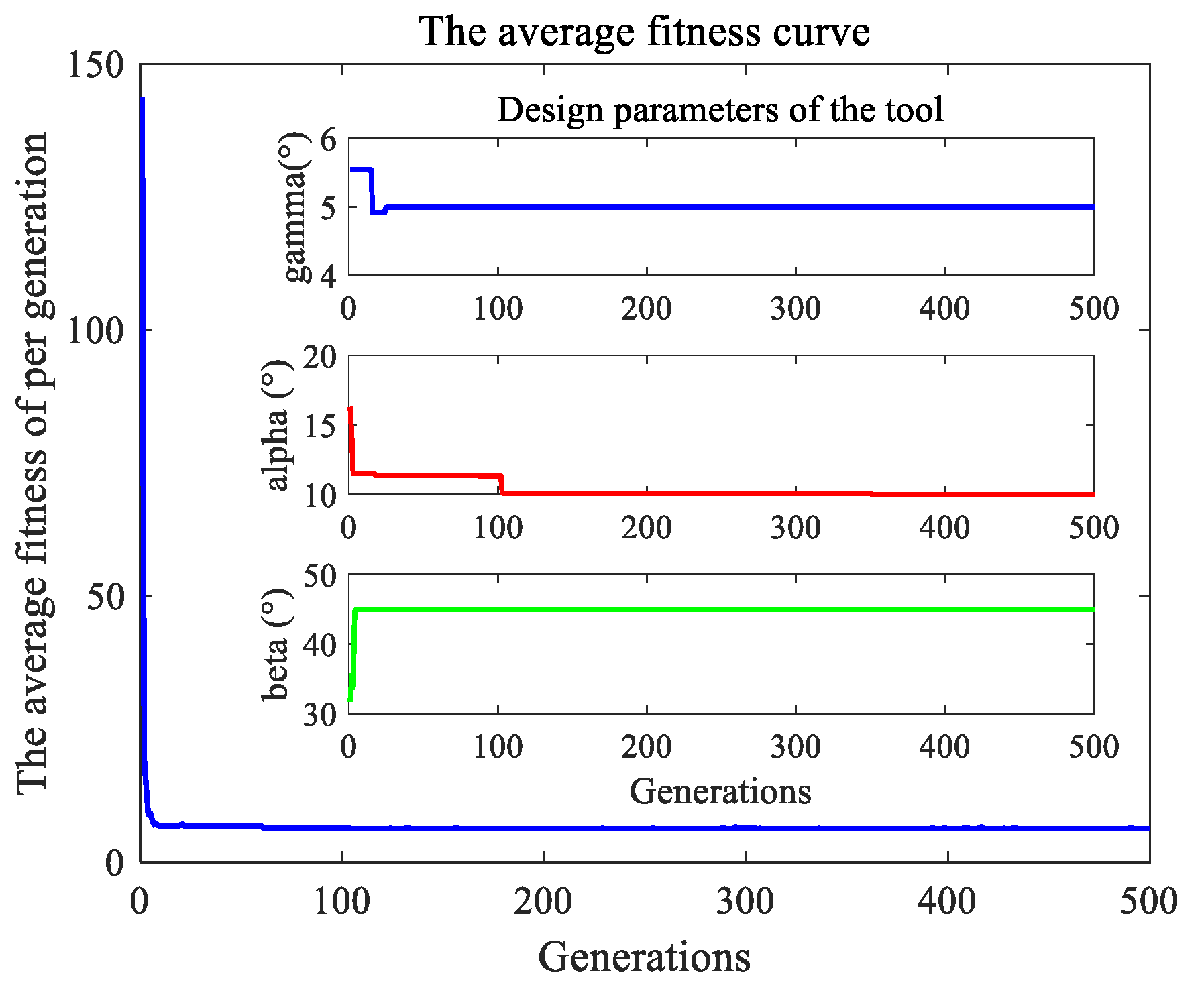
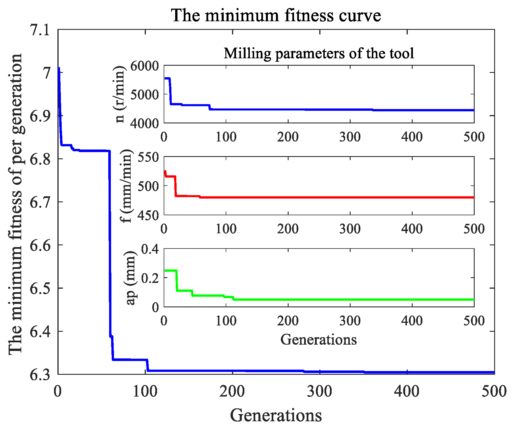
| Tool Design Parameters | Tool Milling Parameters | ||
|---|---|---|---|
| γ (°) | 5 | n (r/min) | 4083.6 |
| α (°) | 10 | f (mm/min) | 482.2 |
| β (°) | 45.8 | ap (mm) | 0.064 |
© 2020 by the authors. Licensee MDPI, Basel, Switzerland. This article is an open access article distributed under the terms and conditions of the Creative Commons Attribution (CC BY) license (http://creativecommons.org/licenses/by/4.0/).
Share and Cite
Zhao, Z.; Liu, X.; Yue, C.; Li, R.; Zhang, H.; Liang, S. Tool Quality Life during Ball End Milling of Titanium Alloy Based on Tool Wear and Surface Roughness Models. Appl. Sci. 2020, 10, 3316. https://doi.org/10.3390/app10093316
Zhao Z, Liu X, Yue C, Li R, Zhang H, Liang S. Tool Quality Life during Ball End Milling of Titanium Alloy Based on Tool Wear and Surface Roughness Models. Applied Sciences. 2020; 10(9):3316. https://doi.org/10.3390/app10093316
Chicago/Turabian StyleZhao, Zemin, Xianli Liu, Caixu Yue, Rongyi Li, Hongyan Zhang, and Steven Liang. 2020. "Tool Quality Life during Ball End Milling of Titanium Alloy Based on Tool Wear and Surface Roughness Models" Applied Sciences 10, no. 9: 3316. https://doi.org/10.3390/app10093316
APA StyleZhao, Z., Liu, X., Yue, C., Li, R., Zhang, H., & Liang, S. (2020). Tool Quality Life during Ball End Milling of Titanium Alloy Based on Tool Wear and Surface Roughness Models. Applied Sciences, 10(9), 3316. https://doi.org/10.3390/app10093316